Deep Learning-Based Classification of Weld Surface Defects

Abstract

In order to realize the non-destructive intelligent identification of weld surface defects, an intelligent recognition method based on deep learning is proposed, which is mainly formed by convolutional neural network (CNN) and forest random. First, the high-level features are automatically learned through the CNN. Random forest is trained with extracted high-level features to predict the classification results. Secondly, the weld surface defects images are collected and preprocessed by image enhancement and threshold segmentation. A database of weld surface defects is established using pre-processed images. Finally, comparative experiments are performed on the weld surface defects database. The results show that the accuracy of the method combined with CNN and random forest can reach 0.9875, and it also demonstrates the method is effective and practical.

1. Introduction

As a traditional processing method, the welding process is widely used in aerospace, machine design, energy generation, shipbuilding, petrochemical engineering, and other industries. Welding is a complicated process, which is often affected by the welding process and environmental uncertainties, and it is easy to produce welding defects such as overlap, pore, spatter, slag inclusion, and incomplete fusion. Therefore, it is necessary to conduct research on the detection and identification of weld surface defects. Common non-destructive testing methods for welds include ultrasonic testing [1], ray detection [2], and eddy current testing [3]. However, these methods have some limitations: (1) ray detection can easily result in side-effects on the human body; (2) ultrasonic testing is susceptible to the location, orientation, and shape of the defect; (3) eddy current testing is only applicable to conductive metal materials or non-metallic materials that can induce eddy currents.

During the last decade, computer vision became an important field of artificial intelligence, which has been widely used in weld defect detection. It generally includes four steps: image acquisition, image preprocessing, feature extraction, and classification [4]. Feature extraction is one of the most critical technologies. Many studies have been carried out on feature extraction and classification of weld defects. Sun et al. [5] isolated the defect features of thin-walled workpiece based on the background subtraction of Gaussian mixture model and constructed a decision tree to discern weld defects. Valavanis et al. [6] extracted texture and geometric features of different weld defects and used support vector machine (SVM), k-nearest neighbor (KNN), and artificial neural network (ANN) to complete the classification. Yin et al. [7] proposed a new method to automatically extract four geometric features from Lissajous figures and use machine learning-based classifiers to identify defects. Boaretto et al. [8] obtained defect features by the exposure technique of double wall double image (DWDI) and used multi-layer perception (MLP) to continuously classify defect or no-defect. Zapata et al. [9] selected the shape and direction of weld defects as classification features, and proposed an adaptive network based fuzzy inference system to detect welding defects. Zahran et al. [10] extracted feature from the power density spectra (PDS) of the weld segmented areas and used ANN to match features in order to recognize different defects. In References [11,12], a method based on principal component analysis (PCA) and SVM was proposed. It can effectively transform weld defects images to principal component space through PCA and complete the classification using SVM. However, the above feature extraction and classification methods only utilize the texture or geometric features of the weld defects images, and it is not ideal to form suitable features for classification.

The history of deep learning originates from neuroscience experiments. As early as 1943, neurologist McCulloch and mathematician Pitts constructed the first artificial neuron model according to the structure and working principle of biological neurons, which was called the “MCP model”. Since then, many researchers have proposed various neural network models. However, due to the problem of gradient disappearance in the training method proposed at that time, it has been difficult to use this powerful model. This problem was not solved until the emergence of deep learning methods [13] in 2006. Krizhevshy et al. [14] used AlexNet to make a breakthrough in ImageNet image classification competition, deep learning showed unprecedented development prospects. After that, researchers have proposed ZFNet, VGGNet, GoogLeNet, and ResNet models for large-scale image classification. Compared with the traditional feature extraction methods, these methods do not need to implement any features of the pre-selected image. It can learn the high-level features of the target from the sample data by supervised learning [15].

Recently, deep learning methods have been widely applied in weld defects detection. Yang et al. [16] proposed a modified convolutional neural network (CNN) to implement classification in X-ray weld images. Hou et al. [17] construct a deep convolutional neural network (DCNN) to extracted high-level features from X-ray images. Khumaidi et al. [18] introduced the idea of Gaussian kernel into deep learning. The purpose is to ensure that the main information of the image is extracted while minimizing the occurrence of noise and interference and improving the classification accuracy. In Reference [19], Liu Bin et al. utilized the VGG16 based fully CNN to inspect welding defect images using the idea of transfer learning. High precision classification is achieved with a relatively small data set. In Reference [20], Hou et al. proposed a deep neural network based on sparse automatic encoder. It learns the feature information of the image in an unsupervised way, and then uses the softmax classifier with supervised learning to identify the defects such as pore and undercut. In Reference [21], Du et al. adopted feature pyramid network (FPN) and RoIAlign to realize defect detection of X-ray images of automobile aluminum casting parts. The above methods usually need to construct deep CNN architecture and utilize softmax to handle classification tasks. However, in the case of fewer training samples, there is a poor performance for softmax that the features are confusing.

In order to solve the problems mentioned, an intelligent recognition method based on deep learning is proposed. What is more, random forest is selected as the final classification algorithm because random forest has good fault-tolerant ability and low generalization errors on the issue of dealing with classification. The overview of the proposed method is shown in Figure 1. It is mainly formed by two modules: CNN and forest random. The CNN architecture is constructed to automatically extract high-level features of weld surface defects images. Random forest is trained by using the high-level features to accomplish the classification task. In addition, the welding surface defects images including normal, overlap, spatter, and pore are preprocessed by image enhancement and threshold segmentation. A database of weld surface defects is established using pre-processed images and is taken as input data. Finally, comparative experiments are carried out to verify the effective and practical of proposed method.

The structure of this paper is organized as follows. The Section 2 gives specific architecture of the CNN module. In Section 3, the classification module applying random forests is described in detail. Weld defect image pre-processing and experimentation are given in Section 4. The Section 5 summarizes the article.

2. CNN-Based Feature Extraction

2.1. Background

The basic idea of deep learning is to construct a deep nonlinear network structure. It initializes the weights through unsupervised pre-training methods, and then fine-tunes through supervised training. The problem of gradient disappearance is effectively suppressed with ReLU activation function. Deep learning can gradually transform the initial low-level feature into high-level features through multi-layer processing, which is beneficial to complete complex tasks such as image [22], speech [23], and language [24].

At present, typical deep learning architectures include CNN [25,26], deep belief networks (DBNs) [27], sparse automatic coding (SAEs) [28], and deep Boltzmann machines (RBMs) [29]. In view of the excellent feature extraction performance of convolution neural network in image classification [25,26] and object detection [30,31], CNN is applied to automatically extract high-level features of weld surface defects images in Section 2.2.

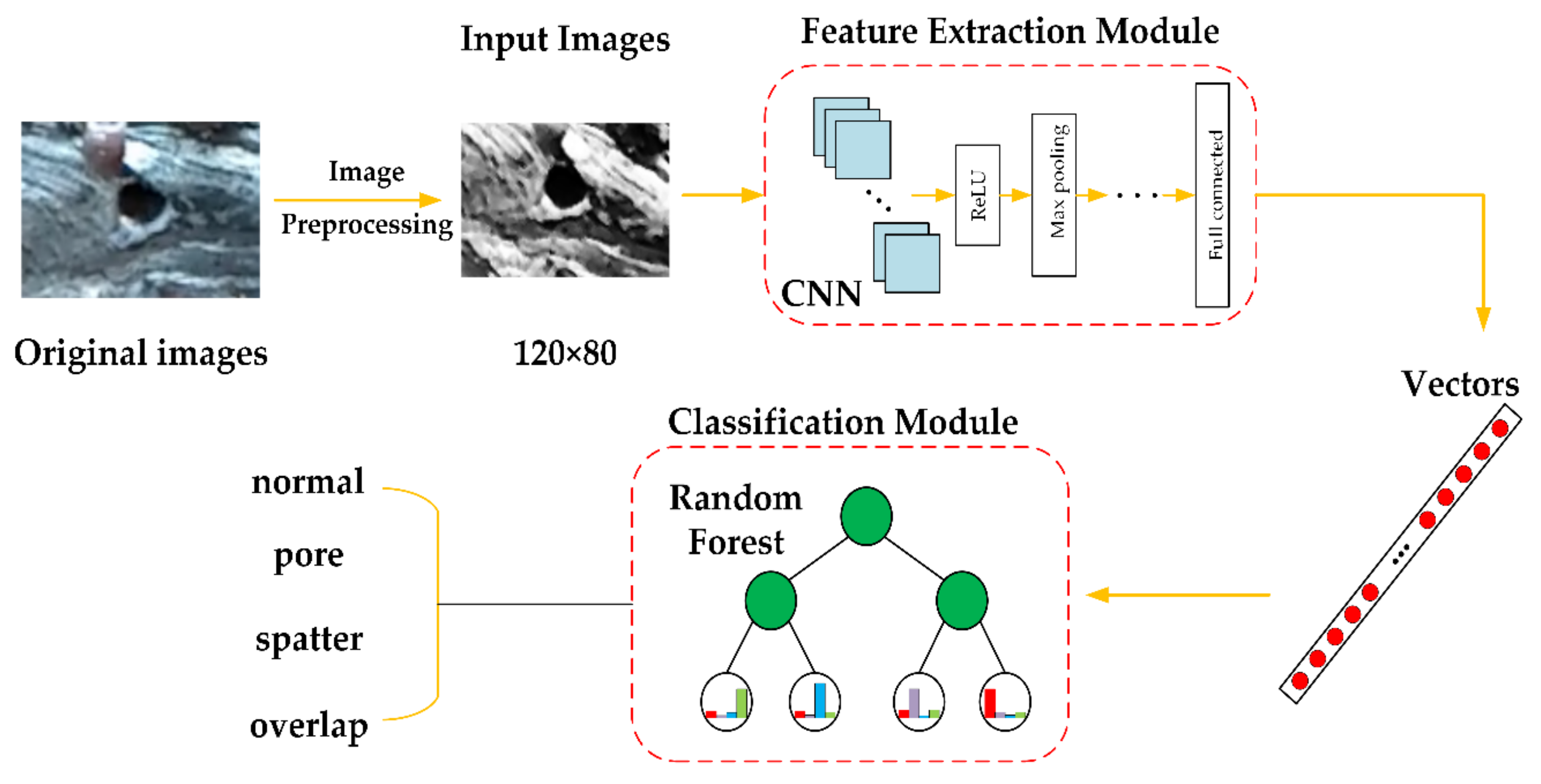
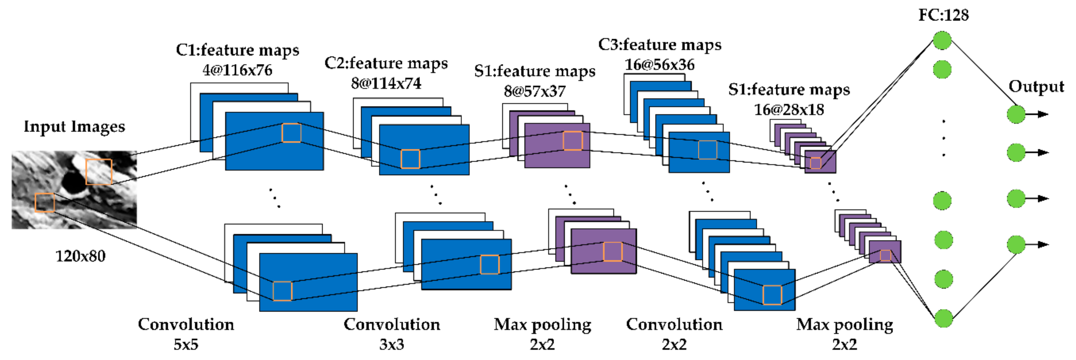
2.2. Feature Extraction Module

The task of CNN is to automatically extract high-level features of the weld surface defects images. Inspired by LeNet-5 [32], a deep CNN architecture is constructed by overlaying multiple convolutional layers. A typical convolutional layer usually contains convolution, nonlinear function activation and pooling operations. Figure 2 shows the specific architecture of the CNN. The CNN mainly is made up of three convolutional layers, two pooling layers, one fully connected layer, and one softmax layer. The input of the CNN contains training and validation images with 80 × 120 (height × width).

In our paper, the convolutional layers are named C1, C2, and C3, respectively, which consists of 4, 8, 16 filters. The size of corresponding filters is 5 × 5, 3 × 3, and 2 × 2. Let $x^l$ denotes the out of convolutional layers, and it can be expressed as:

$$x^l=f(b^l+{\displaystyle \sum _j^J{\displaystyle \sum _i^I{w}_{i,j}^l{x}_{i,j}^{l-1}}})$$

(1)

$$f\left(x\right)=ReLU\left(x\right)=\left\{\begin{array}{ll}x& x>0\\ 0& x\le 0\end{array}\right.$$

(2)

where $\left(J,I\right)$ denotes the size of the filters, $J$ is the height of the filters, and $I$ is the width of the filters. $b^l$ denotes the bias of the convolutional layer. $x^{l-1}$ denotes the output of the previous convolutional layer. $w^l$ denotes the weight of convolutional layer. $f\left(\cdot \right)$ is the nonlinear activation function. ReLU activation function is selected and is shown as Equation (2).

Pooling operation [33] is another important component. The pooling layers are named S1 and S2. Two max-pooling layers with stride 2 are used to combine a 2 × 2 patch of the convolutional layers C2 and C3. Each pooling layer corresponds to the previous convolutional layer. The neurons in the pooling layer perform aggregation statistics on specific regions in the convolution layer to achieve the purpose of down-sampling for the input feature map. Common pooling operations include average pooling, maximum pooling, and random pooling. The maximum pooling used in this paper is expressed as follows:

$$a_j=\underset{N\times N}{max}\left(a_i^{N\times N}u\left(n,n\right)\right)$$

(3)

where $u\left(n,n\right)$ is the window function, which is applied to calculate the maximum value of $a_j$ in the neighborhood.

After a series of convolution, activation, and pooling, the fully connected layer splices the feature that is extracted from convolutional layer C3 and max-pooling layer S2 into a 128-dimensional vector. The output of the fully connected layer can be obtained by:

$$v^m=f\left(w^m{x}^{m-1}+b^m\right)$$

(4)

where $b^m$ denotes the bias of the fully connected layer. $w^m$ denotes the weights of the fully connected layer. $x^{m-1}$ denotes the output of the previous max-pooling layer. $f\left(\cdot \right)$ is the ReLU activation function. The CNN is trained by the cross-entropy function. The details explain of CNN are given in

Table 1. The details of CNN architecture.

Layer	C1	C2	S1	C3	S2
Details	4 filters 5 × 5, ReLU, stride 1 × 1	8 filters 3 × 3, ReLU, stride 1 × 1	max pooling, stride 2 × 2	16 filters 2 × 2, ReLU, stride 1 × 1	max pooling, stride 2 × 2

.

3. Classification with Random Forest

3.1. Random Forest Algorithm

Random forest [34] is a machine learning algorithm proposed by Leo breiman in 2001. It is an integrated algorithm based on decision tree. The main idea is to use multiple weak classifiers to form a strong classifier by voting. For the classification task, the random forest algorithm mainly includes three steps: bootstrap sampling, constructing decision tree, and voting.

The bootstrap sampling refers to a uniform sampling method with a return. Self-sampling is useful when the data set is small. It can generate different training sets from the initial data set, which is beneficial to improve the image recognition ability. Decision tree construction is usually one of three methods: iterative dichotomiser 3 (ID3), C4.5, classification and regression tree (CART). This paper uses the CART algorithm to generate decision trees. CART assumes that the decision tree is a binary tree, and the internal node features are divided into left and right branches according to the threshold. Generally, the feature with the smallest Gini index in the subset and its corresponding threshold are selected as the optimal feature and the optimal segmentation point. The data set is allocated to the left branch node and the right branch node. The feature tree with the smallest Gini index splits the binary tree to form a classification tree to form a random forest. The Gini index of feature M is defined as follows:

$$Gini\left(D_j,M\right)=\frac{\left|D_j^1\right|}{\left|D_j\right|}Gini\left(D_j^1\right)+\frac{\left|D_j^2\right|}{\left|D_j\right|}Gini\left(D_j^2\right)$$

(5)

where $Gini\left(D_j\right)=1-{\displaystyle \sum _{i=1}^N{\left(p_i\right)}^2}$, $D_j$ denotes to the $j\mathrm{th}$ training set of the sample, and p_i denotes the proportion of the $i\mathrm{th}$ sample in the training set.

Based on the results of each classification tree, a voting mechanism is used to determine the final classification result. The classification function is expressed as follows:

$$H\left(x\right)=\mathrm{a}\mathrm{r}\mathrm{g}\mathrm{m}\mathrm{a}\mathrm{x}{\displaystyle \sum _{i=1}I\left(h_i\left(x\right)\right)}$$

(6)

where $I\left(\cdot \right)$ denotes the indicative function, ranging from 0 to 1. $H\left(x\right)$ denotes the combined classification model. $h_i$ denotes the single decision tree classification model.

3.2. Classification Module

Training random forests with 128-dimensional vectors to achieve classification results. The primary task of the random forest algorithm is to create decision trees. A decision tree consists of a terminal node, several internal nodes, and several leaf nodes. First, $T$ sample sets $D_l$ ($l=1,2,3,...,T$) that every sample set contains $m$ training samples are sampled by using the bootstrap from deep feature vector $v^m$, and will be used as the terminal root of the decision tree. Terminal nodes are designed to ensure that the training sample sets for each decision tree are different. Secondly, in order to avoid over-fitting of the classification results, it is necessary to randomly choose features in the process of establishing internal nodes in a single decision tree. $f$ features are elected from $h$ features without replacement. The rule for feature selection is generally followed as $f=\sqrt{h}$, here ($f\le h$). Next, the feature attribute with the smallest Gini index in the feature subset $\left\{f\right\}$ is calculated based on Equation (5). The attribute and the corresponding threshold are taken as the optimal partition attribute and the optimal split point at the non-special node. The decision tree stops splitting until the Gini index of the feature in the sample set is less than a predetermined threshold. Repeat the above steps until $T$ decision trees are generated.

Another task of the random forest is to perform predictions using the created random forest. The classification model consisting of $T$ decision trees uses the voting method based on Equation (6) to calculate the largest number of votes among decision trees, and the decision tree with the largest number of votes is selected the final classification result.

In a nutshell, the classification process with random forest is summarized in Algorithm 1 in details.

Algorithm 1 Random Forest for Classification

1: Input: 2: Initialization 3: procedure Random Forest 4: For $t$ = 1 to $T$ do 5: Draw n bootstrap sample $D_l$ from input data 6: Build a decision tree $T$ on $D_l$ by recursively repeating the following steps for each terminal root 7: Select $f$ features without replacement from the $h$ features 8: Calculate the smallest Gini index of feature attribute among the feature subset $\left\{f\right\}$ based on Equation (5) 9: end procedure 10: Output: the ensemble of trees ${\left\{T\right\}}_1^T$ 11: Classification: 12: $H\left(x\right)=\arg \max {\displaystyle \sum _{i=1}I\left(h_i\left(x\right)\right)}$

4. Experimental Results.

4.1. Settings and Experimental Environment

In our experiment, the welding equipment used to produce welds images includes ABB-IRB2600industrial robot, Kemppi-SYN welding machines, kemppi-DT400 wire feeder and welding torch. The welding parameters are set as follows: wire feed rate is 4 m/min, welding speed is 50 cm/min, weld shield gas is CO₂, gas flow rate is 20 L/min, the adjustment range of the arc voltage is 16–25 V. All weld images are produced with same equipment and constant parameters. 400 weld surface defects images are collected which include normal, overlap, spatter and pore four categories. Each type of property contained 100 weld defects with different appearances and different postures with a resolution of 120 × 80. Image preprocessing is given in Section 4.2. A database is established using pre-processed weld surface defects images.

In order to verify the effectiveness and practicality of the proposed method for the weld surface defects identification, a comparison experiment with other methods is carried out, which is given in Section 4.3 and Section 4.4. The experimental environment is a 64-bit Windows 10 system with i5 CPU, 8 GB memory, and 2.30 GHz basic frequency. The software programming environment is python. The implementation is based on the framework in Keras, and the backend of Keras are TensorFlow and Theano. The weld surface defects images used for model training were randomly selected for each category of 80 images, and the remaining 80 were used for model validation.

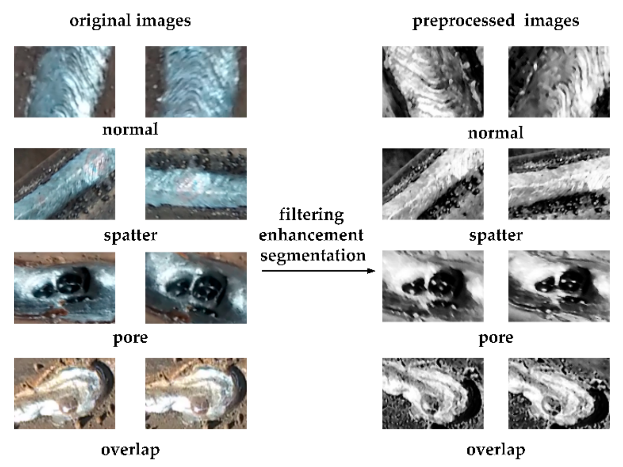
4.2. Image Preprocessing

The actual welding process is often affected by a complex welding environment, weld parameters, and human factors. The acquired images of weld surface defects usually contain a mass of redundant information. In order to effectively extract the weld defect feature information for the CNN, the images need to be pre-processed.

Figure 3 shows partially examples of pre-processed results for weld surface defects images. All weld surface defects images that are collected in Section 4.1 are preprocessed through filtering, enhancement, and segmentation. First, the median filter is used to dispose the collected images of weld surface to eliminate the noise of the original images. Secondly, in order to enhance the gradation value of the weld area, the images are enhanced by gradation processing. Next, the OTSU algorithm is chosen to isolate the weld defect area from the other elements in the original images, which segmented an appropriate area of the weld surface defects to facilitate subsequent feature extraction.

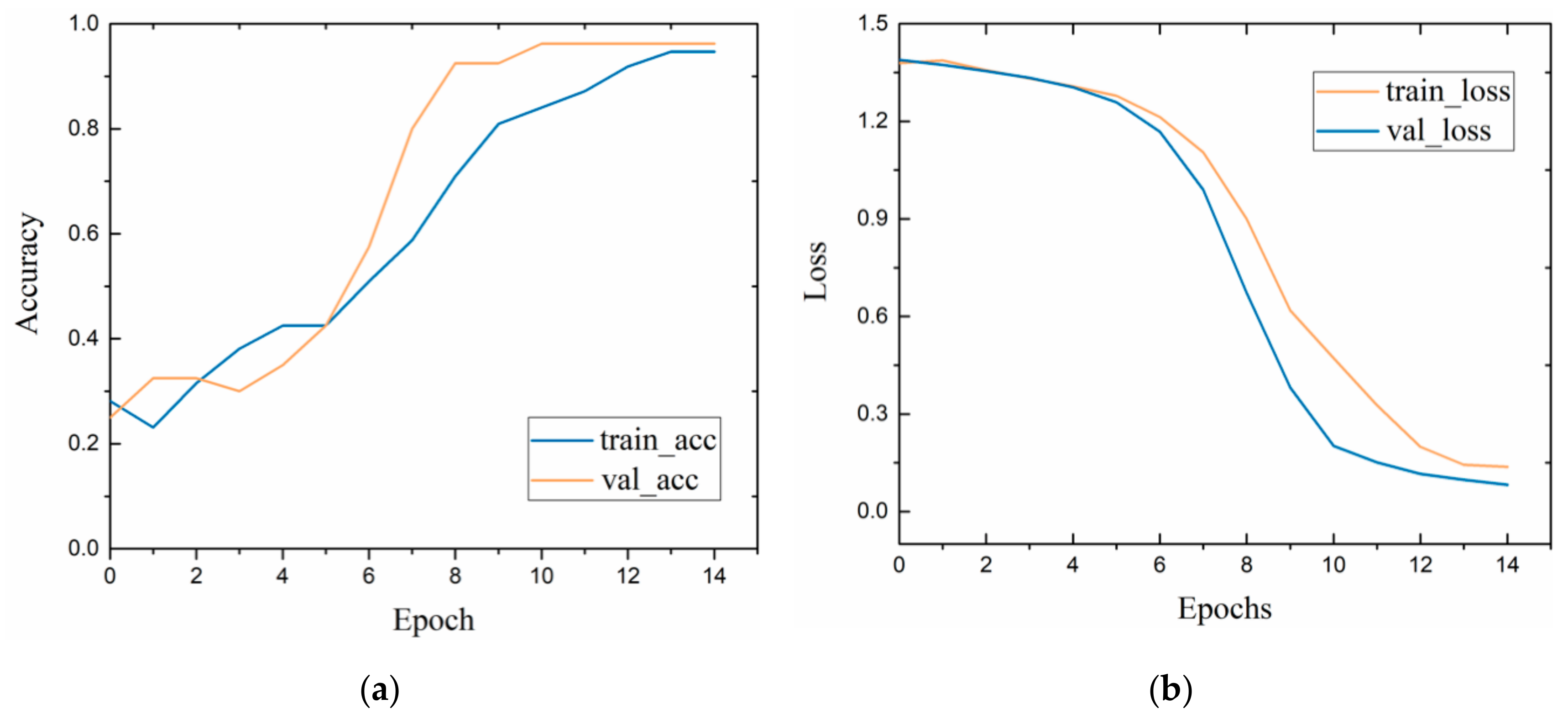
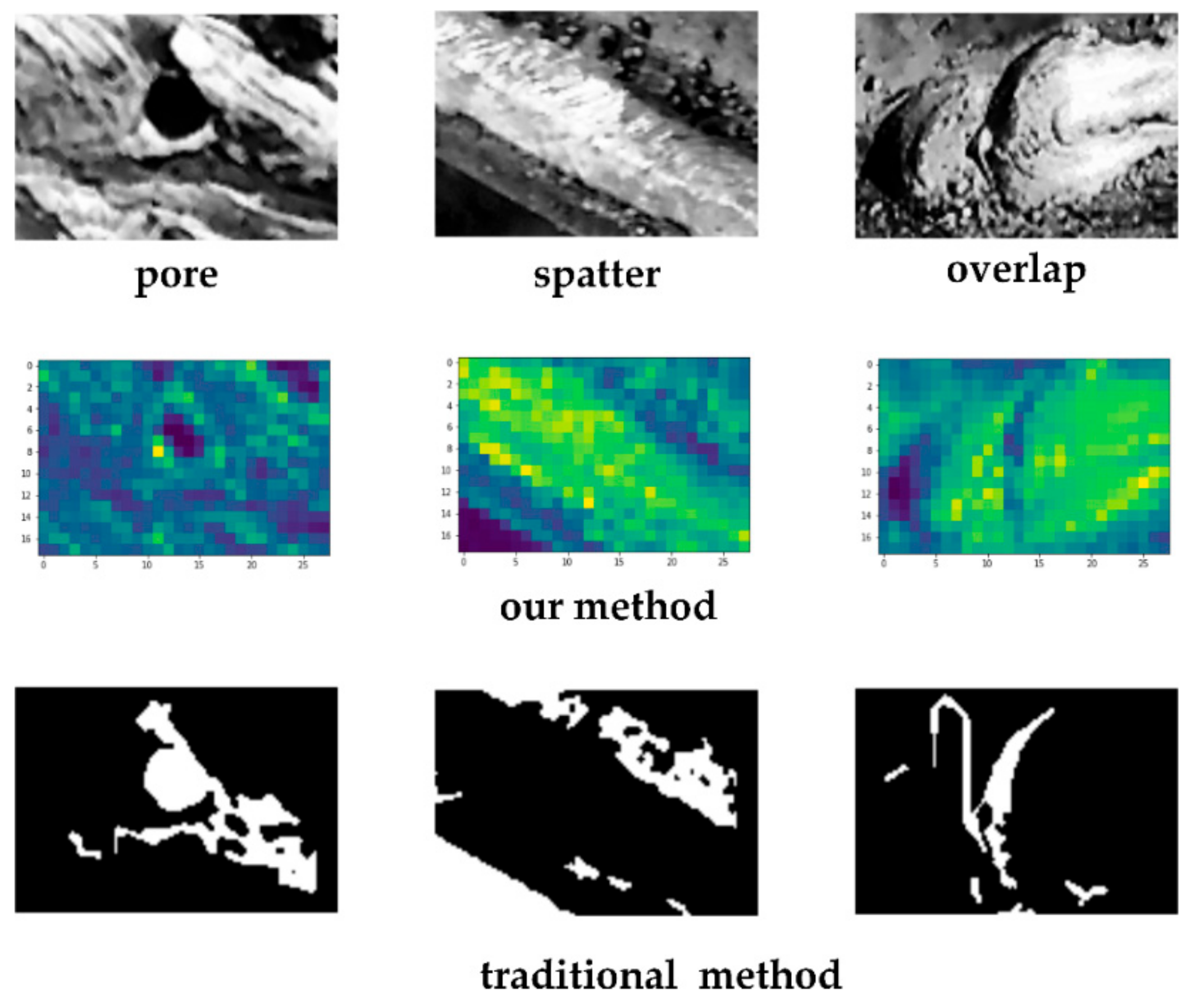
4.3. Evaluation of Feature Extraction Module

In the feature extraction module, stochastic gradient descent (SGD) is selected as optimizer of the CNN. The learning rate is set as an adaptive value, which it trains the model with a predetermined value (0.001) and decays with a constant value 1 × 10⁻⁸. The value of momentum is 0.9. The CNN is trained using the pre-processed weld surface defects database. The training process is shown in Figure 4. Figure 4a shows the trend for accuracy of the training and validation accuracy as the number of iterations increases. After fifteen epochs, the CNN can achieve a maximum training accuracy of 94.69. Figure 4b gives the trend for the objective function loss value of the training and validation as the number of iterations increases. The loss value of objective function gradually becomes smoother to prove that the CNN is convergent.

In Reference [6], texture and geometrical features need to be artificially described. In References [11,12], all images need to be vectorized in advance, and the covariance matrix dimension after the vector is too large, which affects the feature extraction speed. In our feature extraction module, the CNN automatically learns high-level features from the images. In order to evaluate the effectiveness of our feature extraction module, we compared the feature extraction method in our paper with traditional image process methods. As is given in Figure 5, our method extracted the high-level features, which can better represent the semantic information of the image and facilitate the classification algorithm to identify. However, the texture or geometric features segmented by the traditional method are not obvious enough, which can cause feature confusion and affect the accuracy of classification. Furthermore, the feature extraction module in our paper can avoid supererogatory human consumption and simplify process.

4.4. Comparison to Other Methods

In order to evaluate the effectiveness of the classification module, a comparative experiment is carried out. In this section, two machine learning-based classifiers are applied to compare with our classification module for defects recognition and they are SVM and softmax. The high-level features that are extracted in Section 2.2 are used as training data. Then, the train random forest, SVM and softmax are trained with the input of extracted high-level features. The classification accuracy results in terms of the high-level features can be obtained as follows and are listed in

Table 2. Accuracy results of different classification methods.

Method	Accuracy
CNN + Random Forest	0.9875
CNN + SVM	0.95
CNN + Softmax	0.9469

.

It can be seen from Table 2 that the accuracy of the method combined with CNN and random forest can reach 0.9875. Moreover, it shows a better performance than other classifiers. It indicates that the random forest has better generalization ability and robustness. Simultaneously, it also can demonstrate the method is effective and practical. In addition, the SVM and softmax classifiers show high classification accuracies, which can reach to 0.95 and 0.9469, respectively. It can testify that the CNN for feature extraction is effective.

5. Conclusions

This paper proposes a method based on deep learning to identify weld defects. The high-level feature of the weld surface defects images are extracted by the CNN, which fully exploits the ability of the CNN to extract image features and simplifies the feature extraction process. The classification identification is realized by random forest classification algorithm with stronger generalization ability and robustness. Experiments were carried out based on the weld surface defects database. The results show that the maximum accuracy of the proposed method is 0.9875, which can meet the requirements of classification of weld surface defects in actual production. The effectiveness and practicability of the proposed method are verified.

The image feature extraction and recognition process of weld surface defects achieved in this paper are all carried out offline, which is difficult to meet the real-time application in actual industrial production. Secondly, there are intermittent steps in the method proposed in this paper, which affects the recognition efficiency to some extent. Therefore, defect identification and optimized integration of algorithms for real-time extracted weld surface images will be the focus of the next phase.

References

1. Petcher, P.A.; Dixon, S. Weld defect detection using PPM EMAT generated shear horizontal ultrasound. NDT E Int. 2015, 74, 58–65. [Google Scholar] [CrossRef] [Green Version]
2. Zou, Y.R.; Du, D.; Chang, B.H.; Ji, L.H.; Pan, J.L. Automatic weld defect detection method based on Kalman filtering for real-time radiographic inspection of spiral pipe. NDT E Int. 2015, 72, 1–9. [Google Scholar] [CrossRef]
3. Dziczkowski, L. Elimination of coil liftoff from eddy current measurements of conductivity. IEEE Trans. Instrum. Meas. 2013, 62, 3301–3307. [Google Scholar] [CrossRef]
4. Mery, D.; Arteta, C. Automatic defect recognition in x-ray testing using computer vision. In Proceedings of the IEEE Winter Conference on Applications of Computer Vision, Santa Rosa, CA, USA, 24–31 March 2017. [Google Scholar]
5. Sun, J.; Li, C.; Wu, X.J.; Palade, V.; Fang, W. An effective method of weld defect detection and classification based on machine vision. IEEE Trans. Ind. Inform. 2019. [Google Scholar] [CrossRef]
6. Valavanis, I.; Kosmopoulos, D. Multiclass defect detection and classification in weld radiographic images using geometric and texture features. Expert Syst. Appl. 2010, 37, 7606–7614. [Google Scholar] [CrossRef]
7. Yin, Z.Y.; Ye, B.; Zhang, Z.L. A novel feature extraction method of eddy current testing for defect detection based on machine learning. NDT E Int. 2019. [Google Scholar] [CrossRef]
8. Boaretto, N.; Centeno, T.M. Automated detection of welding defects in pipelines from radiographic images DWDI. NDT E Int. 2017, 86, 7–13. [Google Scholar] [CrossRef]
9. Zapata, J.; Vilar, R.; Ramón, R. Performance evaluation of an automatic inspection system of weld defects in radiographic images based on neuro-classifiers. Expert Syst. Appl. 2011, 38, 8812–8824. [Google Scholar] [CrossRef]
10. Zahran, O.; Kasban, H.; El-Kordy, M.; El-Samie, F.E.A. Automatic weld defect identification from radiographic images. NDT E Int. 2013, 57, 26–35. [Google Scholar] [CrossRef]
11. Jiang, H.Q.; Zhao, Y.L.; Gao, J.M.; Zhao, W. Weld defect classification based on texture features and principal component analysis. Insight Destruct. Test. Cond. Monit. 2016, 58, 194–200. [Google Scholar] [CrossRef]
12. Mu, W.L.; Gao, J.M.; Jiang, H.Q.; Zhao, W. Automatic classification approach to weld defects based on PCA and SVM. Insight Destruct. Test. Cond. Monit. 2013, 55, 535–539. [Google Scholar] [CrossRef]
13. Hinton, G.E.; Salakhutdinov, R.R. Reducing the dimensionality of data with neural networks. Science 2006, 313, 504–507. [Google Scholar] [CrossRef] [PubMed]
14. Krizhevsky, A.; Sutskever, I.; Hinton, G.E. ImageNet classification with deep convolutional neural networks. Adv. Neural Inform. Proc. Syst. 2012, 25, 1097–1105. [Google Scholar] [CrossRef]
15. Lecun, Y.; Bengio, Y.; Hinton, G.E. Deep learning. Nature 2015, 521, 436–444. [Google Scholar] [CrossRef]
16. Yang, N.N.; Niu, H.J.; Chen, L.; Mi, G.H. X-ray weld image classification using improved Convolutional Neural Network. AIP Conf. Proc. 2018, 1995. [Google Scholar] [CrossRef]
17. Hou, W.H.; Ye, W.; Yi, J.; Zhu, C.A. Deep features based on a DCNN model for classifying imbalanced weld flaw types. Measurement 2019, 131, 482–489. [Google Scholar] [CrossRef]
18. Khumaidi, A.; Yuniarno, E.M.; Purnomo, M.H. Welding defect classification based on convolution neural network (CNN) and Gaussian kernel. In Proceedings of the International Seminar on Intelligent Technology and Its Applications, Surabaya, Indonesia, 28–29 August 2017; pp. 261–265. [Google Scholar]
19. Liu, B.; Zhang, X.Y.; Gao, Z.Y.; Chen, L. Weld defect images classification with VGG16-Based neural network. In Proceedings of the International Forum on Digital TV and Wireless Multimedia Communications, Shanghai, China, 8–9 November 2017; pp. 215–223. [Google Scholar]
20. Hou, W.H.; Wei, Y.; Guo, J.; Jin, Y.; Zhu, C.A. Automatic detection of welding defects using deep neural network. J. Phys. Conf. Ser. 2018, 933, 012006. [Google Scholar] [CrossRef]
21. Du, W.Z.; Shen, H.Y.; Fu, J.Z.; Zhang, G.; He, Q. Approaches for improvement of the X-ray image defect detection of automobile casting aluminum parts based on deep learning. NDT E Int. 2019, 107. [Google Scholar] [CrossRef]
22. Wang, L.Z.; Zhang, J.B.; Liu, P.; Choo, K.K.R.; Huang, F. Spectral–spatial multi-feature-based deep learning for hyperspectral remote sensing image classification. Soft Comput. 2017, 21, 213–221. [Google Scholar] [CrossRef]
23. Noda, K.; Yamaguchi, Y.; Nakadai, K.; Okuno, H.G.; Ogata, T. Audio-visual speech recognition using deep learning. Appl. Intell. 2015, 42, 722–737. [Google Scholar] [CrossRef]
24. Hirschberg, J.; Manning, C.D. Advances in natural language processing. Science 2015, 349, 261–266. [Google Scholar] [CrossRef] [PubMed]
25. Simonyan, K.; Zisserman, A. Very deep convolutional networks for large-scale image recognition. In Proceedings of the IEEE Conference on Computer Vision and Pattern Recognition, Columbus, OH, USA, 24–27 June 2014. [Google Scholar]
26. Szegedy, C.; Liu, W.; Jia, Y.Q.; Sermanet, P.; Reed, S.; Anguelov, D.; Erhan, D.; Vanhoucke, V.; Rabinovich, A. Going deeper with convolutions. In Proceedings of the IEEE Conference on Computer Vision and Pattern Recognition, Columbus, OH, USA, 24–27 June 2014. [Google Scholar]
27. Hinton, G.E.; Osindero, S.; The, Y. A fast learning algorithm for deep belief nets. Neural Comput. 2006, 18, 1527–1554. [Google Scholar] [CrossRef] [PubMed]
28. Wang, F.; Lee, N.; Sun, J.M.; Hu, J.Y.; Ebadollahi, S. Automatic group sparse coding. In Proceedings of the AAAI Conference on Artificial Intelligence, San Francisco, CA, USA, 7–11 August 2011. [Google Scholar]
29. Roux, N.L.; Bengio, Y. Representational power of restricted Boltzmann machines and deep belief networks. Neural Comput. 2008, 20, 1631–1649. [Google Scholar] [CrossRef] [PubMed]
30. Cai, Z.W.; Fan, Q.F.; Feris, R.S.; Vasconcelos, N. A unified multi-scale deep convolutional neural network for fast object detection. In Proceedings of the European Conference on Computer Vision, Amsterdam, The Netherlands, 8–16 October 2016; pp. 354–370. [Google Scholar]
31. Lin, T.Y.; Dollar, P.; Girshick, R.; He, K.M.; Hariharan, B.; Belongie, S. Feature pyramid networks for object detection. In Proceedings of the IEEE Conference on Computer Vision and Pattern Recognition, Honolulu, HI, USA, 21–26 July 2017; pp. 2117–2125. [Google Scholar]
32. Lecun, Y.L.; Bottou, L.; Bengio, Y.; Haffner, P. Gradient-based learning applied to document recognition. Proc. IEEE 1998, 86, 2278–2324. [Google Scholar] [CrossRef] [Green Version]
33. Scherer, D.; Müller, A.; Behnke, S. Evaluation of pooling operations in convolutional architectures for object recognition. In Proceedings of the International Conference on Artificial Neural Networks, Thessaloniki, Greece, 15–18 September 2010; pp. 92–101. [Google Scholar]
34. Breiman, L. Random Forest. Mach. Learn. 2001, 45, 5–32. [Google Scholar] [CrossRef]
Figure 1. The overview of proposed method.
Applsci 09 03312 g001
Figure 2. The architecture of convolutional neural network (CNN).
Applsci 09 03312 g002
Figure 3. Partial examples of pre-processed results for weld surface defects images including normal, overlap, spatter, and pore. All weld surface defects images have a resolution of 120 × 80.
Applsci 09 03312 g003
Figure 4. (a) The accuracy of the training and validation. (b) The objective function loss value of the training and validation.
Applsci 09 03312 g004
Figure 5. Comparison of feature extraction module with traditional method.
Applsci 09 03312 g005