Abstract
The Co-frequency Co-time Full Duplex (CCFD) is a key concept in 5G wireless communication networks. The biggest challenge for CCFD wireless communication is the strong self-interference (SI) from near-end transceivers. Aiming at cancelling the SI of near-end transceivers in CCFD systems in the radio frequency (RF) domain, a novel time-varying Least Mean Square (LMS) adaptive filtering algorithm which is based on step-size parameters gradually decrease with time varying called the DTV-LMS algorithm is proposed in this paper. The proposed DTV-LMS algorithm in this paper establishes the non-linear relationship between step factor and the evolved arct-angent function, and using the relationship between the time parameter and error signal correlation value to coordinately control the step factor to be updated. This algorithm maintains a low computational complexity. Simultaneously, the DTV-LMS algorithm can also attain the ideal characteristics, including the interference cancellation ratio (ICR), convergence speed, and channel tracking, so that the SI signal in the RF domain of a full duplex system can be effectively cancelled. The analysis and simulation results show that the ICR in the RF domain of the proposed algorithm is higher than that in the compared algorithms and have a faster convergence speed. At the same time, the channel tracking capability has also been significantly enhanced in CCFD systems.
1. Introduction
The increasing lack of spectrum resources has become a bottleneck, restricting the development of the fifth generation (5G) of mobile communication technology [1,2,3]. Therefore, alleviating the shortage of wireless spectrum resources and improving the utilization of spectrum resources has become one of the important problems of current wireless communication research. Co-time Co-frequency Full Duplex (CCFD) transmission technology, one of the key 5G technologies, can alleviate this lack of spectrum resources to a certain extent [4]. Transceivers in CCFD systems can occupy the same frequency band to transmit and receive data from the uplink and downlink at the same time. Compared to traditional half-duplex systems, such as a frequency division duplex (FDD) system and a frequency division duplex (TDD) system, the spectrum efficiency of the CCFD systems can be double. This increase has a significant advantage on throughput by reducing congestion [5,6]. However, the data from the uplink and downlink are transmitted while in the same frequency band, and the near-end receiver of the full duplex system will be subjected to high-power interference from the local transmitter. We called this interference self-interference (SI) [7]. Suffering from the limited quantization dynamic range of analog-to-digital converters (ADCs), the interference to signal ratio (ISR) of the ADC input cannot be too large or it will cover the desired signal with additional quantization noise [8]. Therefore, in order to ensure that the ADC is not blocked, the receivers of the CCFD system need to suppress SI signals in the radio frequency (RF) domain before quantization of the ADC [9,10]. Thus, the purpose of this paper is to suppress strong SI signals in the RF domain of the CCFD system.
At present, most of the studies in the field of RF SI cancellation in the CCFD system make use of direct radio frequency coupling cancellation (DRFCC) structures [11]. The basic idea of SI using DRFCC is to directly couple a part signal of the RF channel to the transmitter as a reference signal. By adjusting the phase, amplitude, and delay of the reference signal, the SI signal can be reconstructed, so that both the linear and non-linear SI can be effectively suppressed [12,13,14]. Compared with indirect radio frequency coupling cancellation (IRFCC), which needs an additional separate transmitting channel to reconstruct the interference signal, the DRFCC does not require extra runtime for the separate channel, thereby reducing the quantity of memory data that have to be transmitted at run-time, so that the runtime overhead of DRFCC can reduce greatly. The Least Mean Square (LMS) algorithm is an optimization extension of the Wiener filtering theory using the fast descent method [15]. It has the advantages of a simple principle, low computational complexity, and easy implementation [16,17]. However, there is an obvious disadvantage of the LMS algorithm: the convergence speed and steady-state error (SSE) are mutually constrained [18]. Reference [19] proposed a Variable Step Size LMS (VSSLMS) algorithm to overcome the drawbacks of the LMS algorithm. VSSLMS uses a prediction error signal to control the step size factor. However, the practicability of the algorithm is poor, and in the process of convergence, a steady-state misalignment (SSM) easily occurs, which does not guarantee precision. Reference [20] improved the VSSLMS algorithm based on the sigmoid function (SVSLMS). The algorithm has the characteristics of a fast convergence speed and small SSE, but the algorithm has high computational complexity and a large computational load, and the step size of the error will be mutated when the value approaches near zero, which is bad for the stability of the algorithm. Reference [21] proposed an modified variable step size LMS (MVSSLMS) algorithm, which assumes that the input power remains unchanged and makes use of the average estimation of the autocorrelation of the error signal function to the control iteration of the step factor, but MVSSLMS is incompatible with a full-duplex system with variable input power. Reference [22] proposed a scheme based on optimal dynamic power allocation, with the objective of maximizing the rate of convergence, but the capability of channel tracking was not well considered. In reference [23], a relationship between the step and the mean square instantaneous error was built. This algorithm has strong tracking ability and fast convergence speed, but a weak anti-jamming capability. An algorithm for tuning the parameters of a multiple-tap analog SI canceller by channel estimation is presented in reference [24], but a performance analysis is not provided. In [25,26], a variable step size algorithm is proposed, which has a larger value in the initial stage of the algorithm, to improve the convergence speed, and a smaller value near the convergence time to reduce the SSM error. However, this method is easily affected by the related noise and other factors. Reference [27] adopts a self-mixing RF SI cancellation structure to achieve better SI cancellation for a gaussian minimum shift keying(GMSK) narrowband full duplex signal at a lower hardware complexity, but its application scope is limited, and the improvement of RF cancellation abilities based on this structure is not large.
In order to solve the above problems of the existing SI cancellation methods in the RF domain, and to suppress SI signals more effectively, this paper proposes an optimized LMS algorithm based on the step-size attenuation of convergence parameters. This algorithm is called DTV-LMS. In this paper, Interference cancellation in wireless networks has been addressed through exact mathematical optimization methods [28] within optimal wireless network design [29]. Compared to the RF domain SI cancellation reference algorithms mentioned above, the proposed method in this paper makes use of an evolved arctangent function, with the help of the relationship between the time parameter and error signal correlation value to coordinately control the step-size. Thus, this algorithm can maintain ideal characteristics, such as fast convergence and a good interference cancellation ratio (ICR) at low computational complexity.
This paper is structured as follows. Section 2 presents the system model and the mathematical model of the CCFD system separately. The DTV-LMS algorithm and an analysis of its related abilities as they apply to SI cancellation in the RF domain are introduced in Section 3. Simulation results and analyses are given in Section 4. Finally, Section 5 summarizes this whole paper and proposes the prospect of future work.
2. System and Mathematical Models
2.1. System Model
In a double-node CCFD system, the near-end and far-end nodes can be defined so that both sides of the communication can simultaneously transmit and receive data in the same frequency band [30]. The transceiver model of the system is shown in Figure 1. An orthogonal dual-tap direct RFCC structure is adopted and uses a near-end transceiver as an example. At the transmitting end, the transmitted signal, through digital modulation, transforms to s(n), and then the RF output signal s(t) is obtained through digital-to-analog conversion (DAC), up-conversion, and power amplification (PA), and fed into the transmitting antenna. At the receiving end, the received signal r0(t) includes not only the desired signal ru(t) from the far-end nodes, but also the high-power SI signal rSI(t) from the near-end nodes and the additive white Gaussian noise (AWGN) n(t). Therefore, the full-duplex receiver needs to suppress the SI signal in the RF domain after obtaining the received signal.
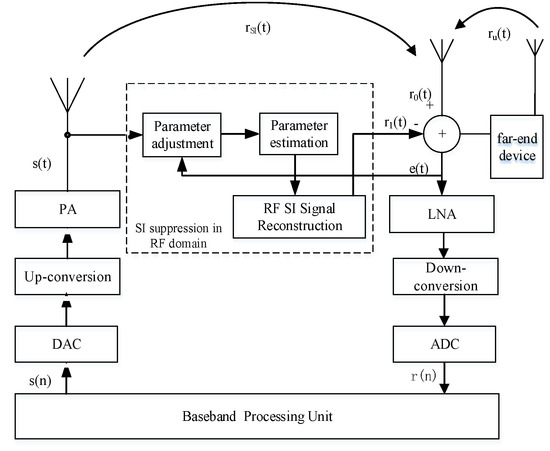
Figure 1.
Near-end transceiver model for the Co-frequency Co-time Full Duplex (CCFD) system.
For the transmitter of the near-end transceiver in the full duplex system, the output s(t) can be expressed as follows:
where is the near-end transmitted power, is carrier frequency, and is the initial phase. According to the transceiver model of the system, the signal received by the full duplex communication node entering the near-end is obtained as
The near-end SI signal can be specifically expressed as follows:
where is the impulse response of the SI channel, and are the amplitude attenuation factor and time delay of the SI channel, separately. Therefore, the SI signal can be represented as
In this paper, the SI signal in the RF domain of the near-end receiver of the full-duplex system is estimated using the DTV-LMS algorithm. The implementation process of this algorithm is described in detail in Section 3. The residual SI signal after SI cancellation in the RF domain (i.e., the error signal) can be expressed as
where is the estimated SI signal (i.e., the reconstructed SI signal).
2.2. Mathematical Model
The main mathematical principle of RF cancellation in a CCFD system is the composition of vectors [31]. The following notation is utilized in developing a mathematical model for the problem of SI cancellation in the RF domain addressed in this paper: s(t) is the near-end transmitting signal, is the same phase component as s(t), is the orthogonal component obtained by through a 90 degree phase shifter, is the estimated SI signal, r(t) is the near-end receiving signal, and e(t) is the error signal. Assuming that the SI signal in the RF domain is a vector in the space rectangular coordinate system, the signal can be cancelled by synthesizing another vector with the same information characteristics as the vector. As shown in Figure 2, the near-end transmitting signal s(t) is divided into two branches, and , after group delay, t. The delay block is the group delay of the estimate interference signal.
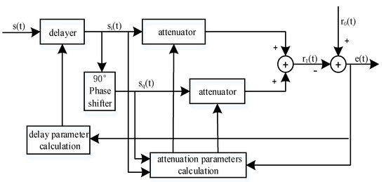
Figure 2.
Principle diagram of self-interference (SI) cancellation in the radio frequency (RF) domain.
Let , where T is the transpose of the matrix, and the weight vector is , that is the amplitude attenuation controlled by in-phase and orthogonal branch attenuator, which is used to adjust the amplitude and phase of . Therefore, the basic process of cancellation mentioned above can be expressed by
Equation (9) is the iteration formula for updating the weight vector of the LMS algorithm, where is a fixed step factor and is the step interval of feedback control. The above mentioned cancellation process, the amplitude of the in-phase component, and the orthogonal component can be changed by adjusting the value of , and then the SI signal can be reconstructed. Therefore, the weight vector is the key factor affecting the performance of SI cancellation. The adjustment of the weight vector based on the minimum mean square error (MMSE) criterion is expressed as
3. DTV-LMS Algorithm and Analysis
3.1. DTV-LMS Algorithm
As shown in Equation (9) above, in a classical LMS algorithm, is a fixed constant value whose convergence range is between [0, ], and is the maximum eigenvalue of the autocorrelation matrix of the input signal. The convergence speed of the LMS algorithm became faster with an increase of , but at the same time, it produces a problem by increasing SSM. An optimized LMS algorithm called the DTV-LMS algorithm is proposed in this paper. This algorithm makes the value of the step factor change over time (from large to small) to reduce SSM. Based on the iterative formula in the reference [20,21], we make further improvements the weight and step updating formulas of the DTV-LMS algorithm, as given in Equations (11) and (12), respectively:
where α, β are constants, which are used to control the step-size in order to accelerate the convergence speed while keeping a low steady-state error; ρ is also a constant and can solve the numerical problem that a minimal value exists when S(t) is too small.
The autocorrelation of the error signal is used from Formula (11) to reduce the impact of burst impulse noise interference, thereby improving ICR and the cancellation performance. The step updating equation uses the arctangent function to establish a new non-linear relationship with the time parameters. Compared to the sigmoid function and hyperbolic tangent function used in references, the simulation results are shown in Figure 3.
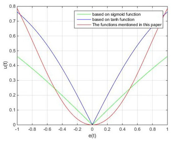
Figure 3.
The curves of the step-size characteristics.
From the curve shown in Figure 3, it is obvious that when the error factor is close to zero, the sigmoid function and tanh function will change dramatically, and the small error changes will result in large step size changes. The optimized algorithm proposed in this paper overcomes this shortcoming very well, and changes slowly when approaches zero, so that the adaptive weight vector value of the algorithm is closer to the actual value when it reaches a steady state.
From Equation (11), we can see that the updating of is influenced by the statistical characteristics of the near-end transmitting signal, and the adjustment of the weight vector is controlled by the step factor. That is to say, the algorithm uses the statistical characteristics of the transmitting signal to realize an effective adjustment of the weight.
In addition, we adjust the coefficients α, β to change the convergence performance. The curves of the relationship between and are shown in Figure 4 and Figure 5, with a change in the values of and , respectively. From the two figures, we can see when the slope gets larger, the step causes a mutation just as the error approaches 0, so ‘’ should not be too large. Similarly, ‘’ also needs to be selected reasonably.
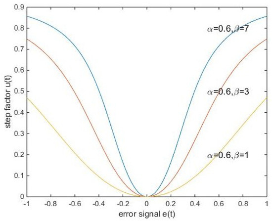
Figure 4.
The variation of curves; when = 0.6, changes.
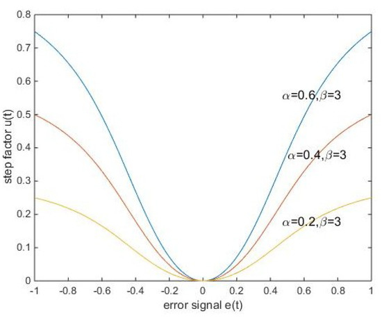
Figure 5.
The variation of curves; when = 0.3, changes.
According to the model of the CCFD system and the structure of RF cancellation mentioned in Section 2, the detailed steps of the SI cancellation method in the RF domain are given as follows:
- Step 1.
- The group delay time of the transmitted and received signals is estimated by the training sequence.
- Step 2.
- The optimal values of parameters α, β are determined according to various parameters of the CCFD system model.
- Step 3.
- Give the initial value to the weight vector , assuming e(t) = r0(t), when .
- Step 4.
- The μ(t) is calculated at intervals of time ∆t, and the weights are updated while adjusting the gains of the two in-phase and orthogonal branches.
- Step 5.
- Calculate the real-time error signal e(t).
- Step 6.
- Return to (4).
3.2. Performance Analysis
In a full duplex system, the SI signals at the near-end transceivers and the useful signals at the far-end are independent of each other. In order to make the analysis more convenient, assuming that the error of time delay is 0, the coefficients of the in-phase component and the orthogonal component corresponding to the SI signal are, respectively, , . The in-phase and orthogonal components are wide stationary random signals with a mean of 0. Assuming that their power is and the power of the useful signal is at the far end, the mean square of the error signal during can be represented by
where is the mean power of AWGN, and the weight vector formula is further simplified as
where is the weight of the real SI signal, and I is the identity matrix. Combining Formula (13) and (14), (15) can be obtained as follows:
The initial value to the weight vector . Assuming , according to Equation (15), the relationship between the mean square error (MSE) of the nth iteration and the initial MSE can be obtained as follows:
It can be seen that the convergence conditions of the above equation are , . Due to generally being very small, the condition for the convergence can be simplified as , and then we can express ,which is consistent with the convergence conditions of the classical LMS algorithm given above. It can be seen from Equation (16) that the convergence of the algorithm is determined by the trend of the cumulative product value in the error convergence function.
Let the convergence factors of the LMS algorithm and the DTVLMS algorithm be . According to Equation (16), we can obtain as
It can be seen from the above two formulas, compared with the convergence factors of the traditional fixed-step LMS algorithm, that the convergence speed of the DTV-LMS algorithm is almost independent of the power of the near-end transmitted signal in the RF domain, which can effectively avoid the interference of the gradient noise amplification. In addition, by using the correlation value of the error signal to adjust the step size, the algorithm can take into account the performance of the convergence speed and error. At the same time, the problem of intermittent communication or burst noise interference by relying only on the time parameter can also be effectively solved.
According to reference [24], the equation for ICR is , where and is the power of the near-end SI signal before and after the SI cancellation in RF domain, respectively. Let . When , the MSE of the DTV-LMS algorithm tends to be stable, and Formula (16) can be simplify as
Because , when K→∞, , and we can get the formula of MSE as
Thus, the ICR of the DTV-LMS algorithm can be given as
According to the above equation, ICR will be applied to the simulation experiment in the next section, and its performance will be verified from the simulation results.
4. Simulation and Result Analysis
4.1. Simulation Parameter Setting
In this section, we make use of a MATLAB simulation to test the performance of the convergence speed, ICR, tracking speed, and so on. The conditions of the computer simulation parameters are:
- Simulating modulation using quadrature phase shift keying (QPSK) with a transmission rate of 10 Mbps and a carrier frequency of 2.1 GHz, regardless of the nonlinear and ADC quantization noise effects;
- Setting the noise limit of the received channel to −95 dBm by referring to reference [25]; the power of desired signal is −85 dBm, the SI signal is −10 dBm (i.e., the modulated channel ISR = 75 dB), and the SNR = 10 dB;
- The step interval is . Let t = n, and change the phase of the SI signal at the 500th (i.e., t = 15 ms) iteration;
- Extract 1000 sampling points and perform 200 statistically independent simulation experiments.
The improved LMS algorithm proposed in this paper is compared with the existing RF cancellation algorithms of SVSLMS [20], VSSLMS [19], and MVSSLMS [21]. Refer to the parameter setting principle of reference in [19,20,21,29], as the parameters of these algorithms are selected to produce a comparable level of mis-adjustments, assuming that the delay estimation error is 0, and the power value of the reference signal is 0 dBm [30], and give the specific parameters of the four algorithms as shown in Table 1.

Table 1.
The corresponding parameter value of each algorithm.
4.2. Results Analysis
From the simulation curves of Figure 6 and Figure 7, we can see that in terms of convergence speed under the condition of parameter 1, The DTV-LMS algorithm can reach a convergence state approximately during its 25th iteration. The MVSSLMS algorithm can reach a convergence state at about the 36th iteration. The VSSLMS algorithm and SVSLMS algorithm can reach convergence states at about the 70th iteration and the 120th iteration, respectively. Similarly, under the conditions of parameter 2, although their convergence speeds differ slightly, the convergence speed of the DTV-LMS algorithm proposed in this paper is obviously faster than the other three compared algorithms. When the phase change of the signal (i.e., the 500th iteration, the tracking, and the SSM performance of the DTV-LMS and the SVSLMS algorithms) is better than that of the other two algorithms, they can quickly converge again. However, the computational complexity of the DTV-LMS algorithm is lower than that of the SVSLMS algorithm. Thus, the algorithm proposed in this paper is slightly better.
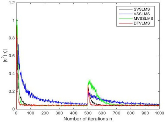
Figure 6.
The curves of the algorithm convergence in parameter 1.
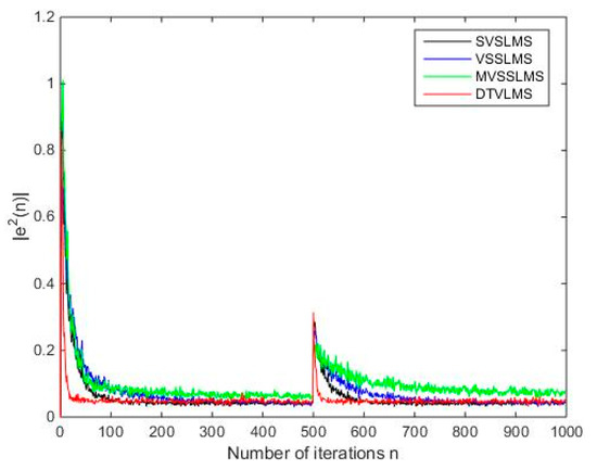
Figure 7.
The curves of the algorithm convergence in parameter 2.
It can be seen from the curve of the ICR shown in Figure 8 and Figure 9 that under the condition of parameter 1, the final ICR values of the SVSLMS, MVSSLMS, and VSSLMS algorithms are 74.98 dB, 74.76 dB, and 74.15 dB, respectively; their ICR are close to each other. The final ICR value of the DTV-LMS algorithm proposed in this paper is 78.21 dB, which increased by at least 5 dB compare to the other three algorithms. Under the condition of parameter 2, the ICR values of DTV-LMS, SVSLMS, MVSSLMS, and VSSLMS are 79.96 dB, 77.03 dB, 78.12 dB, and 75.65 dB, respectively, and the ICR value of the proposed algorithm is still the highest. When the phase suddenly changes its signal (i.e., when the 15 ms signal from the graph of the curve changes), we can see that the DTV-LMS algorithm clearly achieves its final stable ICR value faster than the other three compared algorithms—that is to say, the algorithm proposed in this paper can track and adapt to channel changes in a short time, and return to the stable state before channel mutation. This algorithm is verified to have a good adaptive channel tracking capability.
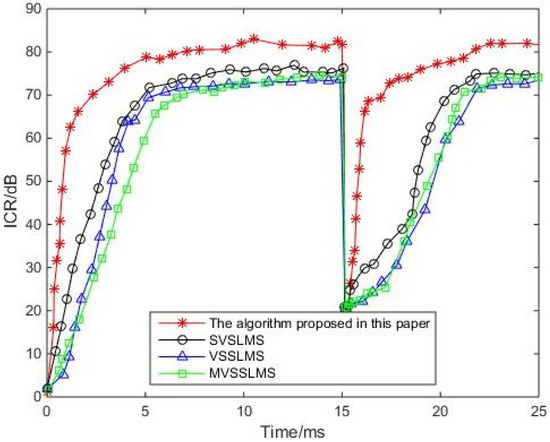
Figure 8.
The curves of the algorithm’s interference cancellation ration (ICR) in parameter 1.
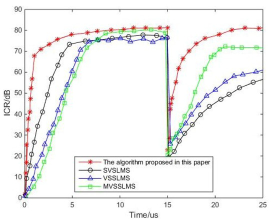
Figure 9.
The curves of the algorithm’s ICR in parameter 2.
It can be seen from the curve of the ICR shown in Figure 8 and Figure 9 that under the condition of parameter 1, the final ICR values of the SVSLMS, MVSSLMS, and VSSLMS algorithms are 74.98 dB, 74.76 dB, and 74.15 dB, respectively; their ICR are close to each other. The final ICR value of the DTV-LMS algorithm proposed in this paper is 78.21 dB, which increased by at least 5 dB compare to the other three algorithms. Under the condition of parameter 2, the ICR values of DTV-LMS, SVSLMS, MVSSLMS, and VSSLMS are 79.96 dB, 77.03 dB, 78.12 dB, and 75.65 dB, respectively, and the ICR value of the proposed algorithm is still the highest. When the phase suddenly changes its signal (i.e., when the 15 ms signal from the graph of the curve changes), we can see that the DTV-LMS algorithm clearly achieves its final stable ICR value faster than the other three compared algorithms—that is to say, the algorithm proposed in this paper can track and adapt to channel changes in a short time, and return to the stable state before channel mutation. This algorithm is verified to have a good adaptive channel tracking capability.
In order to further explore the influence of intervals of time ∆t on SI cancellation in the RF domain of the DTV-LMS algorithm, we changed the step interval, and other parameters remain unchanged under the condition of parameter 1. As shown in Figure 10, we can see that the convergence speed of the DTV-LMS algorithm slows down when the time interval for the feedback control in the system is larger, but it has no effect on the final ICR value of the DTV-LMS algorithm.
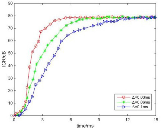
Figure 10.
Impact of the time interval on ICR.
5. Conclusions
In this paper, an optimized LMS algorithm based on the attenuation of the step of the convergence parameters is proposed, and we called this novel algorithm the DTV-LMS algorithm. The DTV-LMS algorithm can solve the problem of the strong SI of RF domain in the CCFD system by cooperatively controlling the autocorrelation values between the time factor and the error signal to update the step size of the algorithm and provide a better quality of service for 5G communication networks. The proposed DTV-LMS algorithm is compared with the SVSLMS, MVSSLMS, VSSLMS algorithms and used to verify the superiority of the proposed algorithm by analyzing the convergence speed, the ICR, and the channel tracking capability among these algorithms. The final ICR value of the DTV-LMS algorithm proposed in this paper is 78.21 dB approximately, and the final ICR values of the SVSLMS, MVSSLMS, and VSSLMS algorithms are about 74.98 dB, 74.76 dB, and 74.15 dB. Meanwhile, the convergence speed of the algorithm is also obviously improved compared to the other reference algorithms mentioned in this paper, according to the experimental results. The theoretical analysis and simulation results show that the proposed algorithm achieves a good balance between convergence speed and SSE, which can maintain a small value of SSE at a faster convergence speed, and it also has a good channel tracking capability when dealing with burst noise interference. Therefore, it can be better applied to a 5G wireless communication environment.
However, we experimented with simulations under ideal conditions in this study—for example, the effects of nonlinear interference are not considered, so it has certain limitations. We are committed to researching and solving possible problems in real-life scenarios in future work. In addition, our test cases also have limitations, and we should enrich our test cases in the next work. Since some residual SI signals are still not eliminated after SI cancellation at the RF domain, we will also research how to eliminate residual SI completely in the digital domain in our next work. All in all, we still have many things to improve, and we will work hard to find the perfect way to solve them in our future work.
Author Contributions
Z.-Y.S. conceptualized the study and provided resources. Y.-J.Z. designed the experiments, conducted data analyses, wrote the original draft of the manuscript. Z.-Y.S. and Y.-J.Z. reviewed and improved the manuscript.
Funding
This research received no external funding.
Conflicts of Interest
The authors declare that there is no conflict of interests regarding the publication of this article.
References
- Hong, S.; Brand, J.; Choi, J.I.; Jain, M.; Mehlman, J. Applications of Self-Interference Cancellation in 5G and Beyond. IEEE Commun. Mag. 2014, 52, 114–121. [Google Scholar] [CrossRef]
- Aly, R.M.; Zaki, A.; Badawi, W.K.; Aly, M.H. Time Coding OTDM MIMO System Based on Singular Value Decomposition for 5G Applications. Appl. Sci. 2019, 9, 2691. [Google Scholar] [CrossRef]
- Panwar, N.; Sharma, S.; Singh, A.K. A Survey on 5G: The Next Generation of Mobile Communication. Phys. Commun. 2016, 18, 64–84. [Google Scholar] [CrossRef]
- Akyildiz, I.F.; Nie, S.; Lin, S.C.; Chandrasekaran, M. 5G Roadmap: 10 Key Enabling Technologies. Comput. Netw. 2016, 106, 17–48. [Google Scholar] [CrossRef]
- Liu, G.; Yu, F.R.; Ji, H.; Leung, V.C.M.; Li, X. In-Band Full-Duplex Relaying for 5G Cellular Networks with Wireless Virtualization. IEEE Netw. 2015, 29, 54–61. [Google Scholar] [CrossRef]
- Li, G.; Sun, C.; Zhang, J.; Jorswieck, E.; Xiao, B.; Hu, A. Physical Layer Key Generation in 5G and Beyond Wireless Communications: Challenges and Opportunities. Entropy 2019, 21, 497. [Google Scholar] [CrossRef]
- Zhao, H.; Wang, J.; Tang, Y. Performance Analysis of RF Self-Interference Cancellation in Broad Band Full Duplex Systems. In Proceedings of the 2016 IEEE International Conference on Communications Workshops (2016 ICC), Kuala Lumpur, Malaysia, 23–27 May 2016. [Google Scholar]
- Zhang, Z.; Long, K.; Uasilakos, A.V. Full-duplex wireless communications: Challenges, solutions, and future research diretions. Proc. IEEE. 2016, 104, 1369–1409. [Google Scholar] [CrossRef]
- Atapattu, S.; He, Y.; Dharmawansa, P.; Evans, J. Impact of residual self-interference and direct-link interference on full-duplex relays. In Proceedings of the IEEE International Conference on Industrial & Information Systems, Peradeniya, Sri Lanka, 15–16 December 2017. [Google Scholar]
- Debaillie, B.; Broek, D.J.; Lavin, C. Analog/RF Solutions Enabling Compact Full-Duplex Radios. IEEE J. Sel. Areas Commun. 2014, 32, 1662–1673. [Google Scholar] [CrossRef]
- Do, D.; Van Nguyen, M.; Hoang, T.; Lee, B.M. Exploiting Joint Base Station Equipped Multiple Antenna and Full-Duplex D2D Users in Power Domain Division Based Multiple Access Networks. Sensors. 2019, 19, 2475. [Google Scholar] [CrossRef]
- Ro, J.; Park, S.; Song, H. An Interference Cancellation Scheme for High Reliability Based on MIMO Systems. Appl. Sci. 2018, 8, 466. [Google Scholar]
- Xia, W.; Xia, X.; Li, H.; Liu, W.; Hu, J.; He, Z. A noise-constrained distributed adaptive direct position determination algorithm. Signal Process. 2017, 135, 9–16. [Google Scholar] [CrossRef]
- Sakai, M.; Lin, H.; Yamashita, K. Self-Interference Cancellation in Full-Duplex Wireless with IQ Imbalance. Phys. Commun. 2016, 18, 2–14. [Google Scholar] [CrossRef]
- Kim, B.; Yoon, J. Modified LMS Strategies Using Internal Model Control for Active Noise and Vibration Control Systems. Appl. Sci. 2018, 8, 1007. [Google Scholar]
- Vázquez, Á.A.; Maya, X.; Avalos, J.G.; Sánchez, G.; Sánchez, J.C.; Pérez, H.M.; Sánchez, G. A Time-Efficient Method for Determining an Optimal Scaling Factor and the Encoder Resolution in the Multichannel FXECAP-L Algorithm with Evolving Order for Active Noise Control. Appl. Sci. 2019, 9, 560. [Google Scholar] [CrossRef]
- Le-Ngoc, T.; Masmoudi, A. Full-Duplex Wireless Communications Systems: Self-Interference Cancellation; Springer: Cham, Switzerland, 2017; Volume 54, pp. 1001–1006. [Google Scholar]
- Wang, J.; Zhao, H.; Tang, Y. A RF Adaptive Least Mean Square Algorithm for Self-interference Cancellation in Co-frequency Co-time Full Duplex Systems. In Proceedings of the 2014 IEEE International Conference on Communications (ICC), Sydney, NSW, Australia, 10–14 June 2014. [Google Scholar]
- Lee, H.S.; Kim, S.E.; Lee, J.W. A Variable Step-Size Diffusion LMS Algorithm for Distributed Estimation. IEEE Trans. Signal Process. 2015, 63, 1808–1820. [Google Scholar] [CrossRef]
- Zou, Y.Z.; Xin, X.; Zhang, J.Y. Improved Time-Varying Step-Size NLMS Algorithm for RF Self-Interference Cancellation in Full-Duplex. J. Signal Process. 2017, 32, 787–791. [Google Scholar]
- Ao, W.; Xiang, X.Q.; Zhang, Y.P. A New Variable Step Size LMS Adaptive Filtering Algorithm. In Proceedings of the International Conference on Computer Science & Electronics Engineering, Hangzhou, China, 23–25 March 2012. [Google Scholar]
- Cheng, W.; Zhang, X.; Zhang, H. Optimal Dynamic Power Control for Full-Duplex Bidirectional-Channel Based Wireless Networks. In Proceedings of the IEEE INFOCOM, Turin, Italy, 14–19 April 2013. [Google Scholar]
- Vaňuš, J.; Styskala, V. Application of optimal settings of the LMS adaptive filter for speech signal processing. In Proceedings of the International Multiconference on Computer Science & Information Technology, Wisla, Poland, 18–20 October 2010. [Google Scholar]
- Masmoudi, A.; Le-Ngoc, T. Channel Estimation and Self-Interference Cancellation in Full-Duplex Communication Systems. IEEE Trans. 2017, 66, 321–334. [Google Scholar]
- Dinesh, B.; Emily, M.; Sachin, K. Full Duplex Radios. ACM SIGCOMM Comput. Commun. Rev. 2013, 43, 375–386. [Google Scholar]
- Melissa, D. Full-Duplex Wireless: Design, Implementation and Characterization. Ph.D. Thesis, Rice University, Houstin, TX, USA, 2012. [Google Scholar]
- Lu, H.T.; Shao, S.H.; Tang, Y.X. Self-Mixed Self-Interference Analog Cancellation in Full-Duplex Communication. Sci. China Inf. Sci. 2016, 59, 042303. [Google Scholar] [CrossRef]
- Angelakis, V.; Chen, L.; Yuan, D. Optimal and Collaborative Rate Selection for Interference Cancellation in Wireless Networks. IEEE Commun. Lett. 2011, 15, 819–821. [Google Scholar] [CrossRef]
- D’Andreagiovanni, F.; Mannino, C.; Sassano, A. GUB Covers and Power-Indexed Formulations for Wireless Network Design. Manag. Sci. 2013, 59, 142–156. [Google Scholar] [CrossRef]
- Al-Zahrani, A.Y. A Game Theoretic Interference Management Scheme in Full Duplex Cellular Systems under Infeasible QoS Requirements. Future Internet. 2019, 11, 156. [Google Scholar] [CrossRef]
- Qiao, G.; Gan, S.; Liu, S.; Ma, L.; Sun, Z. Digital Self-Interference Cancellation for Asynchronous In-Band Full-Duplex Underwater Acoustic Communication. Sensors 2018, 18, 1700. [Google Scholar] [CrossRef]
© 2019 by the authors. Licensee MDPI, Basel, Switzerland. This article is an open access article distributed under the terms and conditions of the Creative Commons Attribution (CC BY) license (http://creativecommons.org/licenses/by/4.0/).