Sampling Based on Kalman Filter for Shape from Focus in the Presence of Noise


Abstract

1. Introduction
2. Related Work
2.1. Shape from Focus
2.2. Focus Measures
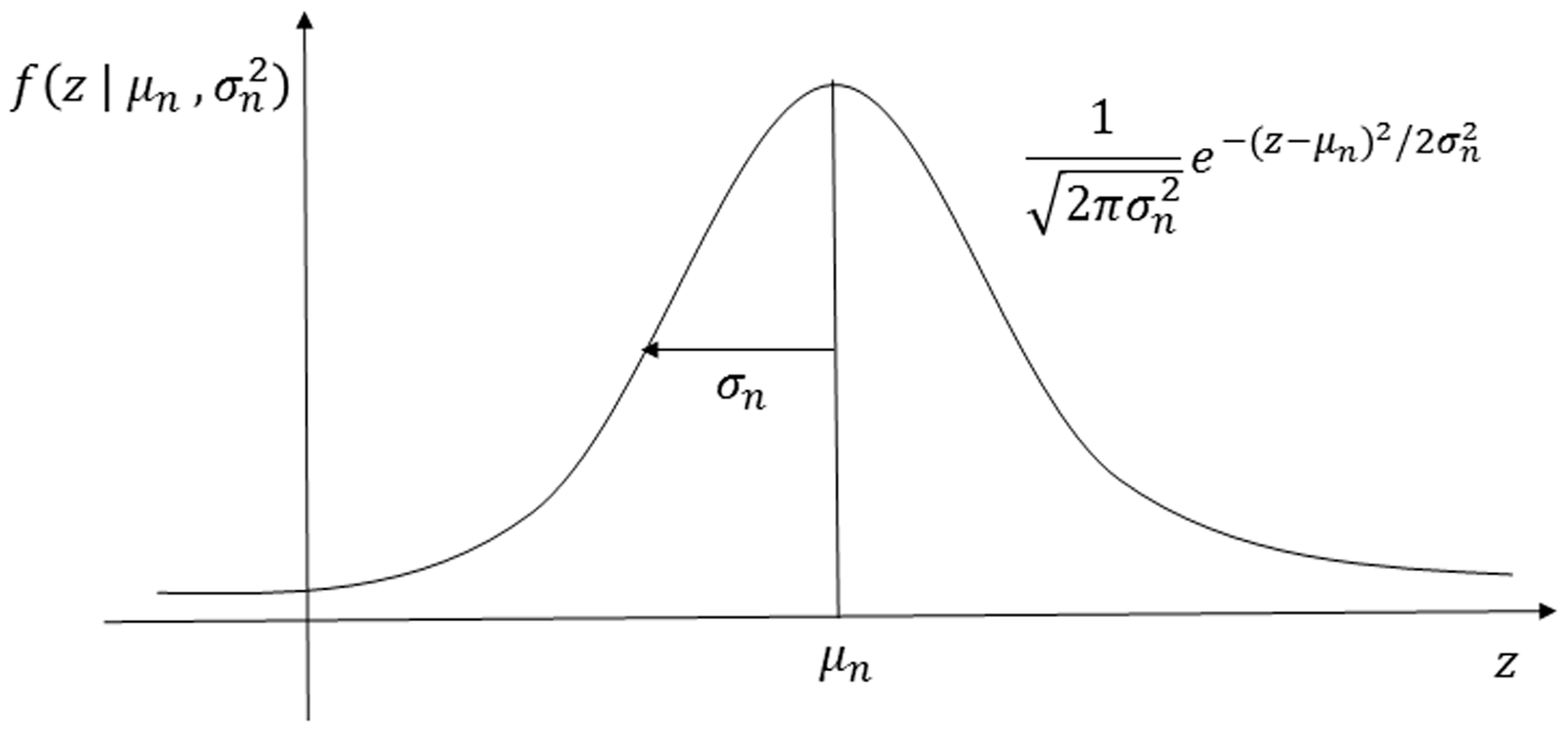
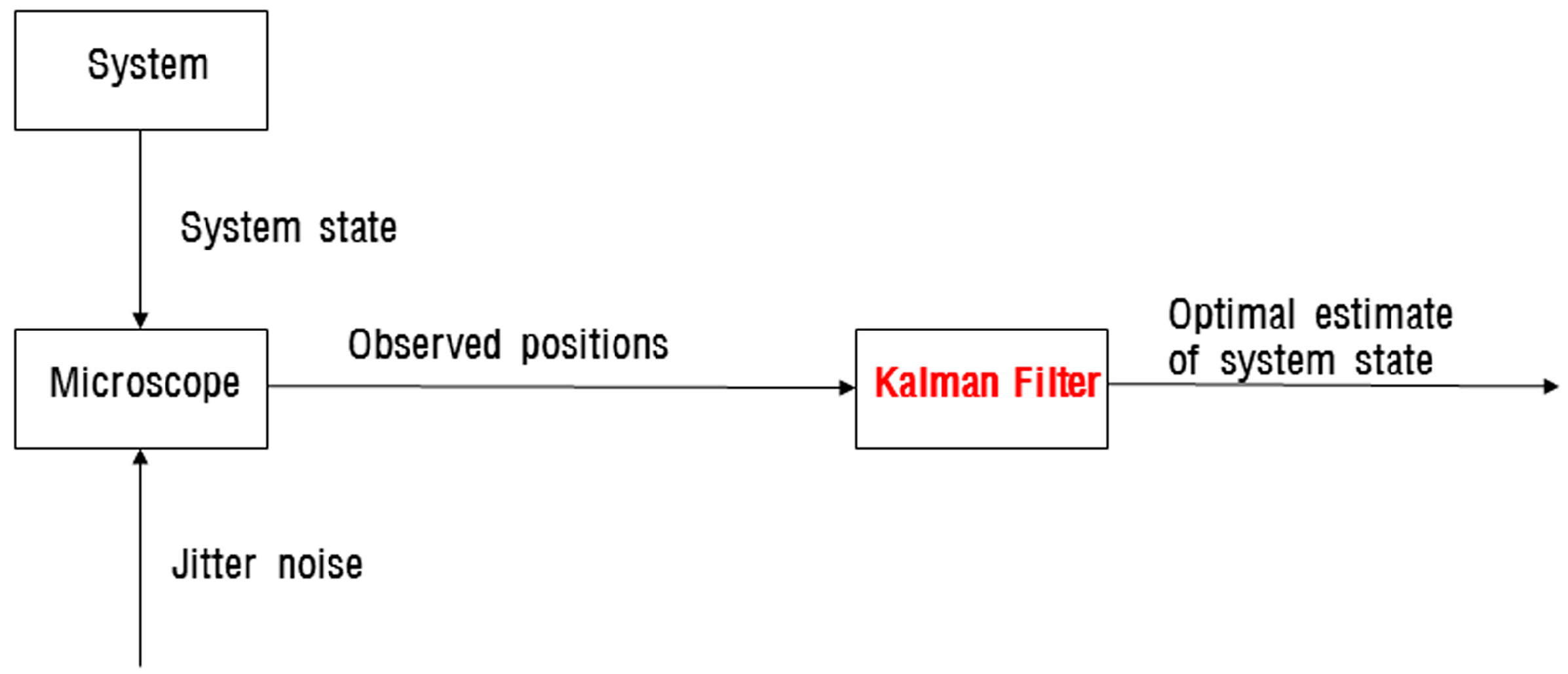
3. Noise Modeling
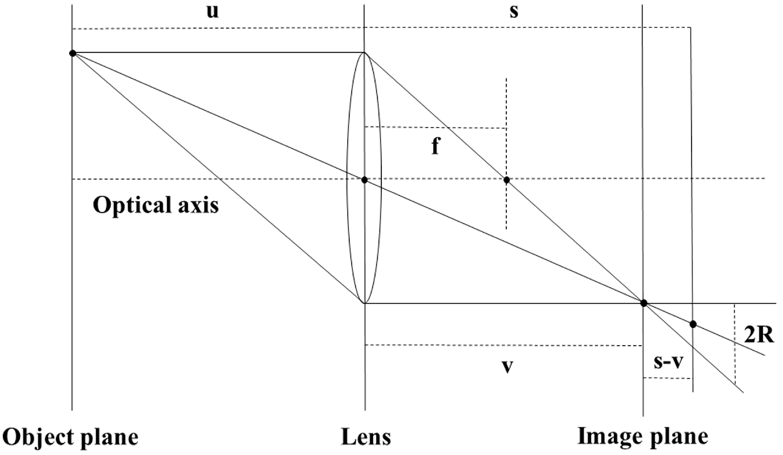
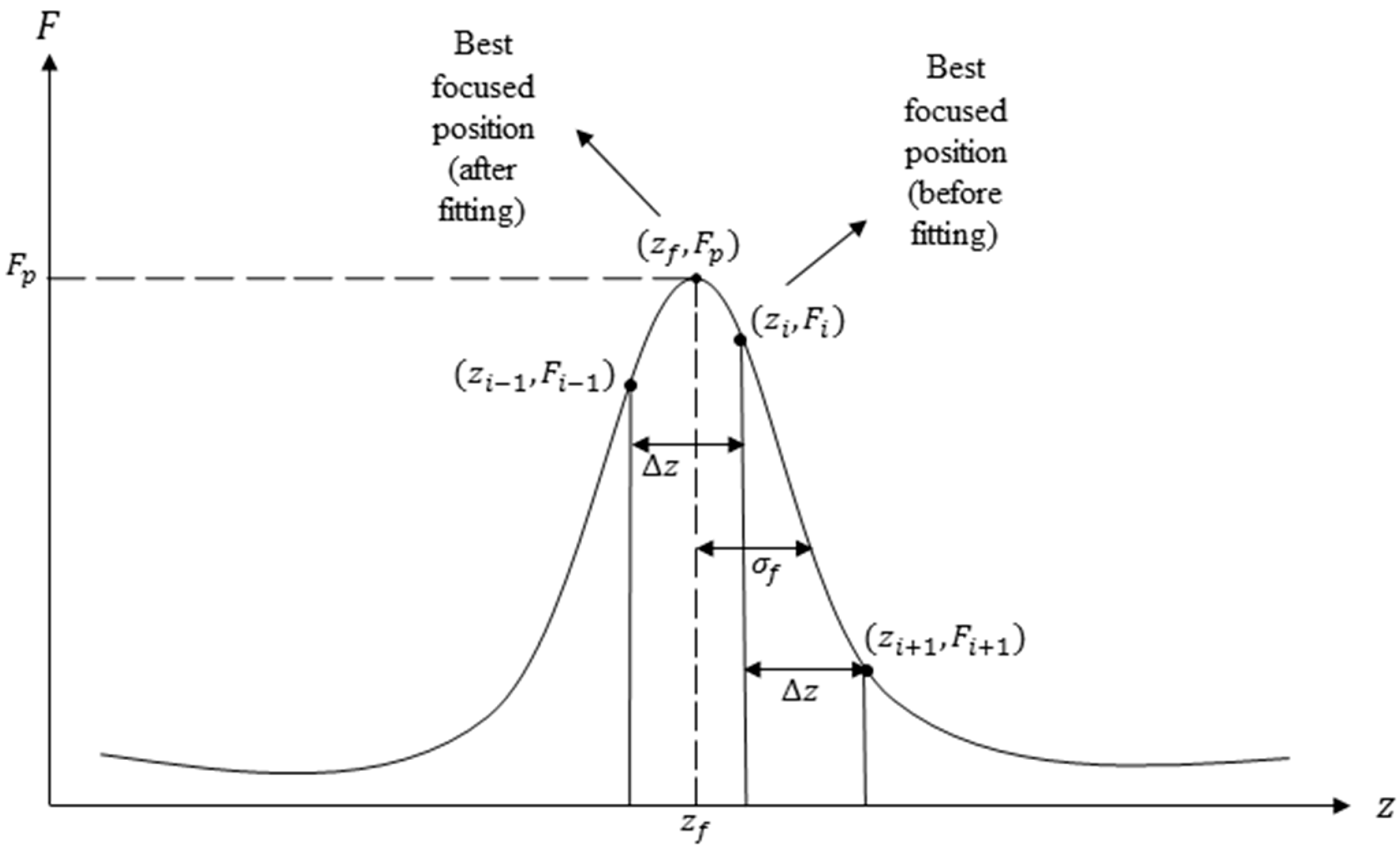
4. Focus Curve Modeling
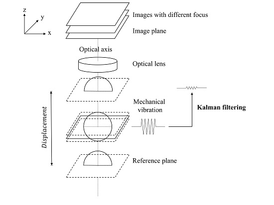
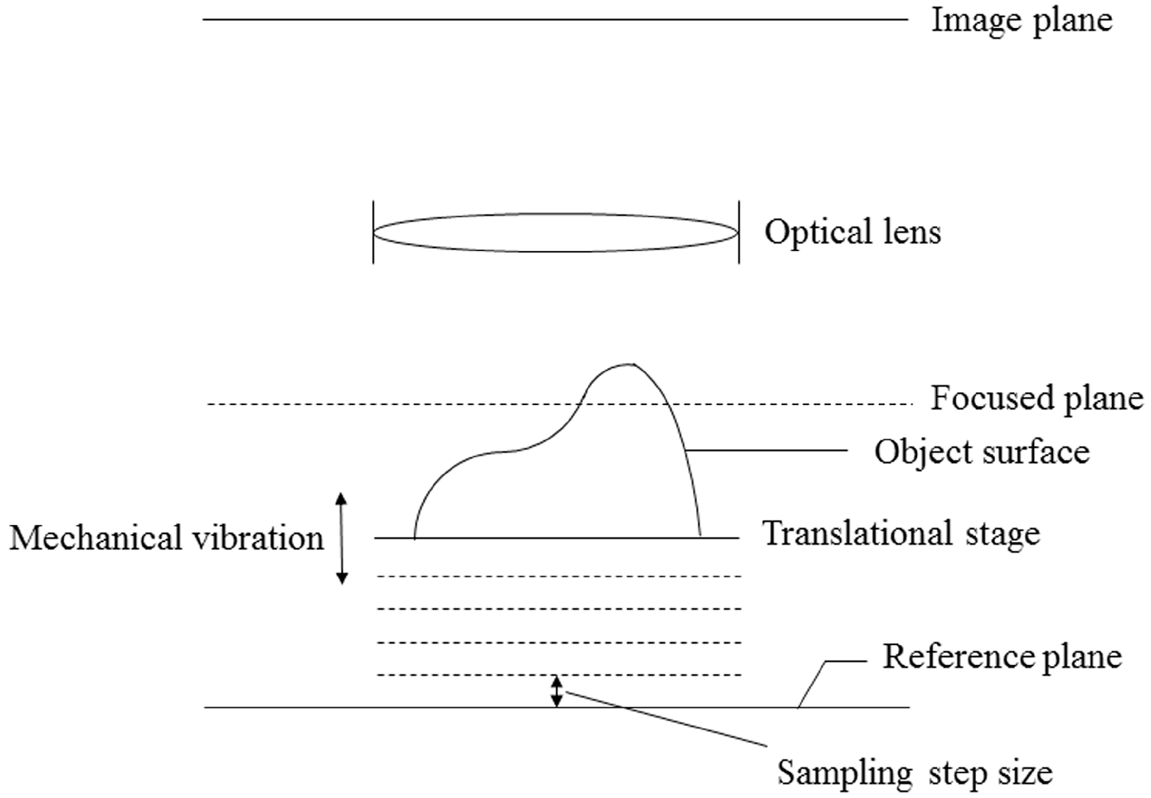
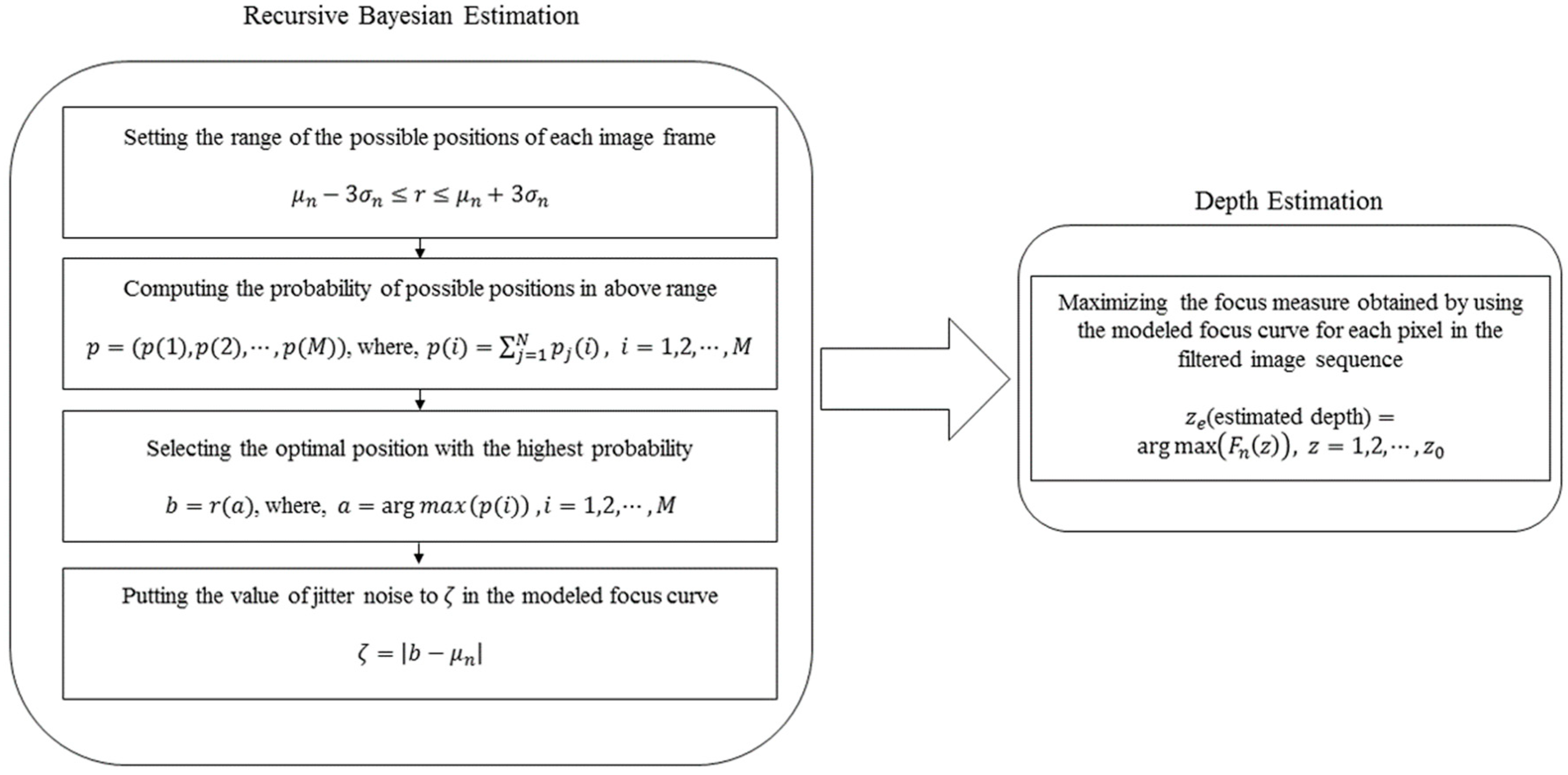
5. Proposed Method
| Algorithm 1 Computing optimal position of each image frame and remaining jitter noise |
| 1: procedure Optimal position & remaining jitter noise 2: Set initial position of image frame with observed position 3: Initialize variance of position of image frame to variance of jitter noise 4. for do Total number of iterations of Kalman filter 5: Compute Kalman gain 6: Correct variance of position of image frame 7: Update position of image frame 8: Compute remaining jitter noise 9: end for 10: end procedure |
6. Results and Discussion
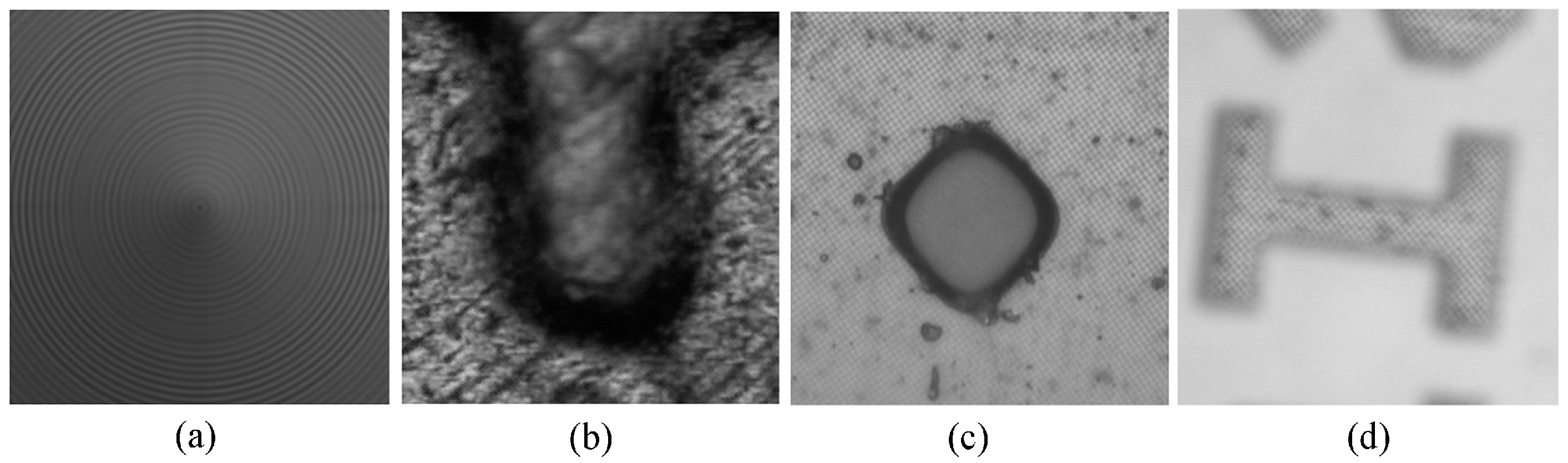
6.1. Image Acquisition and Parameter Setting
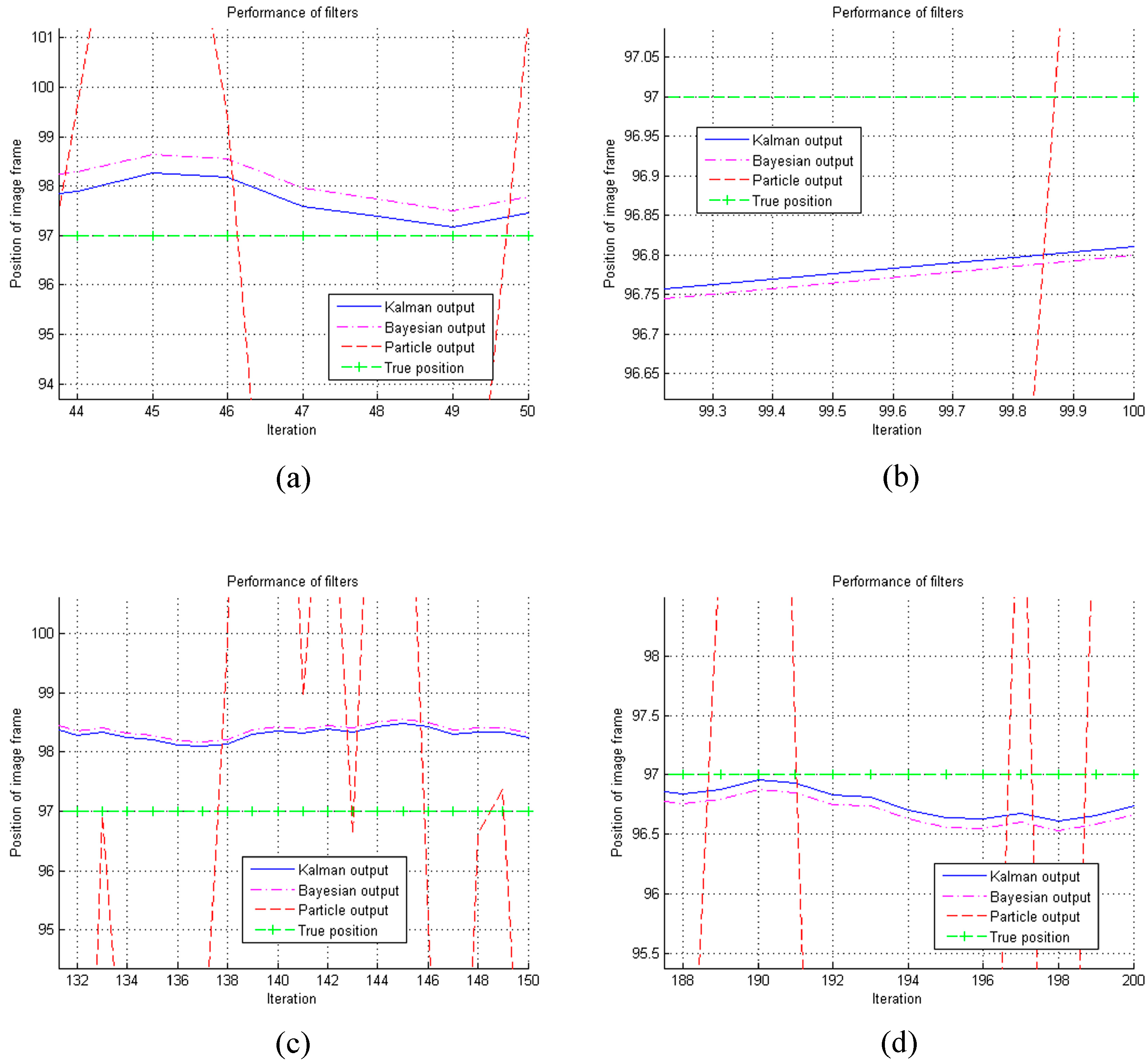
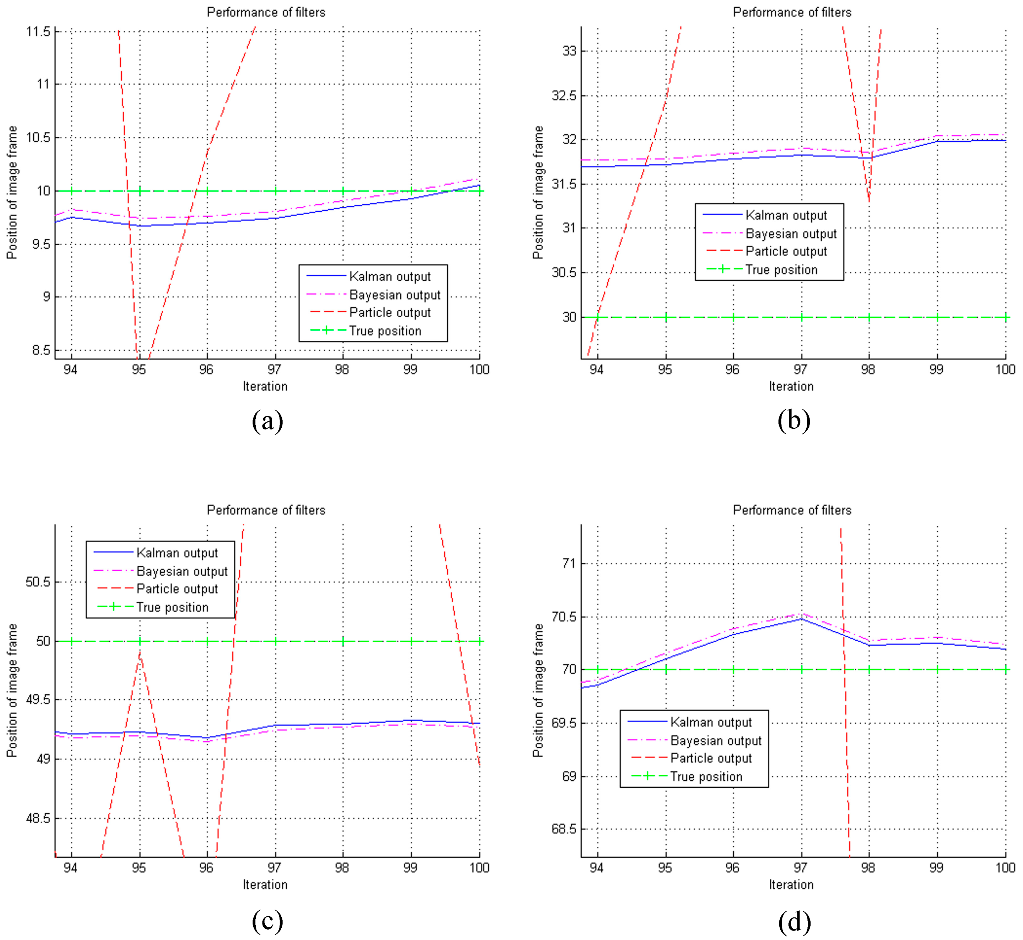
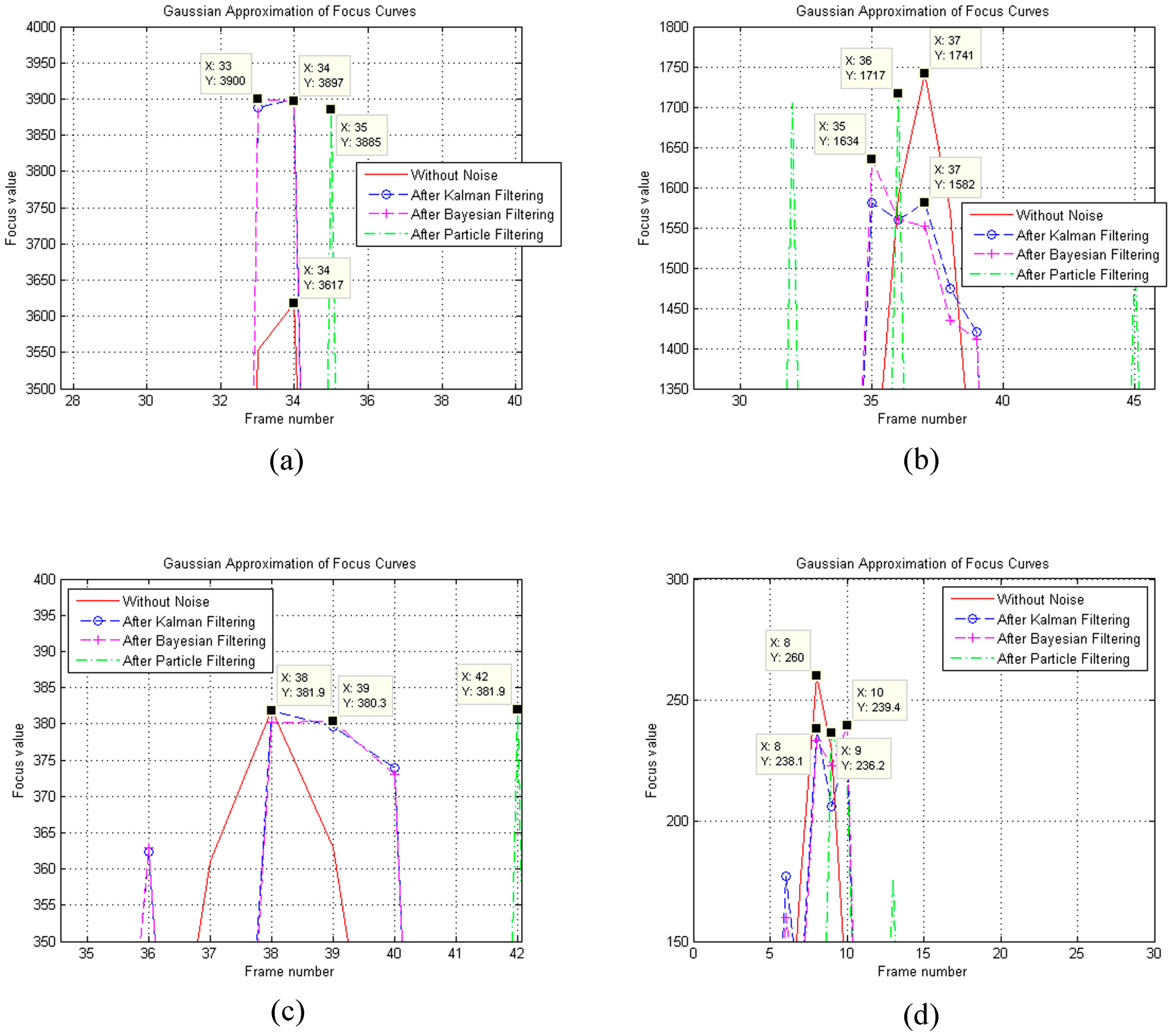
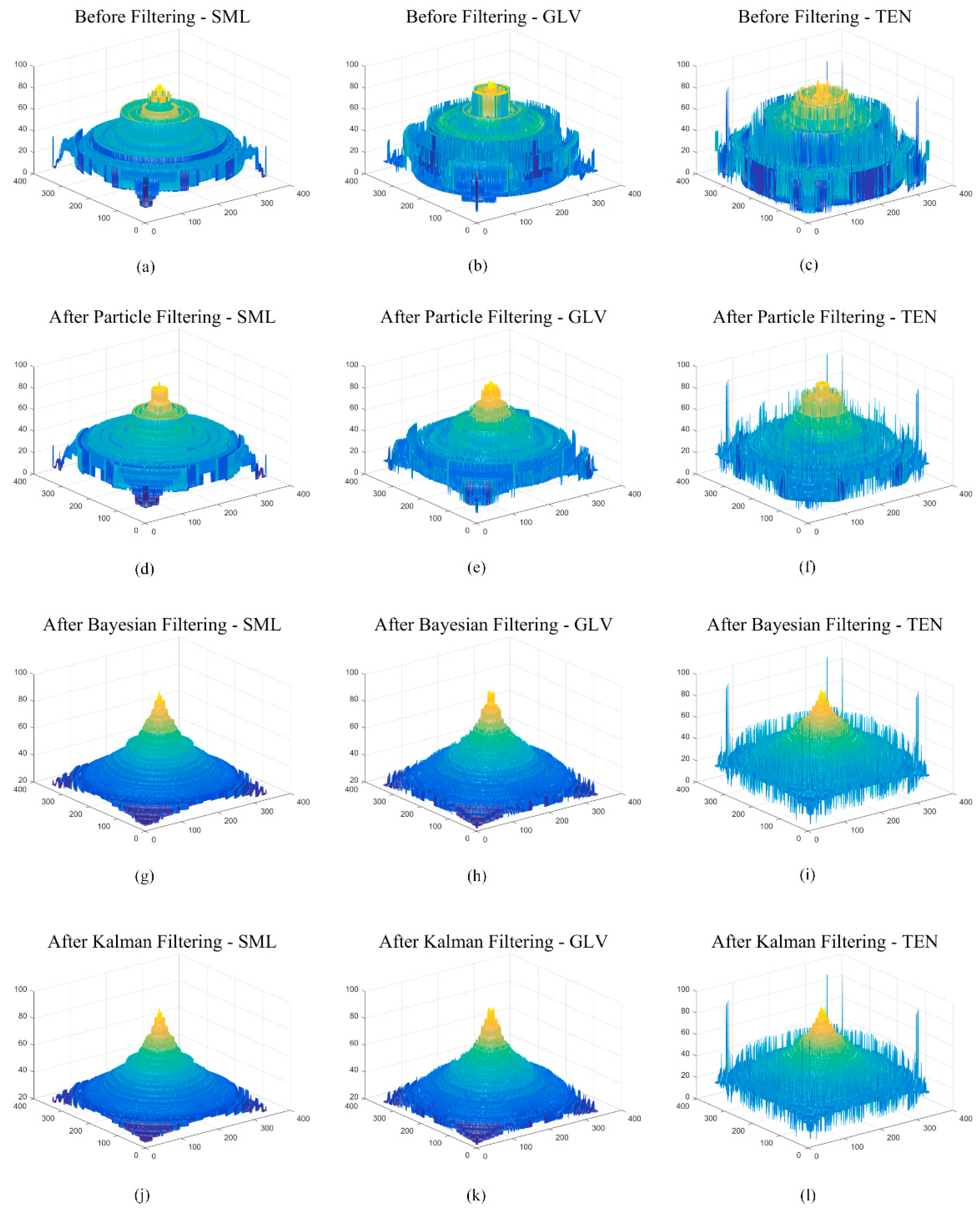
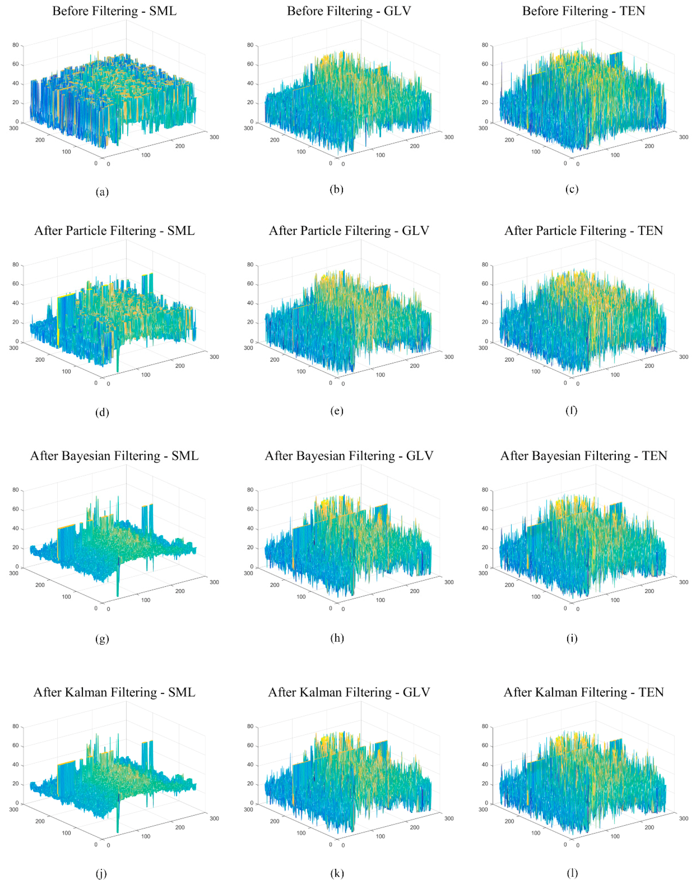
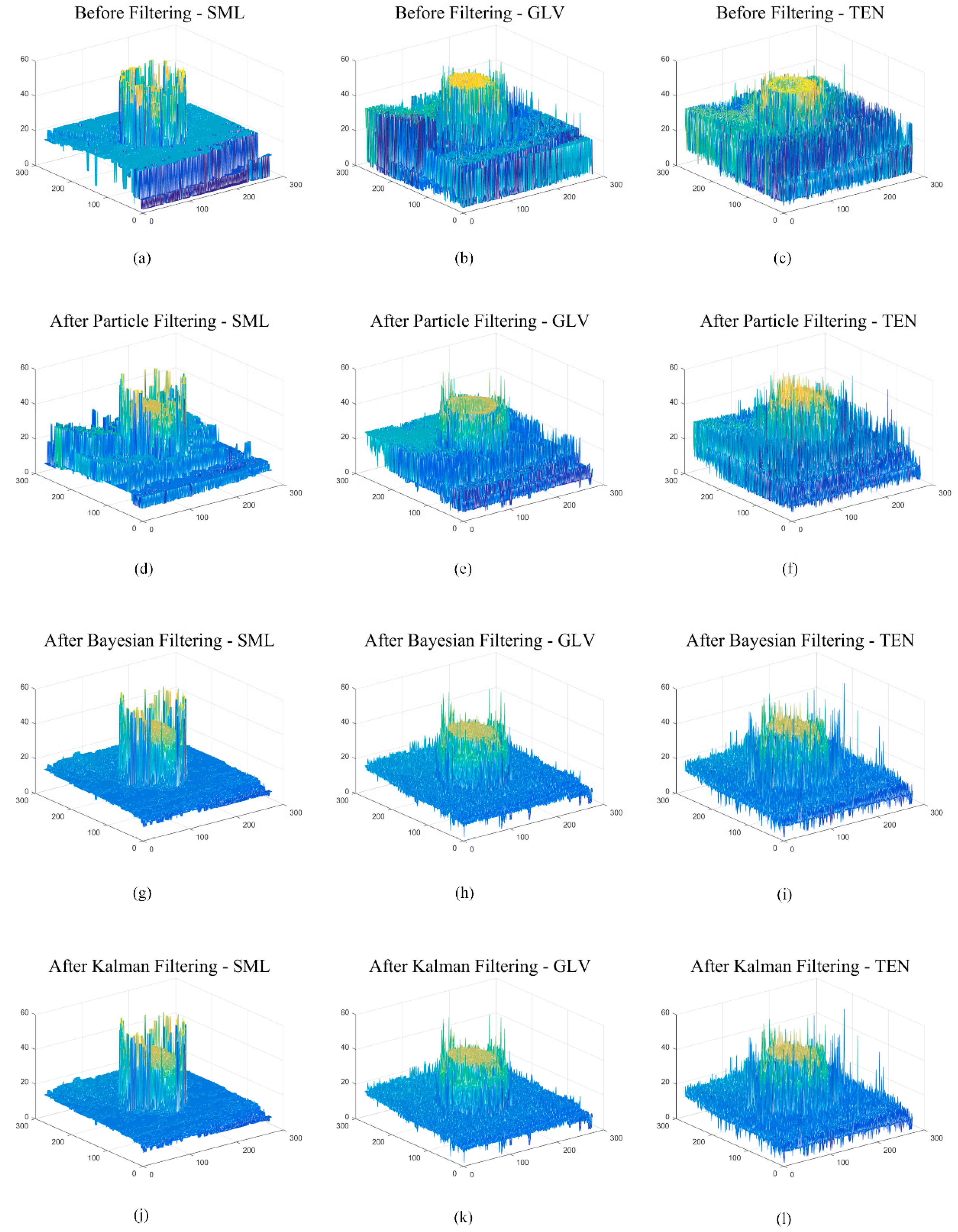
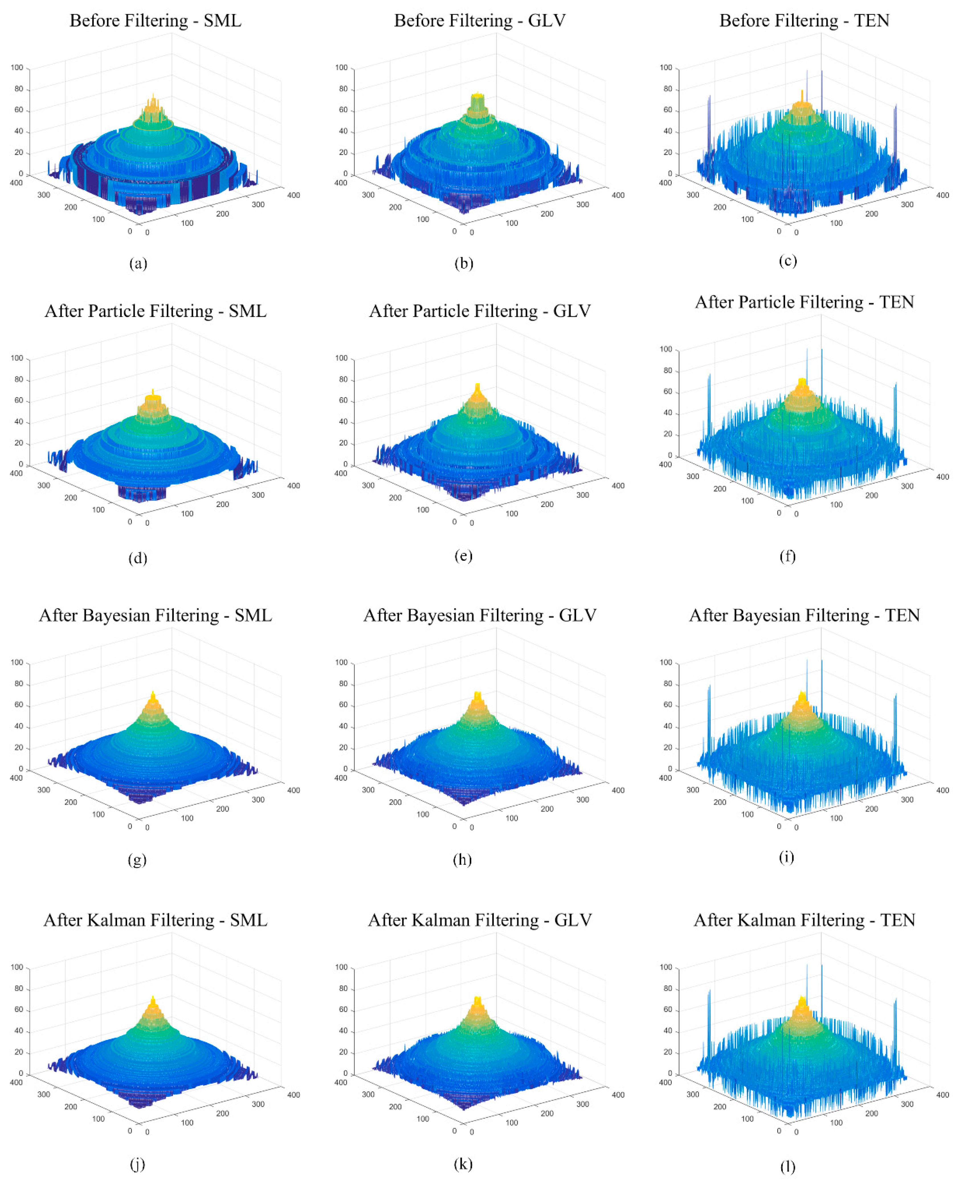
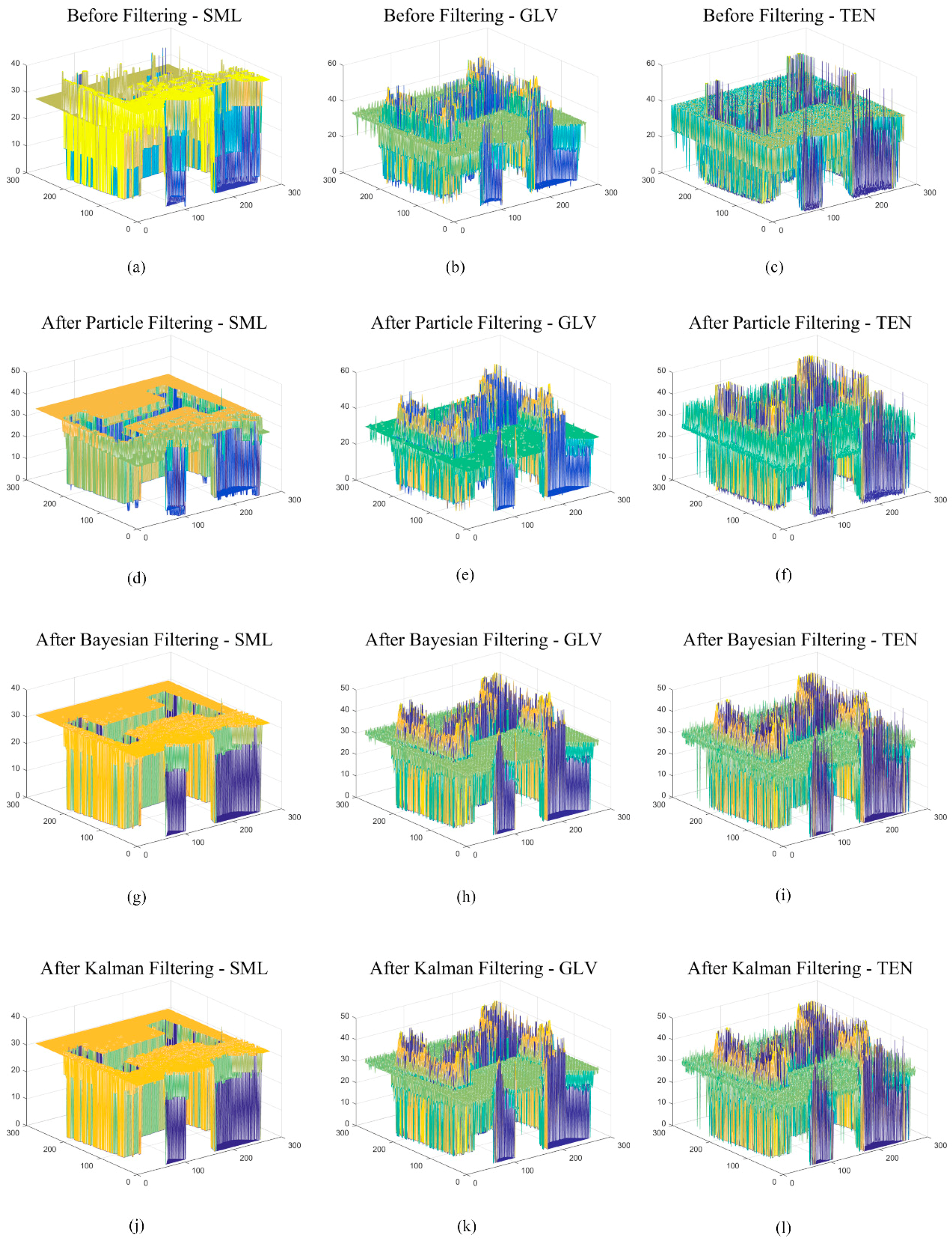
6.2. Experimental Results
7. Conclusions
Author Contributions
Funding
Acknowledgments
Conflicts of Interest
References
- Lin, J.; Ji, X.; Xu, W.; Dai, Q. Absolute Depth Estimation from a Single Defocused Image. IEEE Trans. Image Process. 2013, 22, 4545–4550. [Google Scholar] [PubMed]
- Humayun, J.; Malik, A.S. Real-time processing for shape-from-focus techniques. J. Real Time Image Process. 2016, 11, 49–62. [Google Scholar] [CrossRef]
- Lafarge, F.; Keriven, R.; Brédif, M.; Vu, H.H. A Hybrid Multiview Stereo Algorithm for Modeling Urban Scenes. IEEE Trans. Pattern Anal. Mach. Intell. 2013, 35, 5–17. [Google Scholar] [CrossRef] [PubMed]
- Ciaccio, E.J.; Tennyson, C.A.; Bhagat, G.; Lewis, S.K.; Green, P.H. Use of shape-from-shading to estimate three-dimensional architecture in the small intestinal lumen of celiac and control patients. Comput. Methods Programs Biomed. 2013, 111, 676–684. [Google Scholar] [CrossRef] [PubMed]
- Barron, J.T.; Malik, J. Shape, Illumination, and Reflectance from Shading. IEEE Trans. Pattern Anal. Mach. Intell. 2015, 37, 1670–1687. [Google Scholar] [CrossRef]
- De Vries, S.C.; Kappers, A.M.L.; Koenderink, J.J.; Vries, S.C. Shape from stereo: A systematic approach using quadratic surfaces. Percept. Psychophys. 1993, 53, 71–80. [Google Scholar] [CrossRef] [PubMed][Green Version]
- Super, B.J.; Bovik, A.C. Shape from Texture Using Local Spectral Moments. IEEE Trans. Pattern Anal. Mach. Intell. 1995, 17, 333–343. [Google Scholar] [CrossRef]
- Parashar, S.; Pizarro, D.; Bartoli, A. Isometric Non-Rigid Shape-From-Motion in Linear Time. In Proceedings of the IEEE Conference on Computer Vision and Pattern Recognition (CVPR), Las Vegas, NV, USA, 27–30 June 2016; pp. 4679–4687. [Google Scholar]
- Favaro, P.; Soatto, S.; Burger, M.; Osher, S.J. Shape from Defocus via Diffusion. IEEE Trans. Pattern Anal. Mach. Intell. 2008, 30, 518–531. [Google Scholar] [CrossRef] [PubMed]
- Tiantian, F.; Hongbin, Y. A novel shape from focus method based on 3D steerable filters for improved performance on treating textureless region. Opt. Commun. 2018, 410, 254–261. [Google Scholar]
- Nayar, S.K.; Nakagawa, Y. Shape from Focus. IEEE Trans. Pattern Anal. Mach. Intell. 1994, 16, 824–831. [Google Scholar] [CrossRef]
- Pertuz, S.; Puig, D.; García, M.A. Analysis of focus measure operators for shape-from-focus. Pattern Recognit. 2013, 46, 1415–1432. [Google Scholar] [CrossRef]
- Rusiñol, M.; Chazalon, J.; Ogier, J.M. Combining Focus Measure Operators to Predict OCR Accuracy in Mobile-Captured Document Images. In Proceedings of the 2014 11th IAPR International Workshop on Document Analysis Systems, Tours, France, 7–10 April 2014; pp. 181–185. [Google Scholar]
- Xie, H.; Rong, W.; Sun, L. Construction and evaluation of a wavelet-based focus measure for microscopy imaging. Microsc. Res. Tech. 2007, 70, 987–995. [Google Scholar] [CrossRef] [PubMed]
- Choi, T.S.; Malik, A.S. Vision and Shape—3D Recovery Using Focus; Sejong Publishing: Busan, Korea, 2008. [Google Scholar]
- Lee, I.-H.; Mahmood, M.T.; Choi, T.-S. Robust Focus Measure Operator Using Adaptive Log-Polar Mapping for Three-Dimensional Shape Recovery. Microsc. Microanal. 2015, 21, 442–458. [Google Scholar] [CrossRef] [PubMed]
- Asif, M.; Choi, T.-S. Shape from focus using multilayer feedforward neural networks. IEEE Trans. Image Process. 2001, 10, 1670–1675. [Google Scholar] [CrossRef] [PubMed]
- Mahmood, M.T.; Choi, T.-S.; Choi, W.-J.; Choi, W. PCA-based method for 3D shape recovery of microscopic objects from image focus using discrete cosine transform. Microsc. Res. Tech. 2008, 71, 897–907. [Google Scholar]
- Ahmad, M.; Choi, T.-S. A heuristic approach for finding best focused shape. IEEE Trans. Circuits Syst. Video Technol. 2005, 15, 566–574. [Google Scholar] [CrossRef]
- Muhammad, M.S.; Choi, T.S. A Novel Method for Shape from Focus in Microscopy using Bezier Surface Approximation. Microsc. Res. Tech. 2010, 73, 140–151. [Google Scholar] [CrossRef] [PubMed]
- Muhammad, M.; Choi, T.-S. Sampling for Shape from Focus in Optical Microscopy. IEEE Trans. Pattern Anal. Mach. Intell. 2012, 34, 564–573. [Google Scholar] [CrossRef]
- Lee, I.H.; Mahmood, M.T.; Shim, S.O.; Choi, T.S. Optimizing image focus for 3D shape recovery through genetic algorithm. Multimed. Tools Appl. 2014, 71, 247–262. [Google Scholar] [CrossRef]
- Malik, A.S.; Choi, T.-S. Consideration of illumination effects and optimization of window size for accurate calculation of depth map for 3D shape recovery. Pattern Recognit. 2007, 40, 154–170. [Google Scholar] [CrossRef]
- Malik, A.S.; Choi, T.-S. A novel algorithm for estimation of depth map using image focus for 3D shape recovery in the presence of noise. Pattern Recognit. 2008, 41, 2200–2225. [Google Scholar] [CrossRef]
- Jang, H.-S.; Muhammad, M.S.; Choi, T.-S. Removal of jitter noise in 3D shape recovery from image focus by using Kalman filter. Microsc. Res. Tech. 2017, 81, 207–213. [Google Scholar]
- Jang, H.-S.; Muhammad, M.S.; Choi, T.-S. Bayes Filter based Jitter Noise Removal in Shape Recovery from Image Focus. J. Imaging Sci. Technol. 2019, 63, 1–12. [Google Scholar] [CrossRef]
- Jang, H.-S.; Muhammad, M.S.; Choi, T.-S. Optimal depth estimation using modified Kalman filter in the presence of non-Gaussian jitter noise. Microsc. Res. Tech. 2018, 82, 224–231. [Google Scholar] [PubMed]
- Vasebi, A.; Bathaee, S.; Partovibakhsh, M. Predicting state of charge of lead-acid batteries for hybrid electric vehicles by extended Kalman filter. Energy Convers. Manag. 2008, 49, 75–82. [Google Scholar] [CrossRef]
- Frühwirth, R. Application of Kalman filtering to track and vertex fitting. Nucl. Instrum. Methods Phys. Res. A 1987, 262, 444–450. [Google Scholar] [CrossRef]
- Harvey, A.C. Applications of the Kalman Filter in Econometrics; Cambridge University Press: Cambridge, UK, 1987. [Google Scholar]
- Boulfelfel, D.; Rangayyan, R.; Hahn, L.; Kloiber, R.; Kuduvalli, G. Two-dimensional restoration of single photon emission computed tomography images using the Kalman filter. IEEE Trans. Med. Imaging 1994, 13, 102–109. [Google Scholar] [CrossRef] [PubMed]
- Bock, Y.; Crowell, B.W.; Webb, F.H.; Kedar, S.; Clayton, R.; Miyahara, B. Fusion of High-Rate GPS and Seismic Data: Applications to Early Warning Systems for Mitigation of Geological Hazards. In Proceedings of the American Geophysical Union Fall Meeting, San Francisco, CA, USA, 15–19 December 2008. [Google Scholar]
- Miall, R.C.; Wolpert, D. Forward Models for Physiological Motor Control. Neural Netw. 1996, 9, 1265–1279. [Google Scholar] [CrossRef]
- Frieden, B.R. Probability, Statistical Optics, and Data Testing; Springer: Berlin, Germany, 2001. [Google Scholar]
- Goodman, J.W. Speckle Phenomena in Optics; Roberts and Company Publishers: Englewood, CO, USA, 2007. [Google Scholar]
- Akselsen, B. Kalman Filter Recent Advances and Applications; Scitus Academics: New York, NY, USA, 2016. [Google Scholar]
- Pan, J.; Yang, X.; Cai, H.; Mu, B. Image noise smoothing using a modified Kalman filter. Neurocomputing 2016, 173, 1625–1629. [Google Scholar] [CrossRef]
- Ribeiro, M.I. Kalman and Extended Kalman Filters: Concept, Derivation and Properties; Institute for Systems and Robotics: Lisbon, Portugal, 2004. [Google Scholar]
- Welch, G.; Bishop, G. An Introduction to the Kalman Filter; University of North Carolina at Chapel Hill: Chapel Hill, NC, USA, 1995. [Google Scholar]
- Subbarao, M.; Lu, M.-C. Image sensing model and computer simulation for CCD camera systems. Mach. Vis. Appl. 1994, 7, 277–289. [Google Scholar]
- Tagade, P.; Hariharan, K.S.; Gambhire, P.; Kolake, S.M.; Song, T.; Oh, D.; Yeo, T.; Doo, S. Recursive Bayesian filtering framework for lithium-ion cell state estimation. J. Power Sources 2016, 306, 274–288. [Google Scholar] [CrossRef]
- Hajimolahoseini, H.; Amirfattahi, R.; Gazor, S.; Soltanian-Zadeh, H. Robust Estimation and Tracking of Pitch Period Using an Efficient Bayesian Filter. IEEE/ACM Trans. Audio Speech Lang. Process. 2016, 24, 1. [Google Scholar] [CrossRef]
- Li, T.; Corchado, J.M.; Bajo, J.; Sun, S.; De Paz, J.F. Effectiveness of Bayesian filters: An information fusion perspective. Inf. Sci. 2016, 329, 670–689. [Google Scholar] [CrossRef]
- Yang, T.; Laugesen, R.S.; Mehta, P.G.; Meyn, S.P. Multivariable feedback particle filter. Automatica 2016, 71, 10–23. [Google Scholar] [CrossRef]
- Zhou, H.; Deng, Z.; Xia, Y.; Fu, M. A new sampling method in particle filter based on Pearson correlation coefficient. Neurocomputing 2016, 216, 208–215. [Google Scholar] [CrossRef]
- Wang, D.; Yang, F.; Tsui, K.-L.; Zhou, Q.; Bae, S.J. Remaining Useful Life Prediction of Lithium-Ion Batteries Based on Spherical Cubature Particle Filter. IEEE Trans. Instrum. Meas. 2016, 65, 1282–1291. [Google Scholar] [CrossRef]
- Mahmood, M.T.; Majid, A.; Choi, T.-S. Optimal depth estimation by combining focus measures using genetic programming. Inf. Sci. 2011, 181, 1249–1263. [Google Scholar] [CrossRef]


| Notation | Description |
|---|---|
| Position of each image frame without jitter noise | |
| Standard deviation of jitter noise | |
| Best focused position through Gaussian approximation in each object point | |
| Standard deviation of Gaussian focus curve | |
| The amount of jitter noise before or after filtering | |
| Position of each image frame after Kalman filtering | |
| Position of each image frame before Kalman filtering | |
| Total number of iterations of filters |
| Focus Measure Operators | SML | GLV | TEN |
|---|---|---|---|
| Before Filtering | 9.2629 | 12.4038 | 15.2304 |
| After Particle Filtering | 9.1993 | 10.9459 | 11.2293 |
| After Bayesian Filtering | 7.3260 | 8.2659 | 8.4961 |
| After Kalman Filtering | 7.3169 | 8.1400 | 8.3652 |
| Focus Measure Operators | SML | GLV | TEN |
|---|---|---|---|
| Before Filtering | 0.7831 | 0.7430 | 0.7121 |
| After Particle Filtering | 0.7925 | 0.8157 | 0.7914 |
| After Bayesian Filtering | 0.9536 | 0.9427 | 0.9200 |
| After Kalman Filtering | 0.9541 | 0.9438 | 0.9206 |
| Focus Measure Operators | SML | GLV | TEN |
|---|---|---|---|
| Before Filtering | 20.1276 | 17.8644 | 16.0812 |
| After Particle Filtering | 20.4604 | 18.9504 | 18.7284 |
| After Bayesian Filtering | 22.3481 | 21.3897 | 21.1510 |
| After Kalman Filtering | 22.3588 | 21.5229 | 21.2859 |
| Focus Measure Operators | SML | GLV | TEN |
|---|---|---|---|
| Before Filtering | 21.6257 | 19.5639 | 19.1356 |
| After Particle Filtering | 18.2074 | 18.1522 | 18.3674 |
| After Bayesian Filtering | 16.9866 | 17.4630 | 17.9747 |
| After Kalman Filtering | 16.9458 | 17.4064 | 17.9344 |
| Focus Measure Operators | SML | GLV | TEN |
|---|---|---|---|
| Before Filtering | 0.8133 | 0.8661 | 0.8570 |
| After Particle Filtering | 0.8941 | 0.9083 | 0.8873 |
| After Bayesian Filtering | 0.9518 | 0.9496 | 0.9316 |
| After Kalman Filtering | 0.9527 | 0.9504 | 0.9325 |
| Focus Measure Operators | SML | GLV | TEN |
|---|---|---|---|
| Before Filtering | 12.2884 | 13.3517 | 13.3074 |
| After Particle Filtering | 13.2806 | 13.8092 | 13.5967 |
| After Bayesian Filtering | 14.0878 | 13.8476 | 13.6162 |
| After Kalman Filtering | 14.1087 | 13.8758 | 13.6389 |
| Experimented Objects | Particle Filter | Bayes Filter | Kalman Filter |
|---|---|---|---|
| Simulated cone | 0.651821 | 0.112929 | 0.006780 |
| Coin | 0.699162 | 0.125152 | 0.009283 |
| LCD-TFT filter | 0.624884 | 0.112957 | 0.007769 |
| Letter-I | 0.688404 | 0.112758 | 0.007259 |
| Experimented Objects | Particle Filter | Bayes Filter | Kalman Filter |
|---|---|---|---|
| Simulated cone | 0.637766 | 0.113022 | 0.008112 |
| Coin | 0.677874 | 0.124471 | 0.009683 |
| LCD-TFT filter | 0.625544 | 0.116263 | 0.007738 |
| Letter-I | 0.636709 | 0.112466 | 0.009179 |
© 2019 by the authors. Licensee MDPI, Basel, Switzerland. This article is an open access article distributed under the terms and conditions of the Creative Commons Attribution (CC BY) license (http://creativecommons.org/licenses/by/4.0/).
Share and Cite
Jang, H.-S.; Muhammad, M.S.; Yun, G.; Kim, D.H. Sampling Based on Kalman Filter for Shape from Focus in the Presence of Noise. Appl. Sci. 2019, 9, 3276. https://doi.org/10.3390/app9163276
Jang H-S, Muhammad MS, Yun G, Kim DH. Sampling Based on Kalman Filter for Shape from Focus in the Presence of Noise. Applied Sciences. 2019; 9(16):3276. https://doi.org/10.3390/app9163276
Chicago/Turabian StyleJang, Hoon-Seok, Mannan Saeed Muhammad, Guhnoo Yun, and Dong Hwan Kim. 2019. "Sampling Based on Kalman Filter for Shape from Focus in the Presence of Noise" Applied Sciences 9, no. 16: 3276. https://doi.org/10.3390/app9163276
APA StyleJang, H.-S., Muhammad, M. S., Yun, G., & Kim, D. H. (2019). Sampling Based on Kalman Filter for Shape from Focus in the Presence of Noise. Applied Sciences, 9(16), 3276. https://doi.org/10.3390/app9163276