Multi-Scale Heterogeneous 3D CNN for False-Positive Reduction in Pulmonary Nodule Detection, Based on Chest CT Images

Abstract

Currently, lung cancer has one of the highest mortality rates because it is often caught too late. Therefore, early detection is essential to reduce the risk of death. Pulmonary nodules are considered key indicators of primary lung cancer. Developing an efficient and accurate computer-aided diagnosis system for pulmonary nodule detection is an important goal. Typically, a computer-aided diagnosis system for pulmonary nodule detection consists of two parts: candidate nodule extraction and false-positive reduction of candidate nodules. The reduction of false positives (FPs) of candidate nodules remains an important challenge due to morphological characteristics of nodule height changes and similar characteristics to other organs. In this study, we propose a novel multi-scale heterogeneous three-dimensional (3D) convolutional neural network (MSH-CNN) based on chest computed tomography (CT) images. There are three main strategies of the design: (1) using multi-scale 3D nodule blocks with different levels of contextual information as inputs; (2) using two different branches of 3D CNN to extract the expression features; (3) using a set of weights which are determined by back propagation to fuse the expression features produced by step 2. In order to test the performance of the algorithm, we trained and tested on the Lung Nodule Analysis 2016 (LUNA16) dataset, achieving an average competitive performance metric (CPM) score of 0.874 and a sensitivity of 91.7% at two FPs/scan. Moreover, our framework is universal and can be easily extended to other candidate false-positive reduction tasks in 3D object detection, as well as 3D object classification.

1. Introduction

Lung cancer is one of the deadliest diseases with one of the highest mortality rates in the world [1]. Early asymptomatic manifestations of lung cancer may lead patients to miss the optimal treatment time; thus, early detection and treatments are essential to reduce the risk of death. Pulmonary nodules are considered key indicators of primary lung cancer [2]. The National Lung Screening Trial (NLST) [3] test shows that using low-dose chest computed tomography (CT) to examine pulmonary nodules in high-risk populations can reduce lung cancer mortality by 20%. Therefore, the detection of pulmonary nodules is very important for the early detection of lung cancer. Pulmonary nodules have many clinical manifestations, but one of the most prevalent is when nodules are irregular circles with a diameter of 3 mm to 30 mm [4]. According to pathological knowledge, a computer-aided diagnosis system for pulmonary nodule detection can be developed to reduce the workload of doctors, reduce misdiagnosis rate, and improve the efficiency of diagnosis.

Typically, a computer-aided diagnosis system (CAD) for pulmonary nodule detection consists of two parts: (1) candidate nodule detection, and (2) false-positive (FP) reduction of candidate nodules. In the candidate nodule detection step, the system detects as many candidates as possible to ensure high sensitivity without considering specificity. This is accompanied by a large number of false-positive nodules detected [5]. To reduce false positives, the system classifies the real nodules and non-nodules in the set of candidates detected in the previous step to reduce the number of false positives. False-positive reduction of candidate nodules is the most important part of a computer-aided diagnosis system for pulmonary nodule detection [6]. As far as we know, the current computer-aided diagnosis system (CAD) for pulmonary nodule detection is still in the development stage. Although the CAD system can improve the reading efficiency of radiologists, it is still not well used in clinical applications. Therefore, it is important to develop an advanced algorithm with high performance.

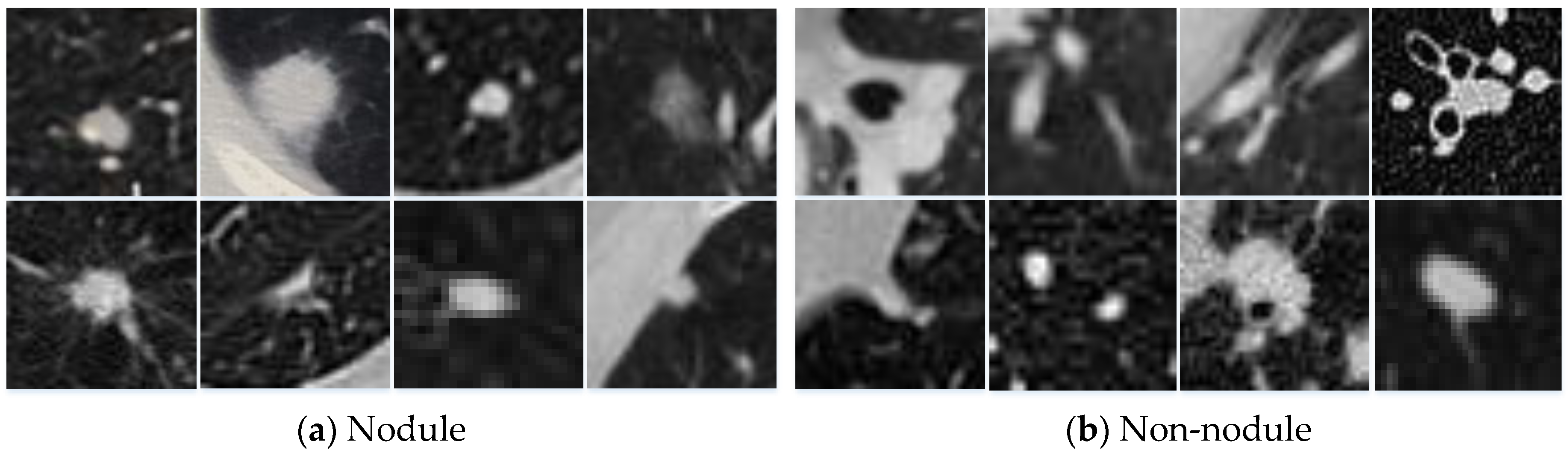
Pathologically, there are many types of nodules (e.g., ground glass nodules, solitary nodules, etc.) [7]. Various nodules have complex morphologies and multiple structures, and they often adhere to the trachea, blood vessels, and other organs. The morphological features of the candidate nodules are often similar to organs in the thoracic cavity (e.g., lymph nodes, blood vessels, etc.). This greatly increases the difficulty of reducing false positives in candidate nodules. Figure 1 shows an example of different types of nodules. This is why many researchers devoted their time to developing stable and effective algorithms to distinguish between nodules and non-nodules, thereby reducing false positives [8,9,10].

Recently, with the rapid development of deep learning techniques for medical image analysis [11,12,13,14,15], more and more researchers successfully applied convolutional neural networks (CNNs) to the detection of pulmonary nodules based on chest CT images [5,8,10,16,17,18], and achieved desirable results. By studying these methods, we can list three findings.

Firstly, the system that uses volumetric information has fewer false positives than methods that use two-dimensional (2D) slice information alone [5,16,17]. For example, Setio et al. [5] proposed a 2D multi-view CNN, which classified nodules based on slices from nine different views. Although the method utilized multiple views of the pulmonary nodules, to some extent, the three-dimensional (3D) information of the nodules was still not fully utilized. Therefore, Ding et al. [17] proposed to use a 3D nodule block as input for 3D-CNN, which was effective in reducing false positives.

Secondly, using multi-scale information of nodules can improve the performance of the algorithm [8,10,18]. For example, Kim et al. [8] proposed a multi-scale gradual integration CNN, which fused three scales of nodules gradually according to two different rules. This method used the 3D nodule information as a channel and used a 2D convolution kernel.

Thirdly, network parallel connections can improve false-positive performance. Dou et al. [10] proposed a multi-scale parallel 3D-CNN, which extracted blocks of three different scales for each candidate nodule. The classification calculations were made for each nodule block separately; then, the three classification results were combined according to a set of weights. The weights were determined manually, not trained from the dataset.

In this paper, we propose a multi-scale heterogeneous 3D CNN (MSH-CNN) for false-positive reduction of pulmonary nodules, which differs from other methods mainly in (1) using the 3D method. By making full use of 3D spatial information, our network can learn representative features with higher discernment than that of 2D CNN. (2) In order to cope with the large variations of nodules and more clearly distinguish them from other similar organizations, we use multi-scale blocks of the nodule as input. According to the characteristics of the nodule and organs surrounding the nodule, a novel heterogeneous network was designed to extract the expressions features. (3) We use a set of weights which are determined by back propagation to fuse the expression features. The experimental performance on the Lung Nodule Analysis 2016 (LUNA16) dataset demonstrates the effectiveness of our method and shows a brighter prospect on large datasets.

Our main contributions are as follows:

(1) We propose a novel 3D CNN for false-positive reduction of pulmonary nodules.

(2) We evaluate the effect of multi-scale heterogeneous 3D CNN with different structures on the reduction of false-positive nodules.

(3) Our method is tested on the Lung Nodule Analysis 2016 (LUNA16) [19] dataset, and the measure of performance surpasses most documented methods.

The rest of this paper is organized as follows: Section 2 introduces the existing methods in the literature. Section 3 describes our method. We introduce the algorithm performance comparison method and evaluate the impact of different structures on the results in Section 4. In Section 5, we discuss the reasons for the effectiveness of our method and the future directions for improvement. The conclusions are drawn in Section 6.

2. Related Work

In early tumor imaging research, researchers mainly focused on using traditional computer vision methods to artificially design expression features according to the appearance of nodules. For example, Messay et al. [20] designed an algorithm for segmentally identifying nodules based on the shape, position, brightness, and gradient characteristics of candidate nodules. Jacobs et al. [21] extracted 128 features based on shape, brightness, texture, and neighboring organ information of the nodule. The method used six classifiers to test and compared the results: support vector machine using radial basis function kernel (SVM-RBF), k-nearest neighbor, GentleBoost, random forest, recent mean, and linear classifiers. The sensitivity of the GentleBoost classifier reached 80% at 1.0 FP/scan. Although this method achieved good results, only pulmonary nodules with certain characteristics (e.g., shape, size, and texture) were found. However, these surface features lacked discrimination because the shape, size, and texture of pulmonary nodules vary widely, making it difficult to distinguish between real nodules and false-positive nodules.

Recently, deep neural networks became more common than manual design features. By studying deep neural network applications to reduce false-positive pulmonary nodules, we can find characteristic patterns. The use of 3D volumetric information, multi-scale nodule block input, and multi-branch network parallelization became more and more popular, and achieved better and better results.

In using 3D volumetric information, researchers gradually shifted away from using multi-view slice information of nodules to volumetric information of nodules. For example, Roth et al. [16] proposed the concept called 2.5D, which extracted three orthogonal slices for each candidate nodule, and used convolutional neural networks to extract expression features for classification. Setio et al. [5] proposed a 2D multi-view convolutional neural network that extracted nine slices of different views for each nodule, inputting them into convolutional neural networks to extract expression features, and finally merging these features by certain methods. In the LIDC-IDRI [22] dataset test, this method achieved good sensitivity, but still had some defects when the false-positive rate was low. Therefore, Ding et al. [17] proposed to extract 3D nodule blocks as the input of 3D-CNN according to the location of candidate nodules.

In the multi-scale nodule block inputting process, Shen et al. [18] proposed a multi-scale CNN, i.e., MCNN, to extract blocks (of different scales) according to candidate nodule coordinates. All the blocks were merged and a convolutional neural network was used to extract expression features for classification. Kim et al. [8] proposed multi-scale gradual integration CNN, using 2D convolution kernels to gradually fuse nodule blocks of different scales, and two branches were input to extract expression features. Finally, the nodules were classified by fusing these expression features. Multi-scale blocks have several advantages over single blocks; the advantages are as follows: (1) multi-scale blocks can completely segment nodules with large diameters; (2) multi-scale blocks can ensure the smaller-diameter nodules maintain a larger proportion of the block; (3) multi-scale blocks can increase the neighboring organ information of the nodule and bring abundant volumetric information while ensuring the integrity of nodule information.

In multi-branch network parallelization, Dou et al. [10] extracted nodule blocks of three scales and input them into three parallel branches for classification. Finally, the classification results were fused by the weights determined manually. When Kim et al. [8] fused the two parallel branches, a simple addition method was used to fuse them. Compared to a single branch network, multi-branch networks can extract more abundant complementary expression features. These complementary expression features can significantly improve the performance of the network after fusion.

3. Method

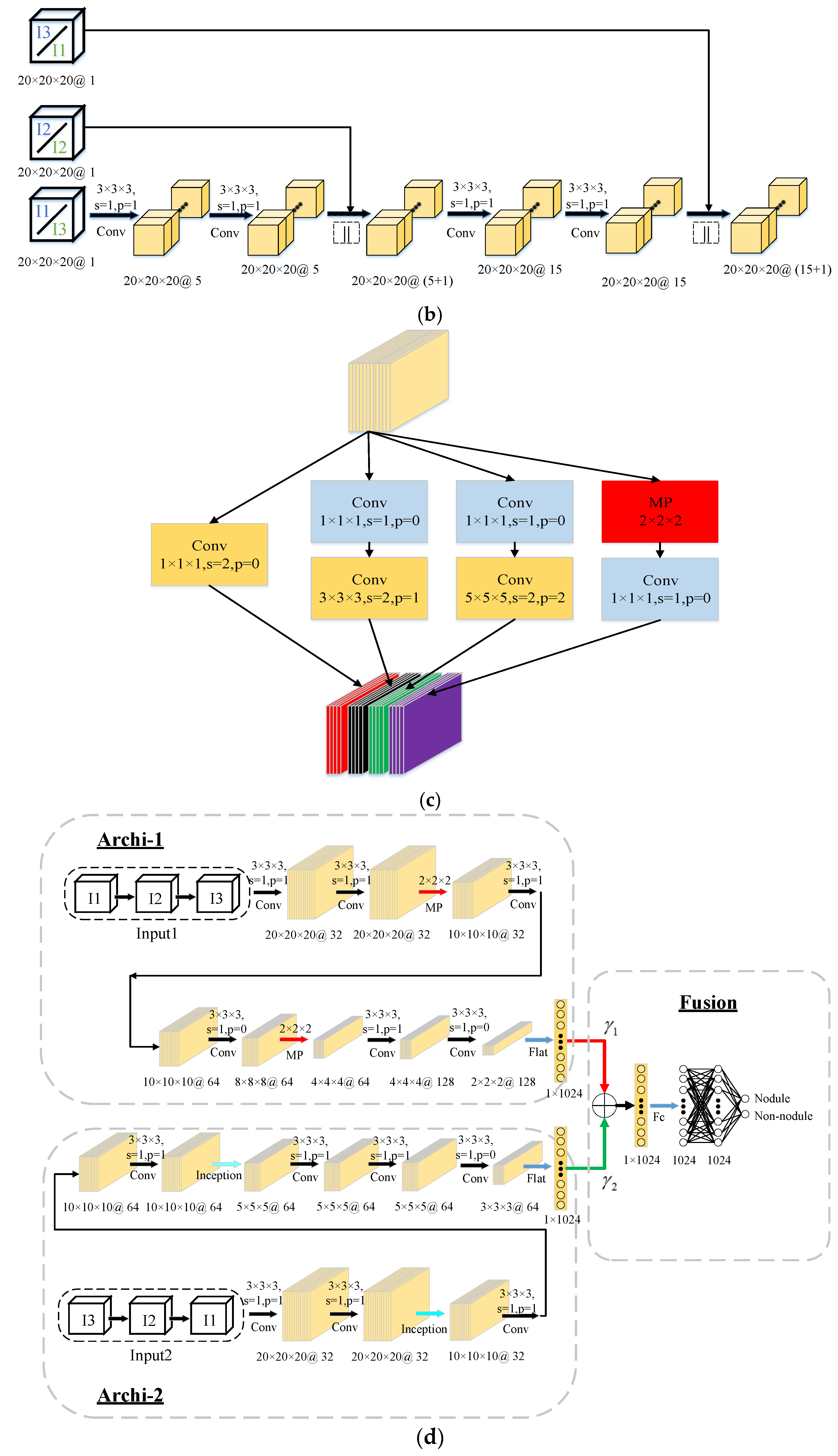
Our proposed multi-scale heterogeneous 3D CNN framework for false-positive reduction in pulmonary nodule detection shown in Figure 2d consists of three main parts: 3D multi-scale gradual integration, heterogeneous feature extraction, and automatic learning weight fusion. Inspired by Reference [8], for each candidate nodule, we used the coordinates of the center of the nodule to extract nodule blocks of three different scales. The three scales were $40\times 40\times 40$, $30\times 30\times 30$, and $20\times 20\times 20$, and we resized the three scales to transform them into $20\times 20\times 20$ blocks, which are represented as I1, I2, and I3 (Figure 2a).

3.1. 3D Multi-Scale Gradual Integration

When humans observe objects, they can retrieve meaningful information by changing the size of the field of view. Inspired by this concept, multi-scale nodule information is effective for false-positive reduction. We propose a 3D multi-scale gradual integration module in Figure 2b that uses 3D convolution kernels to gradually integrate nodule blocks of different scales. There are two fusion sequences, i.e., I1-I2-I3 (“Input1”) and I3-I2-I1 (“Input2”).

For the I1-I2-I3 (“Input1”) fusion order, the nodule block I1 firstly obtains the feature map F1 via two 3D convolution operations; then, the feature maps F1 and nodule blocks I2 are fused according to channel (shown by the symbol “||”) to obtain F1||I2. After each 3D convolution, the non-linear function ReLU is used as the activation function. The output of ReLU is computed via a batch norm. To ensure that the feature map F1 and the nodule block I2 can be fused according to the channel, we use zero padding to ensure F1 and I2 are equivalent sizes. After combining the channels, F1||I2 also uses two 3D convolution operations to obtain the feature map F12; then, F12 and I3 are fused according to channel (shown by the symbol “||”) to obtain F12||I3, i.e., Input 1. For the fusion order of I3-I2-I1, the same calculation is used, except that the input order of the nodule blocks is reversed.

Therefore, nodule block I1 is resized and contains the most information about neighboring organs of the nodule, and I3 contains the least information about neighboring organs. For the I1-I2-I3 case, the input nodules contain less and less information of neighboring organs, mainly to enable the network to gradually focus on the morphological characteristics of the nodules themselves. In contrast, for the I3-I2-I1 case, the input nodule blocks contain more and more information about the neighboring organs. Their main purpose is to let the network gradually pay more and more attention to the morphological characteristics of the neighboring nodule organs. For every two sequences, the network focuses on the morphological features of the nodule and its neighboring organs. Using a 3D convolution kernel, the system is able to more fully extract volume information of the nodules and their neighboring organs. It is worth noting that the multi-scale inputs are computed on the fly during training/testing.

3.2. Heterogeneous Feature Extraction

Considering the important influence of the receptive field and network structure on the classification performance, we input I1-I2-I3 (“Input 1”) and I3-I2-I1 (“Input 2”) into two branches of different structures (as shown in Figure 2d). In theory, the receptive field of the convolutional neural network changes with the network structure. If the receptive field is too small, the network is limited by local information and lacks the ability to discriminate between targets with great variation. If the receptive field is too large, too much redundant information and noise interfere with the training process and reduce the performance of the model. Therefore, different convolutional neural network structures are used for different scale inputs.

I1-I2-I3 (“Input1”) and I3-I2-I1 (“Input2”) gradually integrate the nodule blocks in different order and they mainly focus on different aspects (features). Therefore, by using two branches with different structures, the characteristics of “Input1” and “Input2” can be fully utilized to extract complementary expression features.

The branch structure of input “Input 1” is mainly composed of 3D convolution layers and 3D max-pooling layers. After each 3D convolution, ReLU is used as the activation function and batch norm is used for the output of ReLU.

The branch structure of “Input 2” is mainly composed of 3D convolution layers and 3D inception layers. Similar to the previous branches, after each 3D convolution and 3D inception, ReLU is used as the activation function and batch norm is used for the output of ReLU. A detailed structure of the 3D inception step is shown in Figure 2c.

3.3. Automatic Learning Weight Fusion

In this part, we use a set of weights which are automatically determined by back propagation to fuse the expression features extracted from the two branches, as shown in Figure 2d. The weights ${\gamma }_1$ and ${\gamma }_2$ are determined by the Adam optimizer [23] and back propagation, which is the same way in which the parameters w and b in the convolution kernel are updated. The formula is as follows:

$$\{\begin{array}{c}{m}_t={\beta }_1·m_{t-1}+\left(1-{\beta }_1\right)·\frac{\partial L{\left(w,b,\gamma \right)}_{t-1}}{\partial {\gamma }_{t-1}}\\ v_t={\beta }_2·v_{t-1}+\left(1-{\beta }_2\right)·{\left(\frac{\partial L{\left(w,b,\gamma \right)}_{t-1}}{\partial {\gamma }_{t-1}}\right)}^2\\ \widehat{m_t}=m_t/\left(1-{\beta }_1^t\right)\\ \widehat{v_t}=v_t/\left(1-{\beta }_2^t\right)\\ {\gamma }_t={\gamma }_{t-1}-\alpha ·\widehat{m_t}/\left(\sqrt{\widehat{v_t}}+\epsilon \right)\end{array},$$

(1)

where ${\beta }_1$ and ${\beta }_2$ are parameters in the Adam optimizer, commonly represented by 0.9 and 0.999, $\mathrm{L}\left(\mathrm{w},\mathrm{b},\mathsf{\gamma }\right)$ is the loss function, and $\alpha$ is the learning rate. The initial values of $m_t$ and $v_t$ are both 0. The $\epsilon$ is a small value, commonly set to ${10}^{-8}$.

For each candidate nodule $Li$, both branch networks can extract the expression features. We fuse the expression features after the flat layer and before the full connection layer. $E_1\left(Li\right)$ represents feature vectors of the branch 1 output (similar to branch 2). The feature vectors $E_{fusion}\left(Li\right)$ are fused by automatic learning weights as follows:

$$E_{fusion}\left(Li\right)={\gamma }_1{E}_1\left(Li\right)+{\gamma }_2{E}_2\left(Li\right),$$

(2)

where ${\gamma }_1$ and ${\gamma }_2$ are weights which are automatically determined by back propagation from the training process. The feature vectors $E_{fusion}\left(Li\right)$ can get the probability that $Li$ is a real nodule through the full connection layer and the softmax. In the fully connected layer, except for the final output layer, the middle layer uses ReLU as the activation function and uses dropout with a threshold of 0.5.

4. Experiments and Results

4.1. Dataset

We used the LUNA16 challenge dataset to evaluate the performance of the network. The LUNA16 dataset was derived from a larger public dataset, the Lung Image Database Consortium and Image Database Resource Initiative (LIDC-IDRI) [22]. The LUNA16 dataset is an LIDC-IDRI dataset that removes CT images of slice thicknesses greater than 3 mm, as well as those with space inconsistencies, and missing partial slices, resulting in 888 CT images. It contains 1186 real nodules, where each nodule is an irregular circle with a diameter of more than 3 mm, and most of them are located in the lung parenchyma central, with a few in the lung parenchyma periphery. The transverse plane size of each CT sample is $512\times 512$.

For false-positive reduction of pulmonary nodules, the LUNA16 challenge data provide two versions (V1 and V2) of the datasets. Each dataset contains the central coordinates of candidate nodules, the classification labels, and the corresponding patient identifier (ID). The dataset V1 was detected by three existing candidate detection algorithms [21,24,25] and contains 551,065 candidate nodules. The dataset was separated into nodule and non-nodule groups, where 1351 were labeled as nodules and 549,714 were labeled as non-nodules. Out of the 1186 real nodules previously recognized, 1120 of the 1351 labeled nodules are real nodules, and 231 are non-nodules. The dataset V2 contains 754,975 candidate nodules obtained by References [21,24,25,26,27], where 1557 were labeled as nodules, and 1166 are matched with the 1186 real nodules.

Table 1. Statistics of the dataset in the Lung Nodule Analysis 2016 (LUNA16) challenge. The number in parentheses indicates the number of nodule-labeled matches with 1186 real nodules. V—version.

Dataset	Candidates
	Nodule	Non-Nodule
V1	1351 (1120)	549,714
V2	1557 (1166)	753,418

summarizes the candidate nodule statistics of the dataset in the LUNA16 challenge.

4.2. Evaluations Metrics

We used the competitive performance metric (CPM) [28] score for the evaluation of the algorithm, which is a metric used in the LUNA16 challenge list. The score calculates average sensitivity at seven predefined false positives per scan (FP/scan) indices, i.e., 0.125, 0.25, 0.5, 1, 2, 4, and 8, on a free receiver operation characteristic (FROC) curve. Currently, an FP/scan is widely used in clinical practice in the range of 1 to 4.

4.3. Experimental Settings

In this paper, we used a Pytorch, Intel(R) Xeon(R) E5-2680 v4 central processing unit (CPU) with 2.4 GHz and an NVIDIA GeForce GTX 1080ti graphics processing unit (GPU) as the experimental platform. The learning rate was set to 0.003 and the batch size was set to 128. We applied the batch norm technique at the output of each convolutional layer, and, in order to avoid overfitting, L2 regularization was applied; we also used a dropout technique with a threshold of 0.5 at the fully connected layer. The optimizer chosen was Adam, and ${\beta }_1$ and ${\beta }_2$ were set at respectively 0.9 and 0.999. The loss function used was cross-entropy. The formula for cross entropy is as follows:

$$L=-\left[y\log \widehat{y}+\left(1-y\right)\log \left(1-\widehat{y}\right)\right],$$

(3)

where $y$ is labeled with 1 or 0 (i.e., 1 denotes nodule and 0 denotes non-nodule), and $\widehat{y}$ indicates the probability that the model predicts real nodules.

In the data preprocessing stage, we extracted $40\times 40\times 40$, $30\times 30\times 30$, and $20\times 20\times 20$ blocks for each sample via the central coordinates of the candidate nodules and used the nearest neighbor interpolation to transform them all into blocks. We used minimum–maximum normalization to ensure the algorithm converged faster by adjusting the data distribution of the sample. The intensities of the blocks were cut to [−1000, 400] Hounsfield units (HU)² and normalized to [0, 1].

We used a five-fold cross-validation method to evaluate the algorithm, randomly dividing the CT scans into five parts based on patients, such that four parts were used for training and one was used for testing. To deal with the class imbalance between nodules and non-nodules and to avoid overfitting, we used data augmentation for nodule samples. Specifically, we rotated the nodules by 90°, 180°, and 270° on a transverse plane and shifted the center along each axis by 1, 2 pixels; we also added Gaussian noise with a mean of 0 and variance of 0.4 to those added data. The number of nodules and non-nodules in the five-fold cross-validation is shown in

Table 2. Statistics of the dataset used for five-fold cross-validation.

Dataset		Fold 1		Fold 2		Fold 3		Fold 4		Fold 5
		Training	Test	Training	Test	Training	Test	Training	Test	Training	Test
V1	Patient	533	133	533	133	533	133	533	133	532	134
	Nodule	936	184	867	253	910	210	912	208	855	265
	Augmentation	101,088	-	93,636	-	191,916	-	98,496	-	92,340	-
	Non-nodule	439,022	110,692	440,811	108,903	438,087	111,627	444,860	104,854	436,076	113,638
V2	Patient	711	177	711	177	710	178	710	178	710	178
	Nodule	970	196	953	213	917	249	930	236	894	272
	Augmentation	100,440	-	102,924	-	99,036	-	104,760	-	96,552	-
	Non-nodule	598,891	154,527	602,299	151,119	605,820	147,598	606,027	147,391	600,635	152,783

.

4.4. Experimental Results

We used several models from References [5,8,10,29] as baselines. Dou et al. [10] was based on a 3D method, where they used three sizes of nodule blocks as inputs. UACNN [10] selected three slices of the candidate nodule center, 3 mm above and 3 mm below, as inputs. Setio et al. [5] extracted nine different views of the nodules as input based on a 2D method. Sakamoto et al. [29] eliminated prediction inconsistencies by raising the threshold at each iteration. Kim et al. [8] gradually integrated nodule blocks of three sizes as inputs, based on 2D convolution kernels.

Table 3. Competitive performance metric (CPM) scores of different methods on V1 dataset of LUNA16. FP—false positive; MSH-CNN—multi-scale heterogeneous three-dimensional (3D) convolutional neural network.

	FP/Scan	0.125	0.25	0.5	1	2	4	8	Average CPM
Sensitivity
V1	Dou et al. [10]	0.678	0.738	0.816	0.848	0.879	0.907	0.922	0.827
	UACNN [10]	0.655	0.745	0.807	0.849	0.880	0.907	0.925	0.824
	Setio et al. [5]	0.692	0.771	0.809	0.863	0.895	0.914	0.923	0.838
	Sakamoto et al. [29]	0.760	0.794	0.833	0.860	0.876	0.893	0.906	0.846
	Kim et al. [8]	0.880	0.894	0.907	0.912	0.914	0.919	0.927	0.908
	MSH-CNN (ours)	0.759	0.812	0.859	0.901	0.917	0.928	0.943	0.874

and

Table 4. CPM scores of different methods on V2 dataset of LUNA16.

	FP/Scan	0.125	0.25	0.5	1	2	4	8	Average CPM
Sensitivity
V2	Setio et al. [5]	0.669	0.760	0.831	0.892	0.923	0.944	0.960	0.854
	Kim et al. [8]	0.904	0.931	0.943	0.947	0.952	0.956	0.962	0.942
	MSH-CNN (ours)	0.833	0.867	0.932	0.953	0.960	0.977	0.984	0.929

summarize the CPM scores of these different methods on V1 and V2 datasets.

Table 3 summarizes the best performance of our MSH-CNN algorithm on the V1 dataset. The proposed MSH-CNN was superior to most methods in terms of average CPM. Compared to Dou et al. [10], UACNN, and Setio et al. [5] in terms of average CPM, our 3D network had increases by 0.047, 0.050, and 0.036, respectively. Our method was 0.001 lower than Sakamoto’s method [29] at the 0.125 FP/scan, but it had a higher average CPM and sensitivity at the 0.25, 0.5, 1, 2, 4, and 8 FP/scan. In comparison with Kim et al. [8], although the sensitivity of our method was lower when the FP/scan was less than 1, our network still achieved the best performance at the 2, 4, and 8 FP/scan. Our method outperformed most methods in the false-positive rates of range 1–4 which are commonly used in clinical applications [30]. 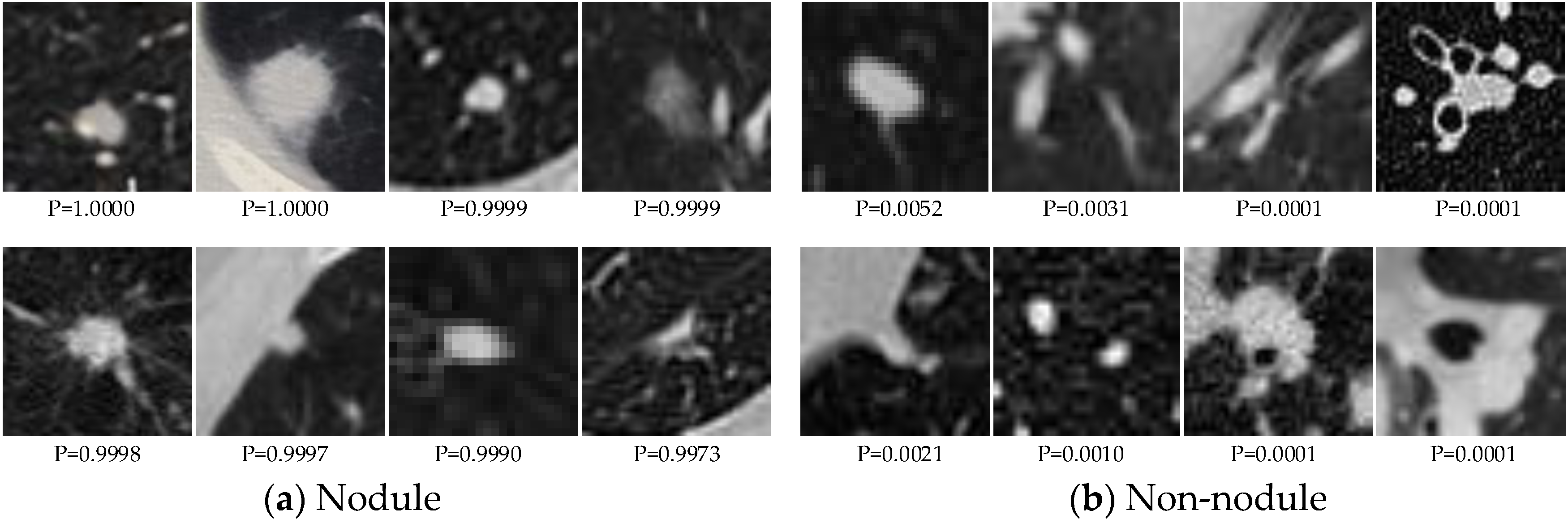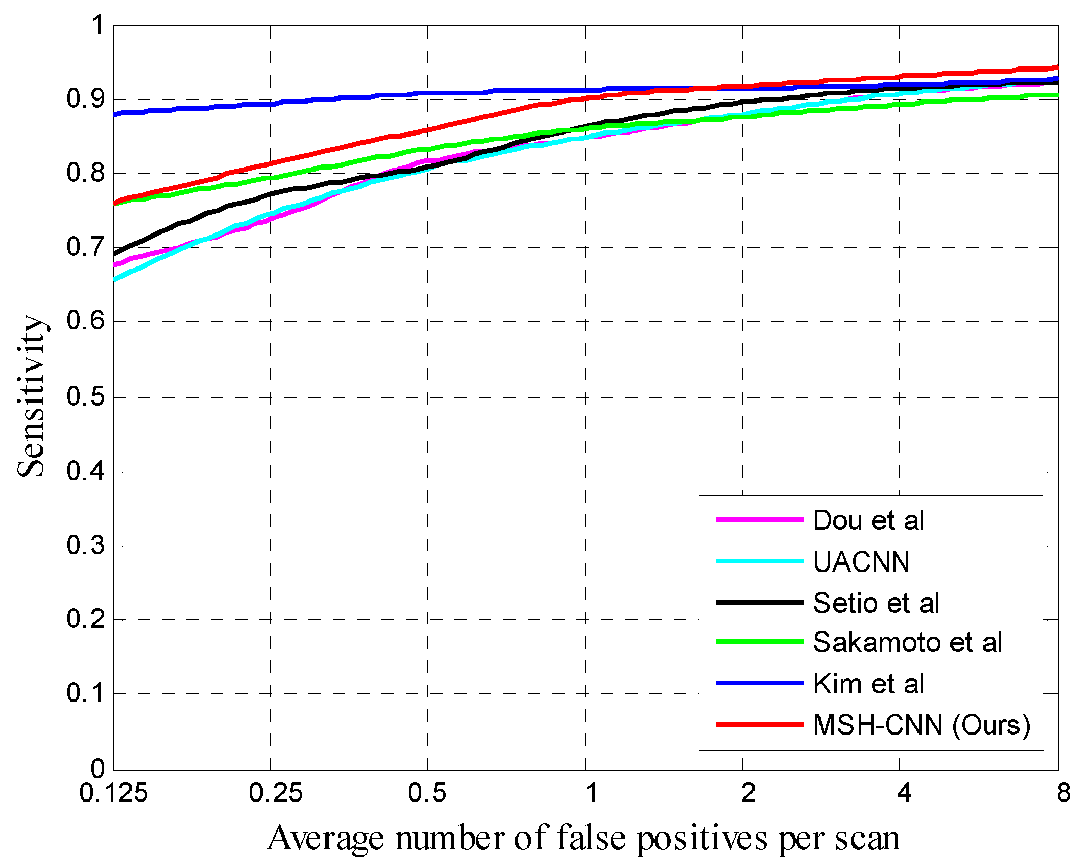Figure 3 shows some examples of correctly classified candidate nodules. The FROC curves of different methods are shown in Figure 4.

We also tested performance on the large-sized V2 dataset as presented in Table 4. The proposed 3D method was better than other methods at high FP/scan. Specifically, the average CPM scores of our method and the sensitivity at different FP/scan were higher than those of Setio et al. [5]. In comparison with Kim et al. [8], the sensitivity of our network at 0.125, 0.25, and 0.5 FP/scan was lower, but it still achieved the best performance at the 1, 2, 4 and 8 FP/scan. It is worth noting that, comparing the performance of various algorithms on the V1 and V2 datasets, we can see that our sensitivity was higher than that of Kim et al. [8] in the false-positive rates of range 1–4 which are commonly used in clinical applications [30], and, as the dataset increased, our 3D method performed better and better at low FP/scan, even exceeding that of Kim et al. [8] at the 1 FP/scan. In terms of average CPM, Setio et al. [5], Kim et al. [8], and our method increased by 0.016, 0.034, and 0.055, respectively, and our 3D network had the best improvement.

4.5. Effects of the Proposed Methods

In order to quantitatively analyze our proposed MSH-CNN method, we designed the following CNNs for comparison:

(1) MSH-CNN-RI: The 3D multi-scale gradual integration module (I1-I2-I3 and I3-I2-I1) in MSH-CNN was replaced with the radical integration I1||I2||I3 in the same layer. The “||” symbol indicates concatenation by channel, as shown in Figure 5.

(2) MSH-CNN-IC: I1-I2-I3 (“Input 1”) and I3-I2-I1 (“Input 2”) in the MSH-CNN were interchanged, and Input 1 was input into Archi-2, while Input 2 was input into Archi-1, and the structure was similar to that shown in Figure 2d.

(3) MSH-CNN-AF: The fusion method of the MSH-CNN was modified to addition fusion without weights.

(4) MSH-CNN-II: In MSH-CNN, the network in Archi-1 was replaced by that in Archi-2 (including 3D inception), so that both branches contained 3D inception.

(5) MSH-CNN-EI: In MSH-CNN, the network in Archi-2 was replaced by that in Archi-1 (excluding 3D inception), so that neither branch contained 3D inception.

(6) MSH-CNN-LT: The training and test sets were expanded, and the MSH-CNN model was trained and tested on the datasets of LUNA16 + Tianchi. The Tianchi dataset was provided by the Aliabad Cloud of Intelligent Diagnosis of Pulmonary Nodules. The training and validation sets contained a total of 800 CT samples and 1245 nodules.

Table 5. CPM scores of different structure networks. MSH-CNN-RI radically integrates nodule blocks; MSH-CNN-IC interchange the inputs of two branches; MSH-CNN-AF uses addition fusion without weights; MSH-CNN-II has both branches containing inception; MSH-CNN-EI has neither branch containing Inception; MSH-CNN-LT uses the LUNA16 + Tianchi dataset.

	FP/Scan	0.125	0.25	0.5	1	2	4	8	Average CPM
Sensitivity
MSH-CNN-RI		0.716	0.773	0.831	0.885	0.900	0.904	0.936	0.849
MSH-CNN-IC		0.763	0.811	0.840	0.905	0.909	0.926	0.942	0.871
MSH-CNN-AF		0.744	0.782	0.842	0.873	0.897	0.915	0.940	0.856
MSH-CNN-II		0.771	0.818	0.839	0.885	0.905	0.917	0.938	0.868
MSH-CNN-EI		0.741	0.776	0.835	0.870	0.913	0.920	0.943	0.857
MSH-CNN (ours)		0.759	0.812	0.859	0.901	0.917	0.928	0.943	0.874
MSH-CNN-LT		0.932	0.944	0.957	0.976	0.982	0.989	0.991	0.967

summarizes the best performance of each network. Our method had higher average CPM score than other networks, which can be seen by applying each network to the same dataset. Our algorithm also performed better on the extended dataset, whether it was on the average CPM score or the sensitivity corresponding to different false-positive rates. The following conclusions could be drawn:

(1) MSH-CNN was 0.025 higher than MSH-CNN-RI (average CPM). At the 1 FP/scan, the sensitivity of MSH-CNN exceeded 0.9, but MSH-CNN-RI was a little worse than 0.9. This shows that, at the nodule block integration stage, 3D multi-scale gradual integration can make better use of the structural information of the nodules and its neighboring organs than the radical integration method at the same level.

(2) Comparison between MSH-CNN-IC with MSH-CNN. The sensitivity difference between the two structures was smaller than that of other networks. The sensitivity of MSH-CNN-IC was slightly higher than that of MSH-CNN at 0.125 and 1 FP/scan, but the sensitivity of MSH-CNN was high when the FP/scan was other values. This shows that different networks concern different input characteristics, and that a heterogeneous structure is useful.

(3) This part analyzed the influence of the fusion method on the classification task of the nodule. The average CPM scores of MSH-CNN-AF and the sensitivity of different false-positive rates were lower than those of MSH-CNN. This shows that using a set of weights which are automatically determined by back propagation can better complement the two branches.

(4) To verify the role of the 3D inception layer, we compared MSH-CNN-II and MSH-CNN-EI. As can be seen from Table 5, MSH-CNN-II had high sensitivity at low FP/scan. With the increase in FP/scan, MSH-CNN-EI sensitivity rose rapidly until it exceeded MSH-CNN-II. This shows that the 3D inception layer can improve the sensitivity at low FP/scan, but it has a limited effect on high FP/scan.

(5) Finally, as seen in Table 5, the average CPM and sensitivity corresponding to the different false-positive rates of the MSH-CNN-LT used more training and test data, significantly more than the MSH-CNN. This proves that the proposed algorithm has strong learning ability, and the performance of the algorithm was enhanced with the expansion of the dataset, which provides a bright prospect for further reducing the false-positive rate of pulmonary nodules.

5. Discussion

We quantitatively analyzed the performance of the network via experiments. The success of this method can be summarized by three main aspects. Firstly, the multi-scale nodule blocks were gradually integrated (in two different orders) so that the network could encode rich and complementary volume information according to the morphological features of the nodules and their neighboring organs. Secondly, two different branches of 3D CNN were designed for two inputs with different characteristics. The expression features can be fully extracted according to the characteristics of each input. Thirdly, the weights which were automatically determined by back propagation were used to fuse the expression features. The network can improve its performance by integrating complementary information more reasonably.

Here, we discuss the differences between the 3D and 2D methods.

Table 6. The cost of two-dimensional (2D) and 3D networks. GPU—graphics processing unit.

Methods	Convolution Kernel Type	Memory Usage (GPU)	Training Time	Testing Time (One Sample)
Kim et al. [8]	2D	2089 MB	About 12 h	About 0.6 s
MSH-CNN (ours)	3D	6783 MB	About 30.5 h	About 1 s

shows the cost of Kim et al.’s [8] advanced 2D method and our 3D method. It can be seen that the 3D method takes up more memory and training time than the 2D method in model training. This is due to the fact that, during the training process, the feature map of the 3D method always has one dimension more than the 2D method, which leads to its computational complexity.

Comparing the performance of Kim et al.’s [8] 2D method and our 3D method on the V1 and V2 datasets, as can be seen from Table 3 and Table 4, on the V1 dataset with less data, the 2D method achieved good performance at low FP/scan, and its sensitivities were 0.121, 0.082, 0.048, and 0.011 higher than the 3D method at the 0.125, 0.25, 0.5, and 1 FP/scan, respectively. On the large-sized V2 dataset, the sensitivities of the 2D method were 0.071, 0.064, and 0.011 higher than the 3D method at the 0.125, 0.25, and 0.5 FP/scan, respectively. These differences were reduced on the V2 dataset. As the data increased, the sensitivities at the low FP/scan and the performance (CPM) of the 3D method grew faster than those of the 2D method. The reason was that, due to the complexity of the 3D network, it could not be trained adequately when the dataset was small, resulting in the sensitivity being relatively low at low FP/scan. When the dataset was large, 3D network could be fully trained, and its performance improved rapidly, eventually achieving better performance. It can be expected that, on a large-sized dataset, the 3D method has a brighter future than the 2D method.

Table 7. CPM scores for each round of five-fold cross-validation on the V1 dataset. The ratio represents the ratio of nodule to non-nodule in the training/test dataset.

Index	Fold 1	Fold 2	Fold 3	Fold 4	Fold 5
Ratio (training)	1:469	1:508	1:481	1:488	1:510
Ratio (test)	1:602	1:430	1:532	1:504	1:429
Average CPM	0.873	0.874	0.876	0.878	0.869

shows the CPM scores for each round of five-fold cross-validation on the V1 dataset. Fold five with the least training data had the lowest CPM scores; the CPM of fold four with the largest training dataset and positive and negative sample distribution was relatively uniform in the training set, and the test set was the highest.

This paper mainly focused on improving FP reduction rather than developing a whole pulmonary nodule detection system which typically consists of a candidate detection component and an FP reduction component. It is a candidate screening method, and it is essentially a classification problem. This means that our method can combine with existing nodule candidate detection elements to complete the task of pulmonary nodule detection, and also can be combined with other candidate detectors to solve candidate screening problems. Our method can also be used as a classification network alone to solve classification problems of 3D data.

In this paper, our evaluation standard was CPM score, which was extracted from the FRCO curve. Specifically, we measured the sensitivity at seven false-positive rates (1/8, 1/4, 1/2, 1, 2, 4, and 8 FPs per scan) and calculated their average. This performance metric was introduced by van Ginneken et al. [30]. Obviously, a perfect system has a score of 1 and the lowest score is 0. Currently, in clinical applications, the internal thresholds of most CAD systems are set to one, two, or four false positives per scan on average [30]. To make this task more challenging, the false-positive rates we used in the assessment were lower than the false-positive rates used in clinical practice.

Although CNN methods are becoming more prevalent in the field of medical image analysis, most of the work in the field of medical image analysis is still based on 2D CNN. On the other hand, 3D CNN is used less because there is a lack of 3D datasets, which is further complicated by expensive doctor labeling and privacy concerns. Also, 3D CNN training costs much more than 2D CNN. Therefore, we need to increase the computing power to use 3D CNN.

The network achieved good results, but there are still potential limitations, including high training costs, and the finding that the sensitivity at a low false-positive rate was slightly lower when the dataset was relatively small. Our future work will focus on extending the 3D dataset, for example, using generative adversarial networks (GANs) to generate datasets. We will also focus on combining 2D CNN and 3D CNN to reduce computing resources.

6. Conclusions

This paper proposed a novel multi-scale heterogeneous 3D CNN for the reduction of false positives in pulmonary nodules. In this network, the following three methods were used: (1) 3D multi-scale gradual integration; (2) heterogeneous feature extraction; (3) automatic learning weight fusion. We tested the effectiveness of our proposed algorithm by applying the method to the LUNA16 challenge dataset and estimated the effects of multi-scale heterogeneous 3D CNN with different structures. The algorithm of this paper also has certain limitations. In Section 5, we discussed the directions of improvement, as well as the future study directions.