Potentials for Pressure Gain Combustion in Advanced Gas Turbine Cycles

Abstract

Pressure gain combustion evokes great interest as it promises to increase significantly gas turbine efficiency and reduce emissions. This also applies to advanced thermodynamic cycles with heat exchangers for intercooling and recuperation. These cycles are superior to the classic Brayton cycle and deliver higher specific work and/or thermal efficiency. The combination of this revolutionary type of combustion in an intercooled or recuperated gas turbine cycle can, however, lead to even higher efficiency or specific work. The research of these potentials is the topic of the presented paper. For that purpose, different gas turbine setups for intercooling, recuperation, and combined intercooling and recuperation are modeled in a gas turbine performance code. A secondary air system for turbine cooling is incorporated, as well as a blade temperature evaluation. The pressure gain combustion is represented by analytical-algebraic and empirical models from the literature. Key gas turbine specifications are then subject to a comprehensive optimization study, in order to identify the design with the highest thermal efficiency. The results indicate that the combination of intercooling and pressure gain combustion creates synergies. The thermal efficiency is increased by 10 percentage points compared to a conventional gas turbine with isobaric combustion.

1. Introduction

Different improvements are available for conventional gas turbines. The main objectives of these improvements is to increase efficiency or specific work and thus reduce fuel consumption and emissions. Grönstedt [1] carried out an exergy analysis, which identified the conventional isobaric combustion process and the exhaust heat as two dominate loss sources of gas turbines. The conventional isobaric combustion can be substituted by pressure gain combustion (PGC), a technology that has the potential to substantially improve the thermal efficiency of gas turbines [2,3]. The benefit of this type of combustion is associated with the reduced production of entropy during the combustion process compared to conventional constant pressure combustion. In addition, pressure gain combustion can also reduce exhaust heat losses by increasing turbine inlet pressure and thus the turbine expansion ratio, which lowers the exhaust temperature. A second option that reduces exhaust heat losses is a recuperated engine [4]. Heat is transferred from the gas turbine exhaust back into the main flow upstream the combustor. As a result, less heat has to be added into the combustor and fuel is saved. A third cycle improvement is intercooling, which increases the specific work of the gas turbine [4,5]. The compression process is divided into multiple segments. In between each instance, heat is removed. This lowers the power requirement of the downstream compressor(s) since compressor work is directly proportional to inlet temperature. A combined intercooled and recuperated gas turbine improves specific work and thermal efficiency [6]. The combination of pressure gain combustion and advanced cycles can create synergies. This article discusses the potentials of such an engine and identifies the thermodynamic design to achieve optimum thermal efficiency.

Gas turbine design studies are performed using steady-state gas turbine performance codes. However, modeling pressure gain combustion in steady-state gas turbine simulation is difficult because PGC leads to an intermittent process [7]. In addition, there are many approaches to pressure gain, so the underlying physics change from device to device. A comprehensive review was given by Perkins [3]. In the past, gas turbines with PGC were approximated by the Humphrey cycle, the Zeldovich, von Neumann, and Döring (ZND) cycle [2], and the Fickett–Jacobs (FJ) cycle [8]. Besides the isentropic component behavior, the assumption of idealistic isochoric (Humphrey) or detonative combustion given by the Chapman–Jouguet condition (ZND and FJ) overestimates overall performance. This is because neither model correctly captures the non-uniformity of the exhaust gas flow [7,9]. According to the same authors, more realistically, PGC converts the usual Brayton cycle to something approaching an Atkinson cycle. Therefore, constant volume combustion is only the ideal case for realizations such as pulsed detonation combustion [10] or shockless explosion combustion [11]. When modeling PGC in steady-state gas turbine performance simulations, the principal question arises as to which representative pressure at the combustor outlet should be used to describe this inherently unsteady process. The possibilities for obtaining a representative outlet pressure are manifold: Detailed CFD simulations of single pressure gain combustion tubes were published in [12,13]. The data provide information on the pressure profile at the outlet over time. However, these data must be condensed to a single representative value for steady-state simulation. Several authors provided guidelines as to which averaging technique is correct for the application [7,14]. The disadvantage of this approach lies in the obtained information, which is ultimately summarized in a representative scalar value. Therefore, additional efforts are not justified and imply a level of accuracy outside the scope of steady-state gas turbine simulations.

Suitable PGC models for this type of study were presented by multiple authors [15,16,17,18,19]. All have already been used in steady-state zero-dimensional gas turbine performance simulations. Therein, it was already assumed that only a part of the total kinetic energy during the exhaust phase is available for work transfer in the turbine [14]. Nevertheless, the models’ performances deviate from each other [19]. This can be explained by applied simplification and different underlying technical realization of PGC (wave rotor, shockless explosion combustion, pulsed detonation combustion, radial detonation combustion).

Individual combustor models were investigated in a gas turbine engine from a thermodynamic perspective such as in [20]. Studies on the integration into a gas turbine using realistic side conditions were performed by [1,21,22,23]. Complete gas turbine optimizations regarding thermal efficiency for various combustor models and their comparison under realistic constraints were published by this author in [19]. This work was further extended regarding advanced gas turbine cycles. The use of PGC also affects the secondary air system (SAS) of the gas turbine. Among others, the SAS supplies the turbine blades with cooling air. In conventional gas turbines, the highest pressure is at the compressor outlet, where cold air enters the SAS. The pressure difference between the turbine inlet and compressor outlet caused by the pressure loss across the combustor drives cold air to the turbine blades through the SAS. This is no longer possible with PGC. A SAS compressor is required to overcome the pressure gain in the combustor. This compressor power requirement can amount to 5% of the gas turbine outlet power, thereby reducing thermal efficiency [19]. Therefore, the potential analysis for PGC must take the SAS into account, in order to capture the main effects on the design and thermal efficiency of the engine. The modeling of heat exchangers used for intercooling and recuperation is well researched. While applications in stationary gas turbines are available, they are still being developed for aero engines [24,25,26].

For this paper, four different gas turbine models were set up in the gas turbine performance code GTlab-Performance [27]. The four setups are a conventional simple, an intercooled, a recuperated, and a combined intercooled-recuperated gas turbine. Each setup is simulated with PGC models from the literature [15,19,28]. The latter was created in order to match the published CFD data of [9]. For this model, an optimistic and pessimistic version are included. For each setup, a cycle optimization study is performed. The optimization identifies optima with respect to thermal efficiency at a constant blade material temperature and power output. To better understand the limitation of blade temperature constraints, three different temperatures are analyzed. The optimizer varies compressor pressure ratios and engine mass flow. Constraints are used in the optimization, in order to account for real design limitations. The optimized cycle designs are compared to each other, and sensitivity studies will be presented at the point of optimal configuration.

2. Materials and Methods

For this study, different gas turbine cycles were simulated in the gas turbine simulation code GTlab-Performance. Each gas turbine configuration will be optimized with respect to thermal efficiency under the consideration of three constraints. The gas turbine model, the combustor models for PGC, and the optimization setup will be presented in the following sections.

2.1. Gas Turbine Model

Different setups of a single spool stationary gas turbine will be analyzed. These are a simple cycle gas turbine, a gas turbine with intercooler, a gas turbine with a recuperator, and a gas turbine with an intercooler and recuperator. The assumptions for pressure losses and heat exchanger thermal effectiveness were all taken from [4]. The gas turbine model contained a simplified secondary air system (SAS) and evaluates blade temperatures. The SAS consisted of a single bleed flow from the compressor outlet to the turbine. This bleed flow passed for PGC cycles a compressor to rise the cooling air’s pressure 5% above the turbine inlet pressure, in order to overcome the additional pressure rise in the combustor. This ensured a pressure ratio inside the blades for cooling that was similar to gas turbines with conventional combustors. The additional compression increases the cooling air temperature. Here, an isentropic compressor efficiency of 90% was assumed. Gas turbine designs where the combustion air is bled from the compressor and dilution and cooling air remains in the compressor could justified this value. The cooling flow was split at the turbine, and 50% was considered in the blade temperature module for cooling of the first turbine stage. Furthermore, it was assumed that only this 50% was doing the work in the rotor. The rest did not contribute to turbine power and was simply mixed with the annulus flow. The blade temperature $T_{mat}$ was determined using a model described by [29], which calculated the temperature as a function of hot gas flow and coolant flow properties and a tuning factor c.

$$\frac{{\dot{m}}_{cold}}{{\dot{m}}_{hot}}=c·\frac{T_{hot}-T_{mat}}{T_{mat}-T_{cold}}$$

(1)

The factor c in Equation (1) was set to 0.098 throughout this study. This value was already used in a previous study [19] and remained constant for comparison. It was the outcome of the following module inputs: 10% cooling air, $T_{hot}$ = 1355 K, $T_{cold}$ = 639 K, and $T_{mat}$ = 1100 K. This paper extends previous studies at a blade temperature of 1100 K for temperatures of 1000 K and 1200 K keeping the tuning factor c, which lumps cooling effectiveness, material properties, and geometry, constant. For a higher $T_{mat}$, a lower cooling mass low is required. The opposite is true for a lower $T_{mat}$. The optimizations may result in increased cooling air flows, in order to allow higher turbine entry temperatures (TET). However, higher cooling mass flows cause higher mixing losses within the turbine. Consequently, higher cooling mass flows will lower the turbine isentropic efficiency. This was captured by a literature-based exchange rate from [30] as defined in Equation (2).

$$\Delta \eta =0.2·\left(0.1-\frac{{\dot{m}}_{cold}}{{\dot{m}}_{engine}}\right)$$

(2)

Above 10% of cooling air, every additional percentage point (PP) resulted in 0.2 PP lower turbine isentropic efficiency. Contrarily, the efficiency was increased by 0.2 PP for every percentage point of cooling air less than 10%. The temperature and mixing loss evaluation did not distinguish between different cooling methods such as film cooling or convective cooling.

2.1.1. Simple Cycle

The simple gas turbine cycle consisted of the inlet, compressor, combustor, turbine, and exhaust using current state-of-the-art technologies. The component properties were kept constant for all simulations and are summarized in

Table 1. Constant gas turbine properties.

Single Spool Stationary Gas Turbine
Intake pressure loss	5%
Compressor isentropic efficiency	88%
Turbine isentropic efficiency	90%
Outlet total pressure	102 kPa
LHV of fuel	$42.59$ MJ/kg

. The turbomachines were assumed axial, thus enabling blade cooling and high isentropic efficiencies. A schematic visualization is given in Figure 1. This figure already depicts the gas turbine model with intercooling (dotted line) and recuperation (dashed line).

2.1.2. Intercooler

For the intercooled gas turbine setup, a heat exchanger was added within the compression process (see Figure 1 including the dotted line). This added another degree of freedom for the optimization, since the low pressure compressor (LPC) and high pressure compressor (HPC) pressure ratios were variables. It was assumed that the heat exchanger removed so much heat that the outlet temperature was equal to the ambient temperature of $288.15$ K. This represents for many applications the ideal behavior and was therefore rather optimistic. The cold side of the heat exchanger was not further considered. A pressure loss of 6% was assumed, which represents according to [4] a typical value for the whole device including the piping.

2.1.3. Recuperator

For the recuperated cycle setup, two heat exchangers were added (Figure 1 with the dashed lines): one in between the compressor and combustor and a second in between the turbine and exhaust. A recuperator thermal effectiveness of 87% was assumed. This is the ratio of the air temperature rise to the ideal value, the latter being the difference between the gas and air side inlet temperatures. This value was according to [4] a reasonable guess.

Table 2. Assumptions for recuperator pressure losses from [4].

Pressure Losses for Recuperator
Inlet cold side	4.5%
Outlet cold side	1.75%
Inlet hot side	4%
Outlet hot side	2%

summarizes the pressure losses, which were again taken from [4].

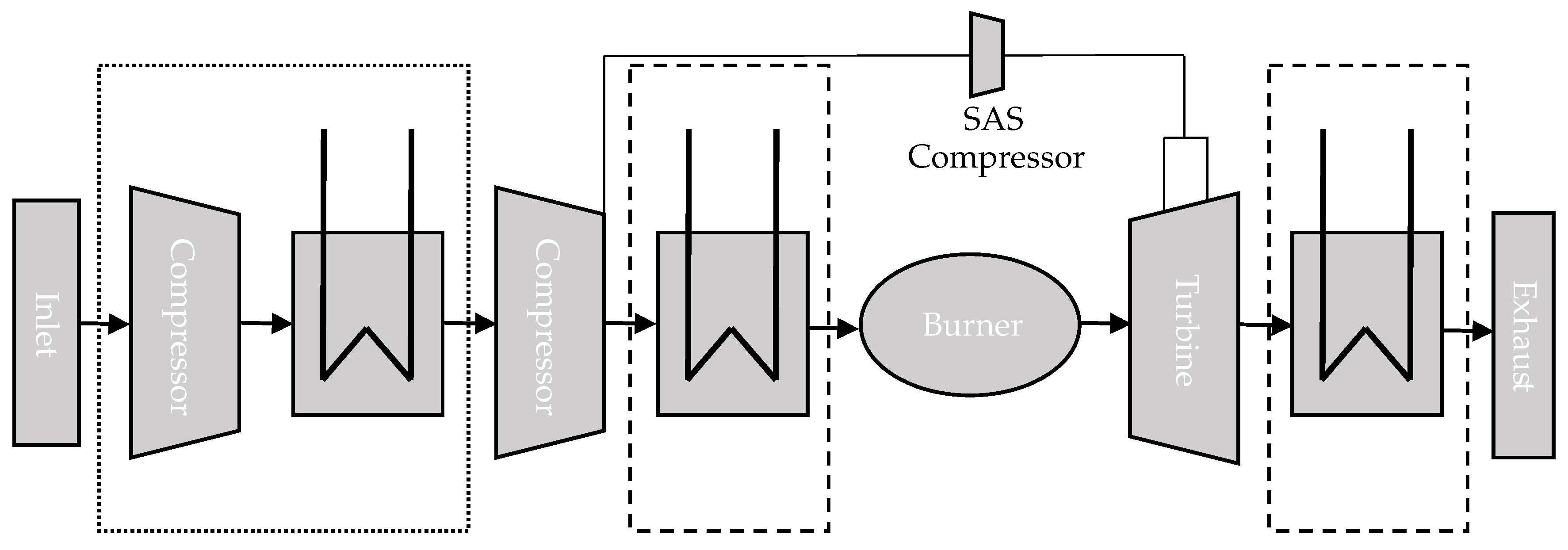
2.1.4. Intercooler and Recuperator

Combining an intercooler and a recuperator within a gas turbine results in an intercooled-recuperated gas turbine. The resulting setup is depicted in Figure 1 including the dotted and dashed lines. The assumed effectiveness and pressure losses were as defined for the cases above.

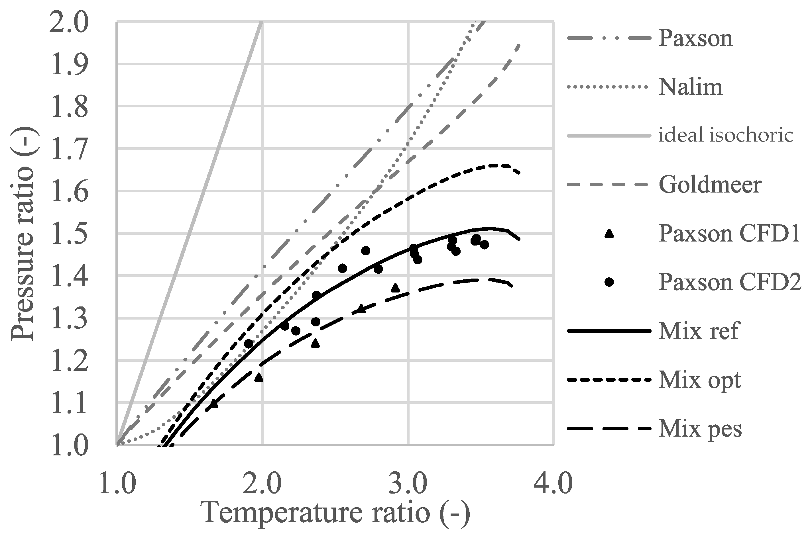
2.2. Combustor Model

The modeling of pressure gain combustion was crucial for this study. However, the single correct model for PGC did not exist. That is all the more especially true as many different approaches aim to increase pressure during combustion. For this steady-state zero-dimensional simulation (also the lumped volume approach), each component was represented by a transfer function or tabulated values in order to link inlet and outlet states. Functions for mass flow, total temperature, and total pressure were necessary. For PGC, the mass flow was simply the sum of inlet air flow and fuel flow. The outlet temperature was calculated as for conventional combustion from the energy balance. In GTlab-Performance, lookup tables created in the software Cantera were used to determine the outlet temperature for the equilibrium state. The difficulty, as indicated in the Introduction, was associated with the outlet pressure. This steady-state approach required a single value representative for the intermittent process. Therefore, only a few models were applicable, from which the following were implemented. For completeness, they are repeated here: the models provided by Paxson [28] and Goldmeer [18] calculate the pressure ratio (PR) from an enthalpy ratio (HR), which is given by the fuel flow. First, a non-dimensional heat is calculated giving the enthalpy ratio from an energy balance around the combustor (Equations (3) and (4)). The pressure ratio was then derived in Equation (5) using a tuning factor C, which was 0.12 according to Paxson and 0.105 according to Goldmeer.

$$q_0=\frac{LHV}{\left(1+AFR\right)\gamma R_g{T}_{in}}$$

(3)

$$HR=1+q_0\left(\gamma -1\right)\left(1-pf\right)$$

(4)

$$PR=H{R}^{\frac{C\gamma }{\gamma -1}}$$

(5)

The purge fraction $pf$ will not be used in this analysis and is set zero throughout this paper. However, this could represent a handle for off-design operation. A different model was defined by Nalim [15]. Outlet temperature $T_{out}$ and isochoric combustion temperature $T_B$ were calculated from the energy balance around the combustor (see Equation (6)). From this temperature, the isochoric pressure $p_B$ was found using an isochoric change of state (Equation (7)). The isochoric combustion was then followed by an isentropic expansion to the outlet condition. The outlet pressure $p_{out}$ was calculated using the outlet temperature $T_{out}$ and the isentropic relation in Equation (8).

$$Q=\dot{m}{c}_v\left(T_B-T_{in}\right)=\dot{m}{c}_p\left(T_{out}-T_{in}\right)$$

(6)

$$\frac{T_B}{T_{in}}=\frac{p_B}{p_{in}}$$

(7)

$$\frac{p_{out}}{p_B}={\frac{T_{out}}{T_B}}^{\frac{\gamma }{\gamma -1}}$$

(8)

Additionally, these authors inferred a PGC model that matched the CFD data provided by Paxson [9], which will be denoted as Mix. The results of CFD simulations by Paxson are also plotted in Figure 2 and were regarded as more accurate than the simple combustor models above. The complete setup of the experimentally-validated, one-dimensional, time-accurate, reactive, computational fluid-dynamics Euler solver was presented in [12]. Two different CFD datasets are available. The difference was associated with the fuel distribution within the combustion tube. For the data denoted Paxson CFD1, the tube was completely filled with the air fuel mixture, whereas an air buffer was present at the tube outlet in the dataset Paxson CFD2. The developed model from [19] was inferred from simplified pulse detonation combustion. A typical pulse detonation tube can be split into two combustion regimes. First, some sort of ignition source initiated a subsonic deflagration. The flame front encountered blockage bodies to eventually form a detonation, which consumed the remaining fuel towards to combustor tube outlet. The first part of the combustion can be modeled as isobaric combustion with some pressure losses, and the second can be modeled as isochoric combustion. Depending on the deflagration to detonation length (DDT), the whole process was more isobaric or isochoric. This idea was implemented in the combustor model. The developed PGC model calculated the combustor outlet temperature from the energy balance around the combustor using lookup tables. Secondly, a portion of the fuel denoted r was attributed to isobaric combustion $q_{cp}$. Again, lookup tables gave the temperature rise till $T_{cp}$ for this isobaric combustion (Equation (9)). This represents the temperature at the end of deflagration.

$$q_{cp}=FAR·r=c_p\left(T_{cp}-T_{in}\right)$$

(9)

The pressure loss $d{P}_{Loss}$ accounted for losses due to friction and heat addition as in Equation (10).

$$p_{cp}=p_{in}·d{P}_{Loss}$$

(10)

Finally, outlet pressure was calculated using Equation (11) and assuming an isochoric change of state.

$$p_{out}=\frac{T_{out}}{T_{cp}}·p_{cp}$$

(11)

The model behavior with 30% isobaric combustion ($r=0.3$) and a pressure loss of 20% ($d{P}_{Loss}=0.8$) agreed well with the data from Paxson at the same inlet temperature of 792 K and 24 atm, as depicted in Figure 2. However, the model deviated at higher temperature ratios (TR) from the data. Here, the stoichiometric combustion temperature limits at 2500 K were reached, leading to lower equilibrium temperatures. The performance in terms of pressure ratio against temperature ratio is depicted in Figure 2 for all introduced combustor models.

For gas turbine cycle analyses, the TR between 1.8 and 3 was relevant [19]; therefore, the shortcomings of the Mix model towards high TR were negligible. In order to assess the sensitivity of the gas turbine design with respect to different PGC implementations, an optimistic and pessimistic version of the developed model with respect to combustor performance will be created. For the optimistic model (Mix opt), $r=0.24$ was selected, and for the pessimistic (Mix pes) $r=0.36$. This means that there was 20% more isochoric combustion for the optimistic case, and in the pessimistic case, there was 20% more isobaric combustion. The effect on PR is also depicted in Figure 2. The ideal isochoric model used the mix model with $r=0.0$. The complete fuel was burnt under isochoric conditions. The isobaric combustion was modeled with a pressure loss of 5% and a combustion efficiency of 99%. For PGC, a combustion efficiency of 100% was assumed.

2.3. Optimization Setup

The optimizations were run on the in-house software IPSM (Interface for performance and SAS modeling [31]) and identified the optimum gas turbine designs for predefined constraints. For this study, the first constraint was shaft power, which was held constant at $6.63$ MW. The second constraint was the turbine blade temperature calculated by Equation (1). For this study, three different temperatures were investigated: a very conservative blade temperature of 1000 K, a reasonable 1100 K, and a high 1200 K. The temperature range was identified based on data provided by [32]. Additionally, the secondary air mass flow was limited to a maximum of 35% of the engine inlet mass flow. The three constraints are listed in

Table 3. Constraints for optimizations.

Output power	=	6.63 MW
Turbine blade temperature	≤	1000 K, 1100 K, 1200 K
Cooling mass flow/engine mass flow	≤	35%

.

Depending on the gas turbine cycle, the optimization had two or three variables. For the simple and recuperated cycle, engine mass flow and compressor pressure ratio were the degrees of freedom. For the intercooled and intercooled-recuperated engine, the second compressor pressure ratio was an additional variable. The parameter spaces were {2, 50} kg/s for engine mass flow and {2, 50} for the compressor pressure ratio. Here, the overall compressor pressure ratio was limited to 50 for intercooled setups. Engine mass flow as a variable was selected because it represented the engine size. Furthermore, engine mass flow directly provided the specific work, because the power output was held constant. Compressor pressure ratios were selected as the main thermodynamic parameter of influence. Since blade metal temperature and power output were selected as constraints, this setup calculated TET, which delivered the required power output and did not exceed the blade temperature margin. The objective function of the optimization was thermal efficiency, defined as follows:

$${\eta }_{th}=\frac{P{W}_{output}}{{\dot{m}}_{fuel}·LHV}$$

(12)

The workflow applied for the optimizations is sketched in Figure 3. It included the optimization loop providing the degrees of freedom to the gas turbine performance model in order to maximize the thermal efficiency ${\eta }_{th}$ and an embedded iterative process. The latter ensured the coolant flow matched the defined metal temperature. The required cooling flow was calculated using Equation (1). The input parameters were directly taken from the performance simulation results. The calculated mass flow was used as a new input to the performance model. This loop was iterated till convergence was reached. The optimization combined two different types of algorithms sequentially. First, an in-house-developed evolutionary algorithm was applied to the optimization problem in order to browse the parameter space for promising regions. Subsequently, a gradient-based algorithm continued the optimization on a set of the best solutions found by the evolutionary algorithm.

3. Results and Discussion

Optimizations were conducted of the simple gas turbine (GT), intercooled GT, recuperated GT, and intercooled-recuperated GT for blade temperature constraints of 1000 K, 1100 K, and 1200 K, as well as for the following combustor models: isobaric, ideal isochoric, Mix ref, Paxson, and Nalim. The model of Goldmeer was not considered further since it is similar to Paxson’s model. The Mix opt and Mix pes models were only considered for the simple cycle. The Results Section is divided into five parts. First, the overall results including the thermal efficiency and specific work of the different setups are compared. Here, the effects of different blade temperatures are analyzed. Secondly, each gas turbine setup is analyzed and gas turbine specifications for optimum design are presented. This is done for the simple cycle gas turbine in Section 3.2, which serves as a reference for comparison with advanced cycles. Section 3.3 discusses the intercooled cycle. In Section 3.4, the results of the recuperated cycle are presented, and lastly, Section 3.5 deals with the combined intercooled-recuperated cycle. The analysis of the advanced cycles was limited to a blade temperature constraint of 1100 K. For this boundary condition, cycle design parameters such as OPR (overall pressure ratio including combustion) and TET, but also the SAS mass flow and SAS compressor power were included. Furthermore, insights into the optimum pressure ratio split between LPC and HPC are presented where applicable. Additionally, heat exchanger inlet temperatures are given for the advanced cycles.

3.1. Thermal Efficiency and Specific Work

Absolute thermal efficiency after the optimizations are depicted for the different cycles and combustor models for a blade temperature constraint of 1100 K in Figure 4. For all cycles, isobaric combustion resulted in the lowest efficiencies (right-hand side). Instead, the highest efficiencies were found for ideal isochoric combustion (left-hand side). While Paxson’s model gave the highest efficiencies within the realistic PGC representations (Paxson, Nalim, and Mix ref) followed by Nalim’s model and the Mix ref model, they only differed by 1.5 PP. If different cycle setups were compared, the simple cycle resulted in the lowest efficiencies. The intercooled and recuperated cycle were almost level, and the intercooled-recuperated cycle (Int-rec) achieved the highest efficiencies. The ideal isochoric combustion in an intercooled-recuperated cycle could increase the efficiency by almost 20 PP compared to a simple cycle with constant pressure combustion. Realistic representations of PGC still achieved an efficiency gain in the intercooled-recuperated cycle of 15.6 PP.

Figure 5 presents possible synergies of PGC in advanced thermodynamic cycles at different blade temperature constraints. Here, thermal efficiency gains are depicted for the different types of combustion and cycles. First, the blade temperature constraint of 1100 K was analyzed. The efficiency gain was defined as the difference between simple cycle thermal efficiency and thermal efficiency of the advanced cycle using the same type of combustion. Figure 4 illustrates the efficiency for various models and cycles at $T_{mat}$ of 1100: intercooling, for example, increased the efficiency for isobaric combustion from 37.36% to 40.89%. This efficiency gain of 3.52 PP is depicted in Figure 5. The efficiency gain for PGC modeled by Nalim in an intercooled cycle was slightly higher (from 44.04–47.41%). Therefore, applying PGC in an intercooled cycle can lead to higher efficiency gains, and it can create synergies. This is marked exemplary by the green arrow in the zoom up. No synergies were created with the model of Paxson (red arrow). In general, the intercooled cycle was favorable for PGC since it had a lower combustor entry temperature, which allowed for more heat input in the combustor, resulting in higher pressure ratios. However, taking ideal isochoric combustion, the efficiency gain was smaller. Above a relative proportion of the combustor pressure ratio to overall pressure ratio, the efficiency gains due to intercooling were reduced. A possible explanation was that ideal isochoric combustion favored low TET and OPR, but had a high pressure increase over the combustor (compare with the detailed results in Section 3.3). Hence, the compressor pressure ratios and powers were low, reducing the potential of intercooling.

Looking at the recuperated cases in Figure 5 (middle), isobaric combustion yielded the highest efficiency gain. Applying PGC did not create synergies, but subtracted some of the efficiency gain present at isobaric combustion. Applying PGC reduced both turbine exit temperature and compressor exit temperature. However, the former was more affected. As a result, the driving temperature difference for recuperation was reduced for PGC (compare with the detailed results in Section 3.4).

The intercooled-recuperated engine setup improved gas turbine thermal efficiency for isobaric combustion (11 PP) the most. Using realistic PGC representations, the efficiency rose by ≈9.8 PP. For ideal isochoric combustion, the improvement was only about 6.6 PP. Hence, applying combined recuperation and intercooling was more beneficial for isobaric combustion than for PGC. For a blade temperature constraint of 1100 K, it can be concluded that intercooling seemed favorable for PGC because thermal efficiency gains could be increased. Recuperation and combined intercooling and recuperation reduced the efficiency gains for PGC compared to conventional isobaric combustion. Still, the advanced cycles achieved higher absolute efficiencies for all types of combustion compared to the simple gas turbine cycle.

For a temperature constraint of 1200 K, the discussed effects were even stronger (see the same figure). All realistic PGC models increased the efficiency gain for an intercooled GT (+4 PP compared to only +2.7 PP for isobaric combustion) and lowered the gain for recuperated and intercooled-recuperated engines. Especially, the latter was negatively affected. At 1200 K, the efficiency gain was 1 PP less for PGC in an intercooled-recuperated engine than for 1100 K. It can be concluded that higher acceptable blade temperatures improved the potentials for PGC in an intercooled engine, but reduced them in an intercooled-recuperated engine. Efficiency gains of the recuperated cycle did not seem sensitive to different blade temperature constraints.

Results of the optimizations at a blade temperature constraint of 1000 K in Figure 5 show that PGC reduced the efficiency gains in the combined intercooled-recuperated cycle. On average, the reduction was similar to 1200 K. For the intercooled cycle, efficiency gains were still present for Nalim’s model and the Mix ref model, but smaller.

Figure 6 depicts the specific work of the gas turbine for the different cycles and combustion types. PGC could increase specific work by almost 50% in advanced cycles. Particularly, intercooling and combined intercooling and recuperation achieved high improvements, as already announced in the Introduction. Large specific work gains were found compared to the simple and recuperated cycle. However, comparing the specific work for different combustion models was difficult, as no trend was visible. Apparently, the behavior of the different combustor models led to completely different operating points in terms of the combustor temperature ratio and pressure ratio for optimum cycle efficiency.

3.2. Simple Cycle Gas Turbine

Detailed results of the simple cycle optimizations at a turbine blade temperature of 1100 K can be found in [19]. Therefore, emphasis will be put on the effect that different blade temperature constraints have on the optimized gas turbine specifications and thermal efficiency for the simple cycle GT. Figure 7 presents the relative key performance parameters for each combustor model after the optimization. The reference values for each combustor model are summarized in

Table 4. Reference values at $T_{mat}=1100$ K for Figure 7.

	Isobaric	Isochoric	Mix Opt	Mix Ref	Mix Pes	Paxson	Nalim
Thermal efficiency (%)	37.36	50.51	42.71	41.92	41.17	44.04	42.30
Specific work (MJ/kg)	0.3084	0.3097	0.3107	0.3033	0.2978	0.2606	0.3570
Pressure ratio (−)	24.79	12.18	17.23	18.34	18.89	17.63	16.81
TET (K)	1608.8	1169.87	1390.26	1401.94	1407.19	1232.89	1540.9

. First, consider a blade temperature of 1000 K in Figure 7 (bottom). Relative changes compared to the optimization for a blade temperature of 1100 K are shown. The 9% reduction in blade temperature led to lower thermal efficiencies. This reduction had a stronger effect on a cycle with isobaric combustion (−8.6%) than on a cycle with isochoric combustion (−5%). PGC could enable lower blade temperatures with increased creep life at an acceptable efficiency penalty. Furthermore, the specific work of the cycle was also reduced for a lower blade temperature. Here, the PGC cases were more affected than the isobaric case. The compressor pressure ratios were most affected according to Figure 7 and were reduced by up to 25%. However, this sensitivity for optimum thermal efficiency was already present for isobaric combustion and was not altered by realistic PGC. Furthermore, the TET did not decrease proportional to the decrease in blade temperature. Instead, TET was reduced by only ≈3% for the isobaric and realistic PGC cases. Here, the reduced temperature constraint was met by a small reduction of the TET and an increase of the blade cooling. In the isochoric case, TET was reduced by almost 10%, which was more than the reduction of the blade temperature limitation. This larger reduction decreased the cooling mass flow requirements, which eventually resulted in a higher cycle efficiency. Apparently, the power requirement for the compression of cooling air had a huge penalty on thermal efficiency for the ideal isochoric case. This was because ideal isochoric combustion gave pressure ratios across the combustor, which were much higher compared to the other combustor models (compare Figure 2).

In contrast to a reduction in blade temperature as discussed above, Figure 7 (top) depicts the results at a higher blade temperature limitation of 1200 K. The design space was enlarged, resulting in higher thermal efficiencies. The isochoric cycle was not very sensitive to this constraint, as already shown. Indeed, it only resulted in a thermal efficiency gain of 4.4%. The efficiency of the isobaric cycle, in turn, improved by more than 7%. Consequently, technology improvements leading to higher acceptable blade temperatures or improved cooling technologies will not raise cycle efficiency as much for PGC as for conventional combustion.

Comparing the behavior of the PGC models in Figure 7, ideal isochoric and all Mix models behaved consistently for different temperature constraints. For the PGC models by Nalim and Paxson, that was not the case. Lower and higher temperature constraints led to completely different cycles. For a blade temperature of 1200 K, the compressor pressure ratio was only increased by 10%, whereas for a blade temperature of 1000 K, the pressure ratio was reduced by almost 30%. That was because for optimum cycle efficiency, the combustor operating points differed significantly. The corresponding temperature-entropy diagrams with Nalim’s and the Mix ref combustor models for all three blade temperature constraints are depicted in Figure 8. Nalim’s model favored high combustor temperature ratios because the pressure ratio rose exponentially (see Figure 2), whereas the Mix ref model showed an asymptotic behavior with a rising combustor temperature ratio. The blade temperature constraint of 1200 K drove Nalim’s model to very high temperature ratios. A high cooling flow was necessary, which was indicated by the loss in temperature before the flow was expanded in the turbine. That was not the case for the Mix ref model. A consistent shift to higher compressor pressure ratios and TET with higher blade temperatures is visible in Figure 8. The explanation given for Nalim’s model applies also to Paxson’s model.

From Figure 7, the difference in thermal efficiency of the Mix models is hardly perceptible. Figure 9 elaborates on that. The relative change in efficiency compared to the Mix ref model is depicted for the Mix pes model (higher fraction of isobaric combustion and longer DDT length) and the Mix opt model (higher fraction of isochoric combustion and shorter DDT length) at different blade temperature constraints. At lower temperatures, the relative difference in thermal efficiency was larger. Hence, DDT length was more important at lower rather than higher temperature constraints.

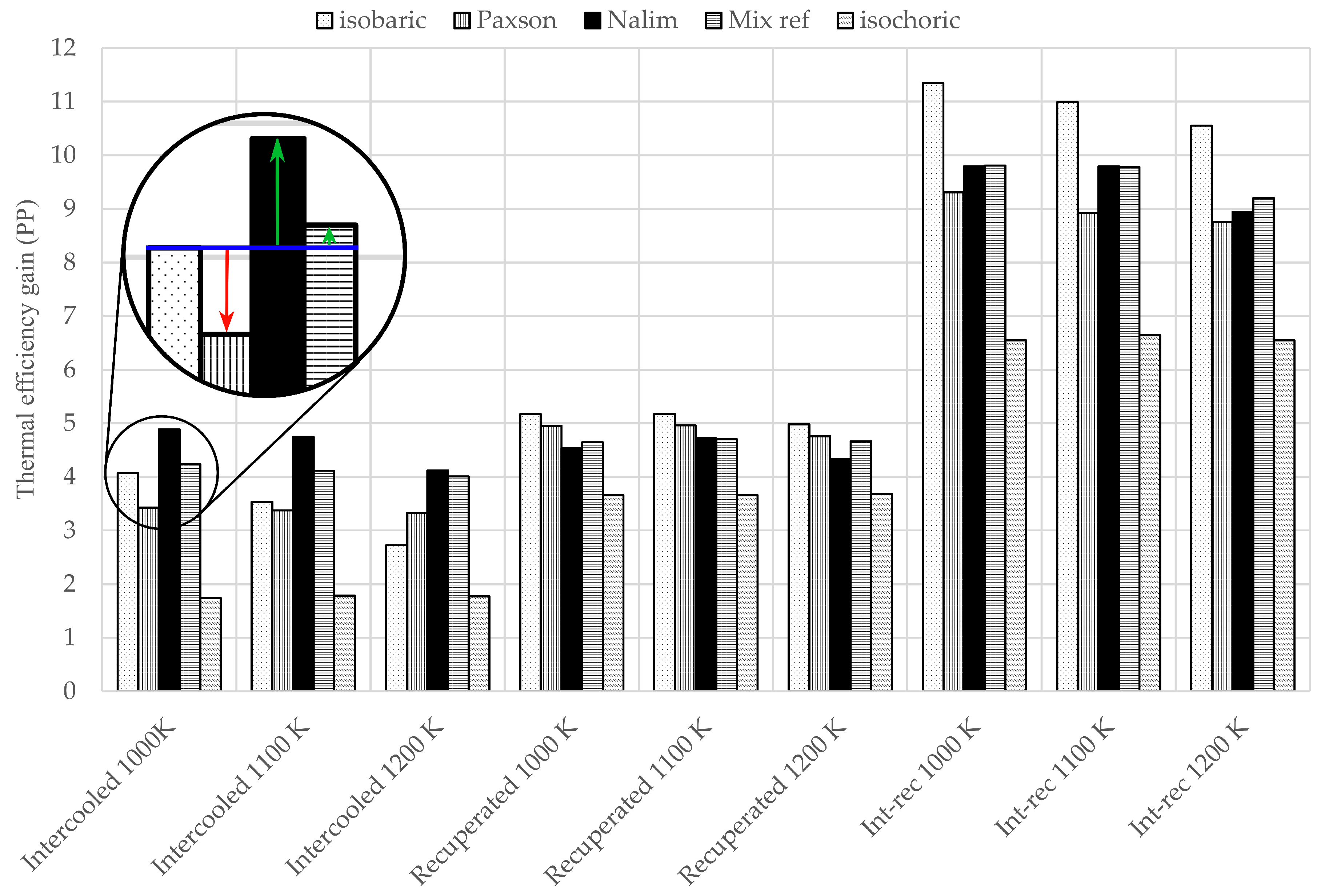
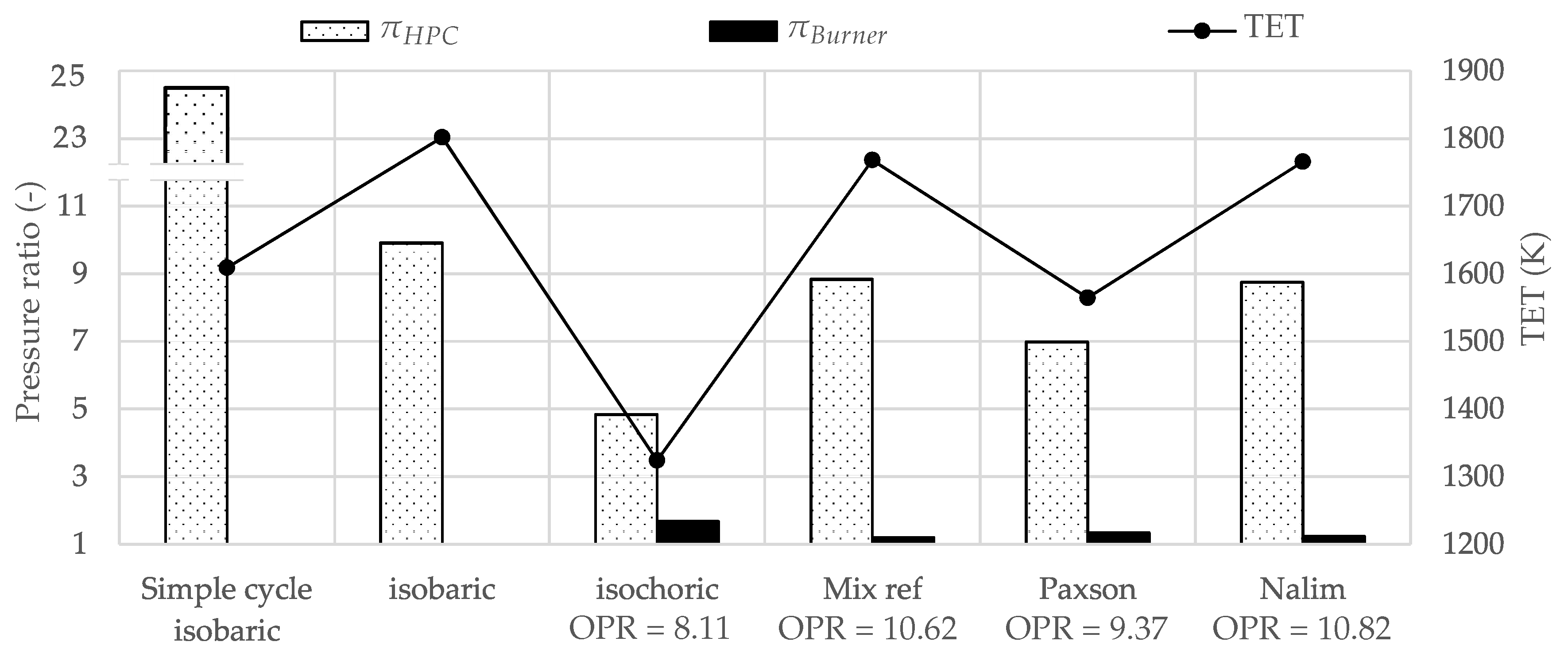
3.3. Intercooled Gas Turbine

The effect of intercooling on the thermodynamic cycle at a blade temperature constraint of 1100 K is presented in Figure 10 for pressure ratios on the primary axis. Compared to the simple cycle with isobaric combustion (${\pi }_{HPC}=24.78$), intercooled cycles had overall pressure ratios (OPR) at least twice as high. The intercooled cycle with isobaric combustion shifted most of the compression to the HPC for optimum efficiency. The pressure ratios for the compressors were substantially reduced for the isochoric case. In the combustor, additional compression took place to reach the same OPR as with isobaric combustion. The realistic PGC models required OPR in excess of 57. Both LPC and HPC pressure ratio were increased. Comparing these models, LPC and combustor pressure ratios rose from the Mix ref to Paxson’s to Nalim’s models. The opposite happened with the HPC pressure ratios for optimum efficiency. Hence, the thermodynamic cycles were again very sensitive to the selected combustor model. In Figure 10, TET is also plotted for the different combustor models. Intercooling allowed for a reduction in TET for isobaric combustion. This was not the case with realistic PGC. The TET for realistic PGC models was similar to a TET in a simple cycle with isobaric combustion.

Intercooling reduced the SAS mass flow for isobaric combustion from 24% of the engine mass flow to 11%. However, applying PGC required between 21% and 25% cooling air again. Compared to the simple cycle with isobaric combustion plotted on the left-hand side in Figure 11, intercooling combined with realistic PGC maintained the required SAS mass flows. The power requirement of the SAS compressor to overcome the pressure gain in the combustor was in the order of 5%. That was a result that was already found in [19] for the simple cycle with PGC. The intercooler inlet temperature of the hot side was also plotted in Figure 11. The LPC pressure ratios were higher for realistic PGC, leading to higher inlet temperatures into the intercooler. Hence, more specific heat was removed in the given setup with constant intercooler outlet temperature. This explains the efficiency gain of Nalim’s model compared to isochoric combustion in Figure 5.

3.4. Recuperated Gas Turbine

Figure 12 depicts the pressure ratios for the recuperated cycle. Recuperator performance was driven by the temperature difference of the cold and the hot side. More heat was transferred if cold side temperatures were low. That is why the compressor pressure ratios for the recuperated cases were small compared to the other cycles. Additionally, recuperation increased the combustor inlet temperature, which combined with the blade temperature constraint restricted the temperature ratio in the combustor. Hence, also the pressure ratios in the combustor were rather small, resulting in OPR below 11. One could expect low TET from this, since TET and OPR were coupled, but recuperation required not only low cold side temperatures, but also high hot side temperatures. In order to provide high turbine outlet temperatures, TET were similar to the simple cycle TET with isobaric combustion and the intercooled cycle TET with PGC. Only the ideal isochoric case provided a huge reduction in TET.

Figure 13 presents SAS and heat exchanger specifications. Adding recuperation to an engine with isobaric combustion only reduced SAS mass flow by 2 PP. However, applying recuperation with PGC reduced the SAS mass flows. Here, cycles using the model of Paxson required a SAS mass flow of only 15%, and with the ideal isochoric combustion, a mass flow of 7.5% sufficed. In addition, the recuperated setup lead to a substantial reduction in the SAS compressor power. The power requirement for the SAS compressor was below 2.5% of the output power. That was half of the power required for the intercooled cycle. The reduced pressure gain in the combustor for recuperated cycles was responsible for this. Figure 13 depicts also the inlet temperatures to the recuperator heat exchangers. The temperature differences were in the same order for all cycles for optimum efficiency even though the TET varied between realistic PGC representation by more than 200 K. Thus, the transferred specific heat through the recuperator was almost equal for all models.

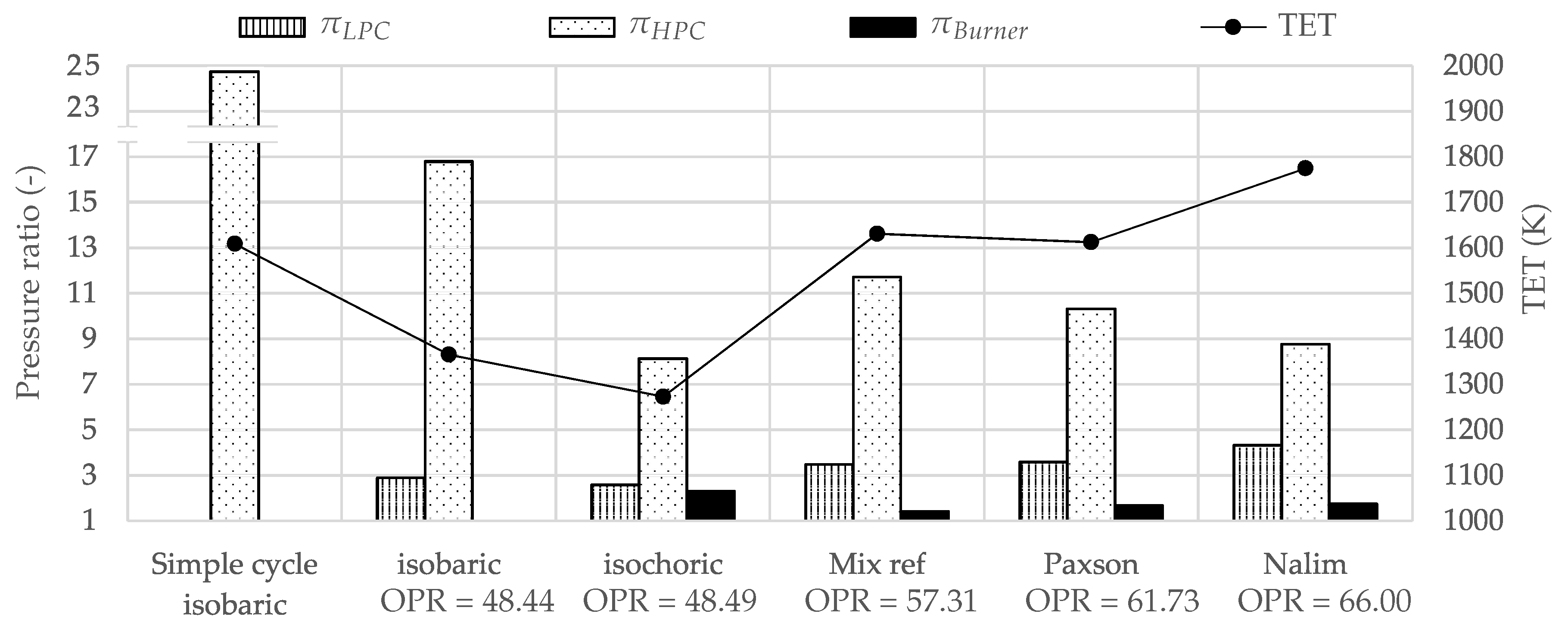
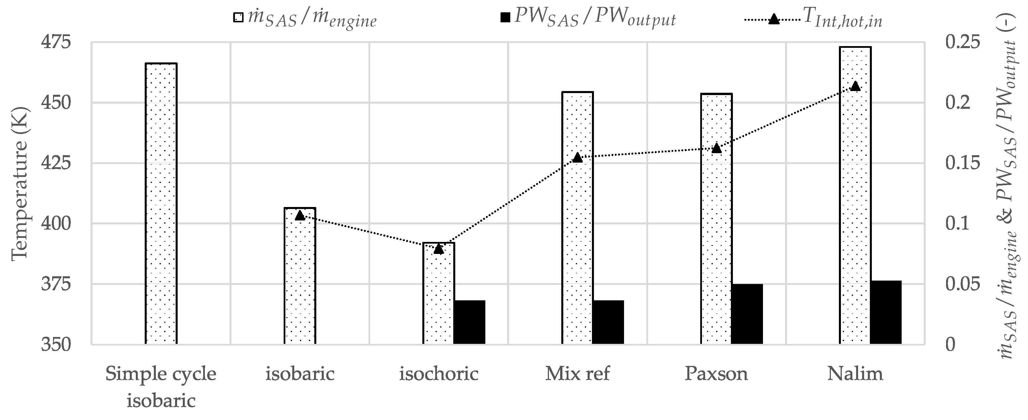
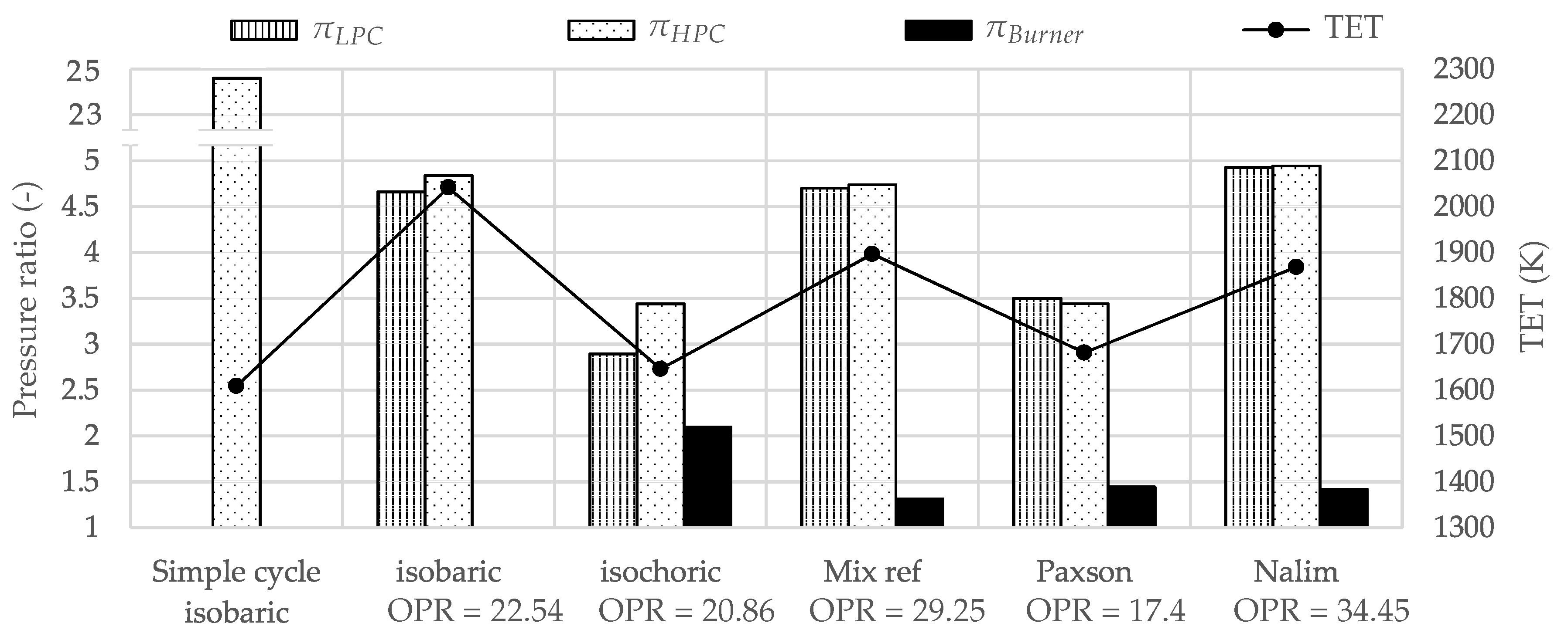
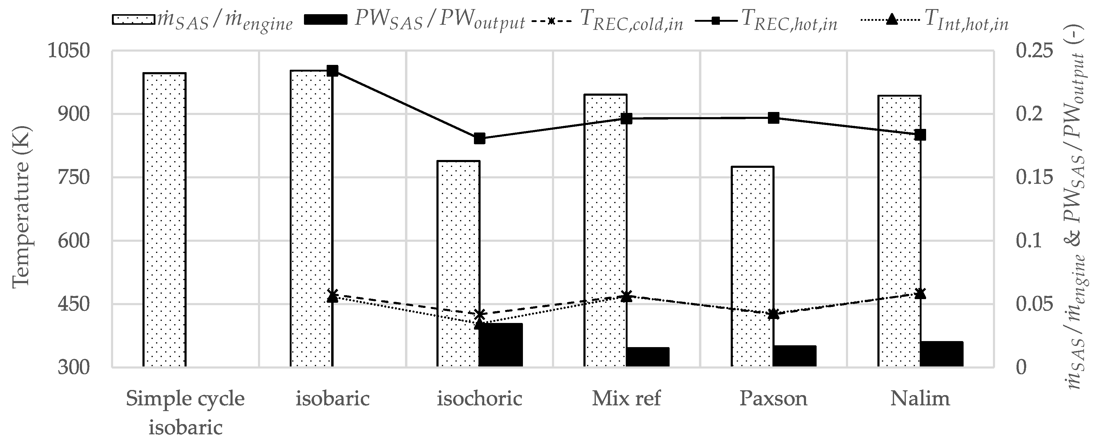
3.5. Intercooled-Recuperated Gas Turbine

For the intercooled-recuperated cycles, pressure ratios and TET are plotted in Figure 14 for a blade temperature constraint of 1100 K. Overall pressure ratios were between those of the intercooled cycles and the recuperated cycles. The HPC and LPC pressure ratios for optimum thermal efficiency highly depended on the selected combustor model. Paxson’s model favored a low pressure ratio, whereas the Mix ref model and Nalim’s model favored high pressure ratios. This was due to the different underlying mathematical formulations of the combustor models. In contrast to intercooling, LPC and HPC pressure ratios were very close. The pressure ratios of the combustor as a result of the available temperature ratios were smaller with combined intercooling and recuperation compared to pure intercooling because of recuperation. However, they were also higher compared to pure recuperation because of intercooling. Compared to the simple cycle with isobaric combustion, pressure ratios of the compressors were in the same range for all combustors models, but the ideal isochoric model and Paxson’s model.

The intercooled-recuperated cycles had the highest TET. They were even above the simple cycle TET with isobaric combustion. Blade temperature margins were still met, since cooling air temperatures were low due to intercooling. The coupling of TET with OPR is again visible in the data of Figure 14.

Figure 15 depicts SAS specifications and intercooler and recuperator inlet temperatures. The SAS mass flow increased slightly when isobaric combustion was coupled with combined intercooling and recuperation. However, using PGC, reduced the SAS mass flow below 21%. Again, the ideal isochoric representation and the model of Paxson required SAS mass flows of 16% of the engine mass flow. In addition, the SAS power requirement was again reduced compared to the intercooled cycle, and only ≈2.5% of the output power was required. The reduced pressure ratio of the combustion and low cooling air temperatures enabled this trend for intercooled-recuperated cycles. Figure 15 also presents inlet temperatures of the heat exchangers. The driving temperature differences between the recuperator hot and cold side were similar for all computed combustor models and in the same range compared to purely recuperated cycles. The intercooled inlet temperatures were almost identical to the recuperator cold side inlet temperatures because LPC and HPC pressure ratios were almost equal. However, compared to pure intercooling, they were sightly increased by ≈30 K. More specific heat was removed from the cycle.

In summary, the cycle designs for optimum thermal efficiency were very different. The underlying combustor model and selected advanced cycle had a huge impact on engine mass flow (equivalent to specific work in Figure 6), pressure ratios, TET, and SAS specifications. Only specific heat of the heat exchangers was rather insensitive to the combustor model. Still, the general guidelines for optimum cycle design were identified and the potentials in thermal efficiency quantified.

4. Conclusions

This paper presented comprehensive optimization studies for pressure gain combustion in advanced thermodynamic cycles with intercooling and recuperation. The objective of these studies was to quantify the possible potentials of such a combination, as well as to identify promising gas turbine designs for optimum thermal efficiency. To shed light on this, different pressure gain combustion models for an application in steady–state gas turbine performance simulations were identified and implemented in gas turbine models for conventional, intercooled, recuperated, and intercooled-recuperated engines. These were optimized regarding thermal efficiency for a constant power output at three different first stage turbine blade temperatures. The following conclusions can be drawn:

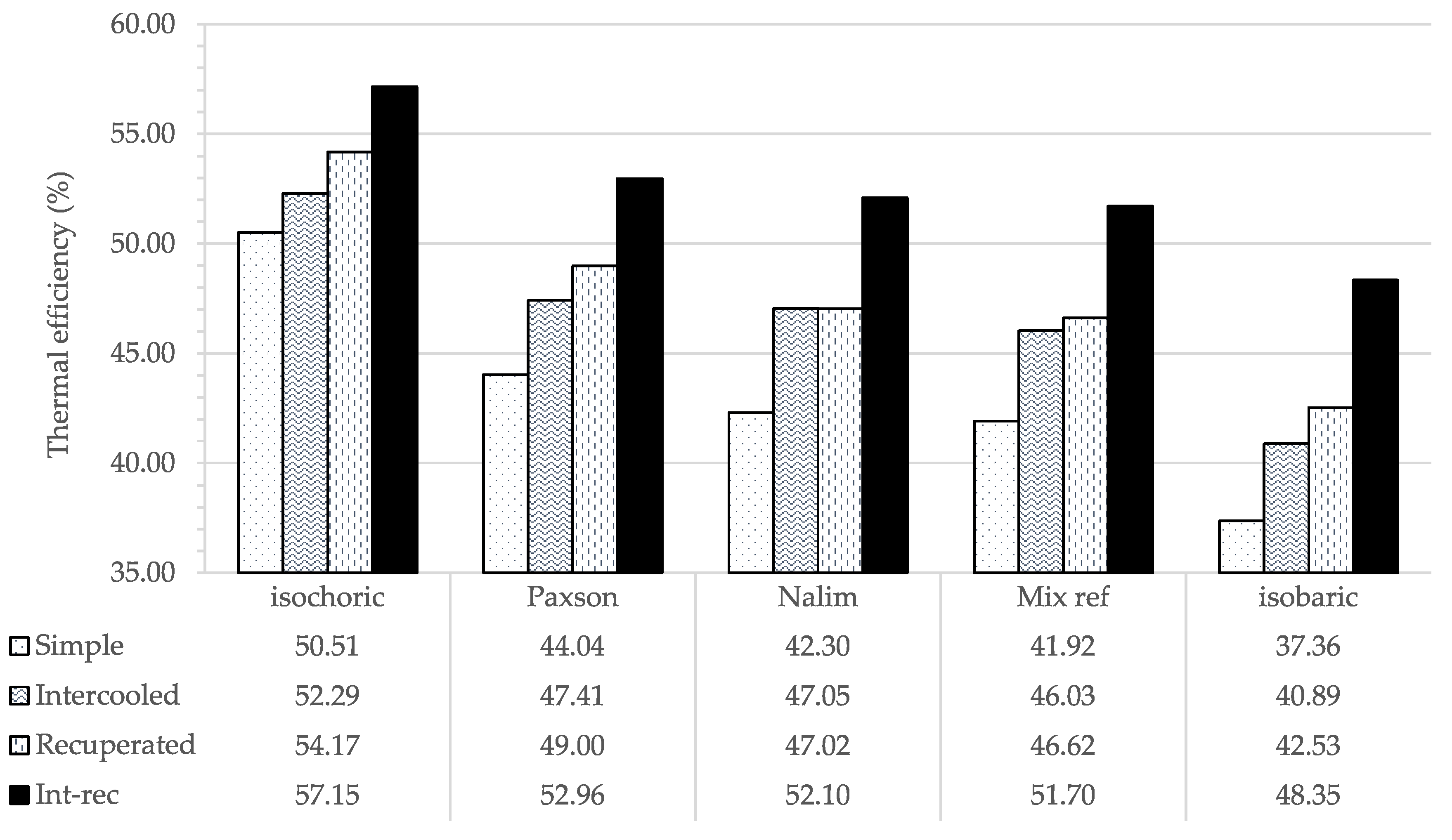
• Advanced thermodynamic cycles improved thermal efficiency for all combustion types. An intercooled-recuperated engine using Paxson’s PGC model achieved a thermal efficiency increase of 15 PP compared to a simple gas turbine with isobaric combustion. Pure intercooling with Paxson’s combustor model increased the efficiency by 10 PP. However, the efficiency gain through recuperation and combined intercooling and recuperation with PGC was lower than for the same cycle with isobaric combustion. Only in the intercooled cycle did PGC achieve higher efficiency gains compared to isobaric combustion. Intercooling was therefore favorable for PGC and may create synergies. This behavior was amplified when higher turbine blade temperatures were acceptable.
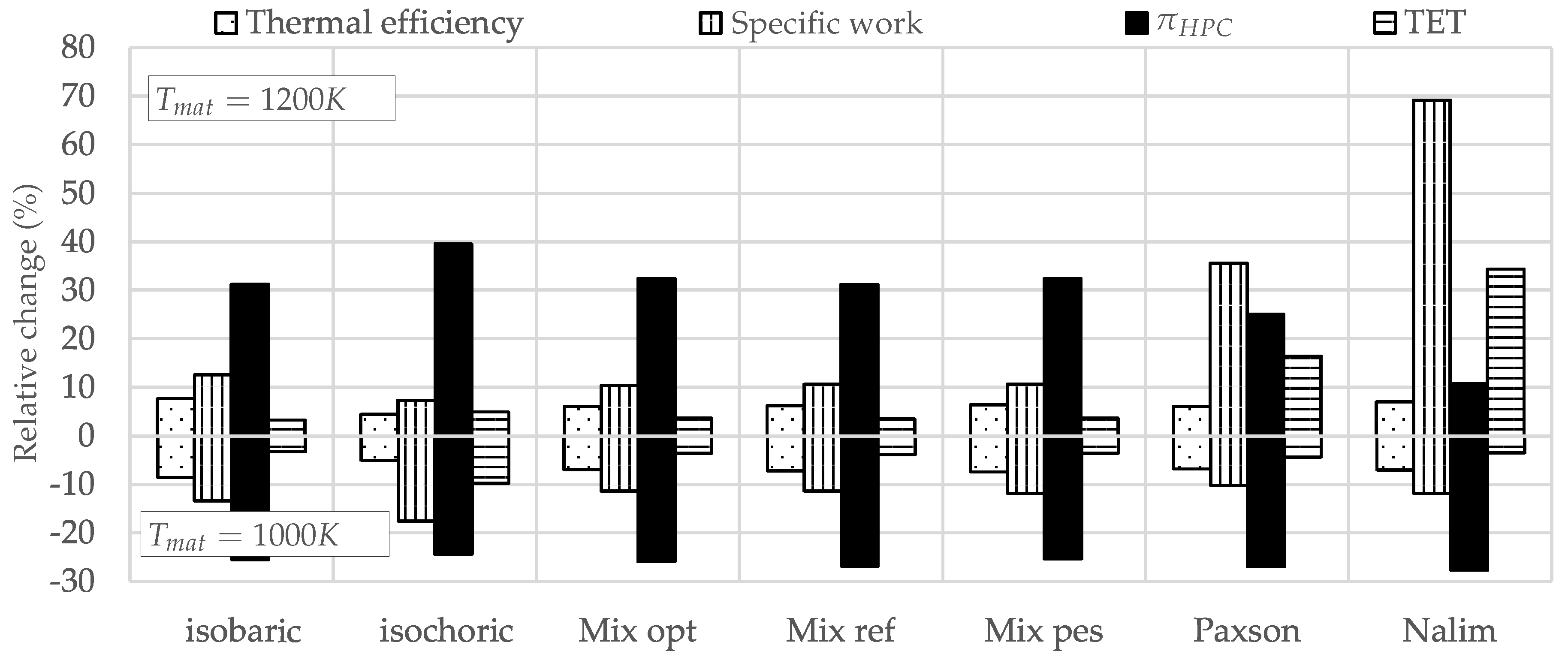
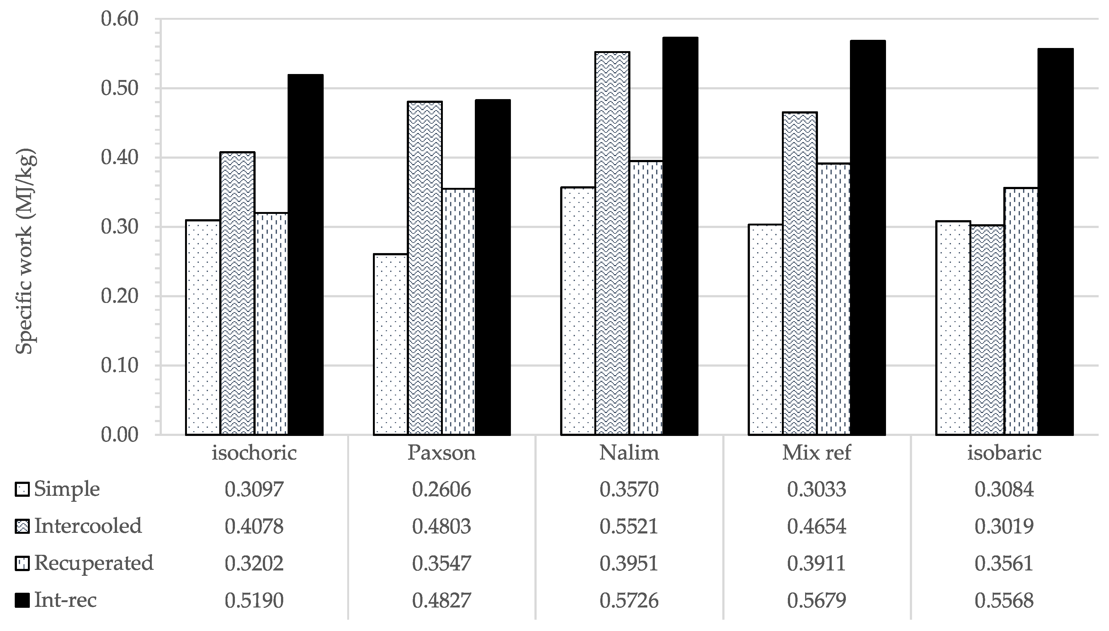
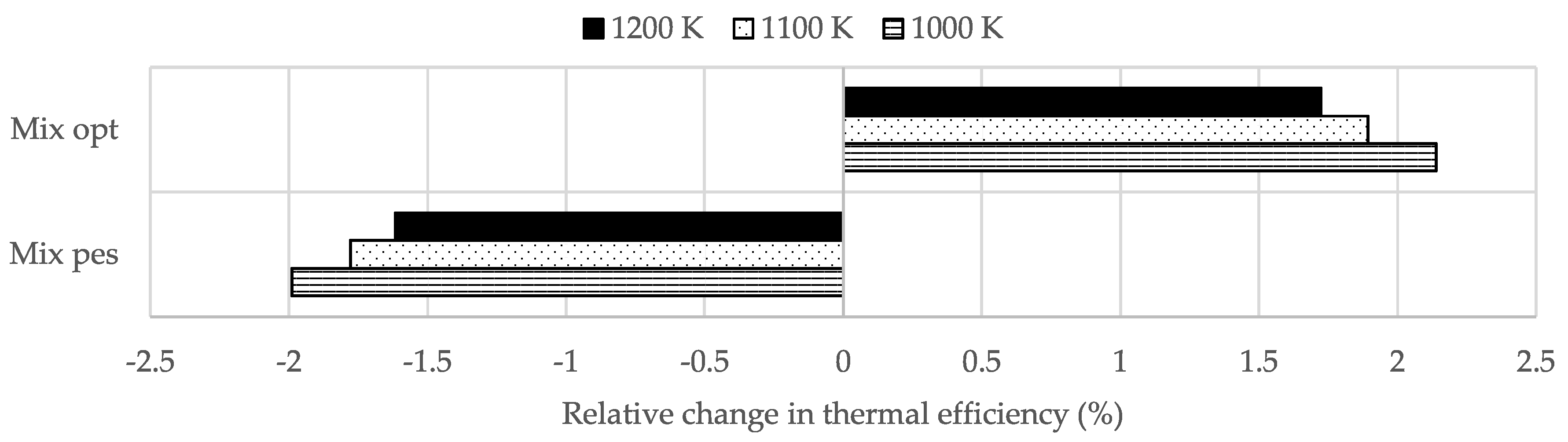
• In comparison to PGC, isobaric combustion attained higher thermal efficiency gains in a simple cycle when the allowable blade temperature constraint was increased. In contrast, reducing the blade temperature constraint resulted in a lower efficiency penalty for PGC than for isobaric combustion. This could affect the compromise between cycle efficiency, which favors high turbine entry temperatures, and blade creep life, which favors low temperatures. In addition, a lower blade temperature constraint reduced the specific work more significantly for PGC than it did for isobaric combustion. Comparison of the Mix models led to the conclusion that the effect of DDT length on thermal efficiency was stronger at lower blade temperature constraints.
• The optimum thermodynamic design of an advanced gas turbine with pressure gain combustion can be summarized as follows: The optimization of the intercooled-recuperated cycles yielded OPR between 17 and 35. The LPC and HPC pressure ratios were equal for optimum thermal efficiency. The optimized intercooled cycles had OPR in excess of 48, which was almost twice as high as the intercooled-recuperated cycles. Furthermore, most of the compression took place in the HPC. The recuperated cycles had the lowest OPR with values below 11. The driving temperature difference of the recuperator was almost identical for all combustor models and did not differ from the intercooled-recuperated cycles. The TET for optimum thermal efficiency did scatter, and no general design guideline can be given for advanced cycles.
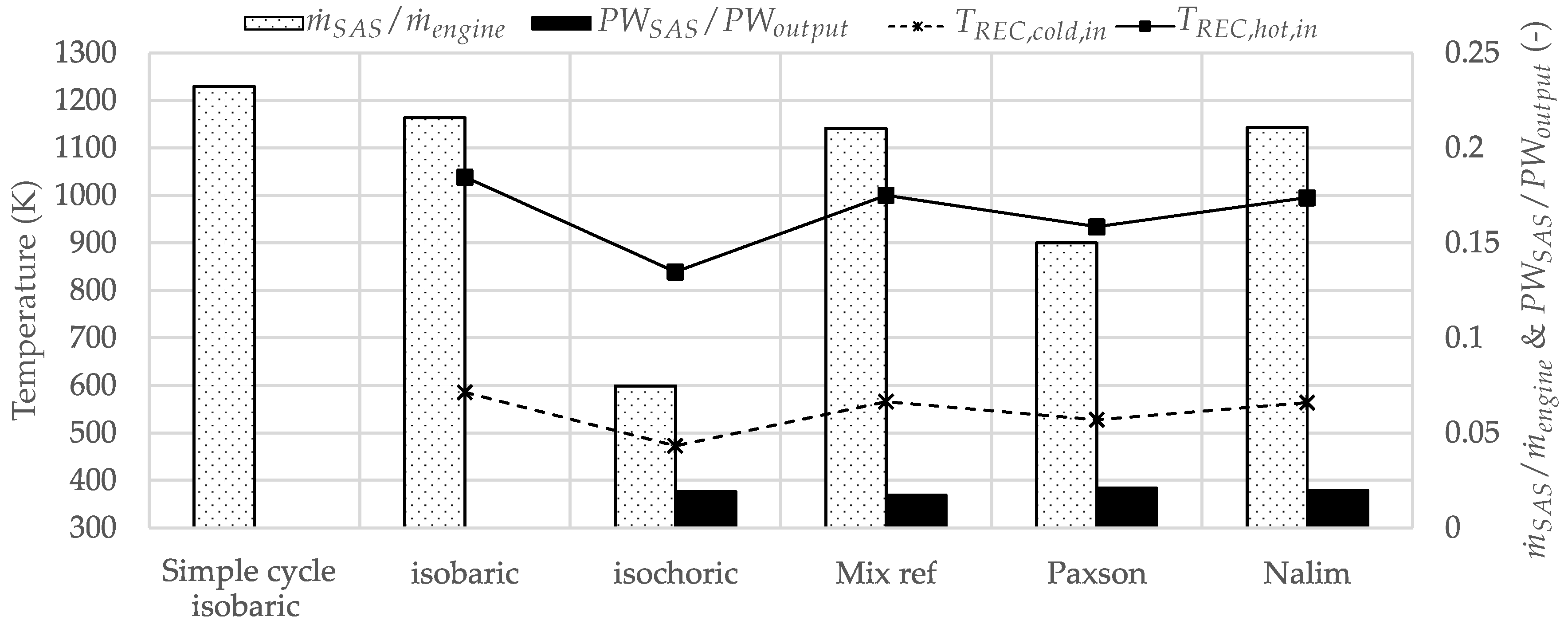
• The required SAS mass flow depended on the advanced cycle and on the underlying combustor model. In general, compared to a cooling mass flow requirement of 20% computed for the simple cycle with isobaric combustion, intercooling maintained this value, and recuperation and combined intercooling and recuperation lowered the value by at least 2 PP and 1.5 PP, respectively. Furthermore, the SAS compressor power requirement could be reduced with recuperation by roughly $50\%$ which is 2.5% of the output power.
• The different combustor model performances resulted in very different optimum cycle designs. This stresses the importance of reliable steady-state combustor models, which require more research.

References

1. Grönstedt, T.; Irannezhad, M.; Lei, X.; Thulin, O.; Lundbladh, A. First and second law analysis of future aircraft engines. J. Eng. Gas Turbines Power 2014, 136, 031202. [Google Scholar] [CrossRef]
2. Heiser, W.H.; Pratt, D.T. Thermodynamic Cycle Analysis of Pulse Detonation Engines. J. Propuls. Power 2002, 18, 68–76. [Google Scholar] [CrossRef]
3. Perkins, H.D.; Paxson, D.E. Summary of Pressure Gain Combustion Research at NASA; NASA TM-2018-219874; NASA: Washington, DC, USA, 2018. [Google Scholar]
4. Walsh, P.P.; Fletcher, P. Gas Turbine Performance; John Wiley & Sons: Hoboken, NJ, USA, 2004. [Google Scholar]
5. Carniere, H.; Willocx, A.; Dick, E.; Paepe, M.D. Raising cycle efficiency by inter cooling in air cooled gas turbine. Appl. Therm. Eng. 2006, 26, 1780–1787. [Google Scholar] [CrossRef]
6. Boggia, S.; Rüd, K. Intercooled recuperated gas turbine engine concept. In Proceedings of the 41st AIAA/ASME/SAE/ASEE Joint Propulsion Conference & Exhibit, Tucson, AZ, USA, 10–13 July 2005; p. 4192. [Google Scholar]
7. Paxson, D.E.; Kaemming, T. Influence of unsteadiness on the analysis of pressure gain combustion devices. J. Propuls. Power 2014, 30, 377–383. [Google Scholar] [CrossRef]
8. Vutthivithayarak, R.; Braun, E.; Lu, F. On thermodynamic cycles for detonation engines. In Proceedings of the 28th International Symposium on Shock Waves; Springer: Berlin, Germany, 2012; pp. 287–292. [Google Scholar]
9. Paxson, D.E. A simplified model for detonation based pressure-gain combustors. In Proceedings of the 46th Joint Propulsion Conference and Exhibit cosponsored by AIAA, ASME, SAE, and ASEE, Nashville, TN, USA, 25–28 July 2010; National Aeronautics and Space Administration, Glenn Research Center: Washington, DC, USA, 2010. [Google Scholar]
10. Bratkovich, T.; Bussing, T. A pulse detonation engine performance model. In Proceedings of the 31st Joint Propulsion Conference and Exhibit, San Diego, CA, USA, 10–12 July 1995; p. 3155. [Google Scholar]
11. Berndt, P.; Klein, R. Modeling the kinetics of the Shockless Explosion Combustion. Combust. Flame 2017, 175, 16–26. [Google Scholar] [CrossRef]
12. Paxson, D.E. Numerical simulation of dynamic wave rotor performance. J. Propuls. Power 1996, 12, 949–957. [Google Scholar] [CrossRef]
13. Rähse, T.S.; Paschereit, C.O.; Stathopoulos, P.; Berndt, P.; Klein, R. Gas dynamic simulation of shockless explosion combustion for gas turbine power cycles. In Proceedings of the ASME Turbo Expo 2017: Turbomachinery Technical Conference and Exposition, Charlotte, NC, USA, 26–30 June 2017. [Google Scholar]
14. Kaemming, T.A.; Paxson, D.E. Determining the Pressure Gain of Pressure Gain Combustion. In Proceedings of the 2018 Joint Propulsion Conference, Cincinnati, OH, USA, 9–12 July 2018; p. 4567. [Google Scholar]
15. Nalim, M.R. Thermodynamic limits of work and pressure gain in combustion and evaporation processes. J. Propuls. Power 2002, 18, 1176–1182. [Google Scholar] [CrossRef]
16. Endo, T.; Kasahara, J.; Matsuo, A.; Inaba, K.; Sato, S.; Fujiwara, T. Pressure history at the thrust wall of a simplified pulse detonation engine. AIAA J. 2004, 42, 1921–1930. [Google Scholar] [CrossRef]
17. Paxson, D.E. Performance evaluation method for ideal airbreathing pulse detonation engines. J. Propuls. Power 2004, 20, 945–950. [Google Scholar] [CrossRef]
18. Goldmeer, J.; Tangirala, V.; Dean, A. System-level performance estimation of a pulse detonation based hybrid engine. J. Eng. Gas Turbines Power 2008, 130, 011201. [Google Scholar] [CrossRef]
19. Neumann, N.; Peitsch, D. A comparison of Steady-State Models for Pressure Gain Combustion in Gas Turbine Performance Simulation (accepted for publication). In Proceedings of the GPPS Beijing 2019, Beijing, China, 16–18 September 2019; Global Power and Propulsion Society: Zug, Switzerland, 2019. [Google Scholar]
20. Snyder, P.H.; Nalim, M.R. Pressure gain combustion application to marine and industrial gas turbines. In Proceedings of the ASME Turbo Expo 2012: Turbine Technical Conference and Exposition, Copenhagen, Denmark, 11–15 June 2012; American Society of Mechanical Engineers: New York, NY, USA, 2012; pp. 409–422. [Google Scholar]
21. Xisto, C.; Ali, F.; Petit, O.; Grönstedt, T.; Rolt, A.; Lundbladh, A. Analytical Model for the Performance Estimation of Pre-Cooled Pulse Detonation Turbofan Engines. In Proceedings of the ASME Turbo Expo 2017: Turbomachinery Technical Conference and Exposition, Charlotte, NC, USA, 26–30 June 2017. [Google Scholar]
22. Sousa, J.; Paniagua, G.; Morata, E.C. Thermodynamic analysis of a gas turbine engine with a rotating detonation combustor. Appl. Energy 2017, 195, 247–256. [Google Scholar] [CrossRef]
23. Stathopoulos, P. Comprehensive Thermodynamic Analysis of the Humphrey Cycle for Gas Turbines with Pressure Gain Combustion. Energies 2018, 11, 3521. [Google Scholar] [CrossRef]
24. Zhao, X.; Thulin, O.; Grönstedt, T. First and second law analysis of intercooled turbofan engine. J. Eng. Gas Turbines Power 2016, 138, 021202. [Google Scholar] [CrossRef]
25. Petit, O.; Xisto, C.; Zhao, X.; Grönstedt, T. An outlook for radical aero engine intercooler concepts. In Proceedings of the ASME Turbo Expo 2016: Turbomachinery Technical Conference and Exposition, Seoul, South Korea, 13–17 June 2016. [Google Scholar]
26. Salpingidou, C.; Vlahostergios, Z.; Misirlis, D.; Flouros, M.; Donus, F.; Yakinthos, K. Investigation and Assessment of the Performance of Various Recuperative Cycles Based on the Intercooled Recuperation Concept. In Proceedings of the ASME Turbo Expo 2018: Turbomachinery Technical Conference and Exposition, Oslo, Norway, 11–15 June 2018. [Google Scholar]
27. Becker, R.; Wolters, F.; Nauroz, M.; Otten, T. Development of a gas turbine performance code and its application to preliminary engine design. In Proceedings of the Deutscher Luft- und Raumfahrtkongress 2011, Bremen, Germany, 27–29 September 2011; pp. 27–29. [Google Scholar]
28. Paxson, D.W. A General Numerical Model for Wave Rotor Analysis; NASA TM 105740; NASA: Washington, DC, USA, 1992. [Google Scholar]
29. Louis, J.; Hiraoka, K.; El Masri, M. A comparative study of the influence of different means of turbine cooling on gas turbine performance. In Proceedings of the ASME 1983 International Gas Turbine Conference and Exhibit, Phoenix, AZ, USA, 27–31 March 1983. [Google Scholar]
30. Becker, R. Auslegung und deterministische Optimierung stark gekühlter Turbinen. Ph.D. Thesis, Technical University of Munich, Munich, Germany, 2001. [Google Scholar]
31. Woelki, D.; Peitsch, D. Modellierung variabler Sekundärluftsysteme zur Bewertung ihrer Auswirkungen auf das Gesamtsystem Gasturbine. In Proceedings of the Deutscher Luft- und Raumfahrtkongress 2014, Augsburg, Germany, 16–18 September 2015. [Google Scholar]
32. Cerri, G.; Chennaoui, L.; Giovannelli, A.; Mazzoni, S. Expander models for a generic 300 MW F class gas turbine for IGCC. In Proceedings of the ASME Turbo Expo, Dusseldorf, Germany, 16–20 June 2014. [Google Scholar]
Figure 1. Gas turbine model for the simple, intercooled (including the dotted line), recuperated (including the dashed line), and intercooled-recuperated cycle (including the dotted and dashed lines).
Applsci 09 03211 g001
Figure 2. Pressure ratio as a function of the temperature ratio for the analyzed PGC models [19]. opt, optimistic; pes, pessimistic.
Applsci 09 03211 g002
Figure 3. Optimization workflow.
Applsci 09 03211 g003
Figure 4. Thermal efficiency for various models and cycles at T m a t of 1100 K.
Applsci 09 03211 g004
Figure 5. Thermal efficiency for various models and cycles at T m a t of 1000 K, 1100 K, and 1200 K. PP, percentage point.
Applsci 09 03211 g005
Figure 6. Specific work for various models and cycles.
Applsci 09 03211 g006
Figure 7. Engine specifications at T m a t of 1200 K (top) and 1000 K (bottom) for the simple cycle.
Applsci 09 03211 g007
Figure 8. TS-diagrams of the simple cycle for Mix ref and Nalim’s PGC model at different blade temperature constraints.
Applsci 09 03211 g008
Figure 9. Relative changes of thermal efficiency for Mix models at different temperature constraints for the simple cycle.
Applsci 09 03211 g009
Figure 10. Pressure ratios and TET for the intercooled cycle. OPR, overall pressure ratio.
Applsci 09 03211 g010
Figure 11. Intercooler inlet temperature and SAS mass flow and SAS compressor power for the intercooled cycle.
Applsci 09 03211 g011
Figure 12. Pressure ratio and TET for recuperated cycle.
Applsci 09 03211 g012
Figure 13. Recuperator inlet temperatures and SAS mass flow and SAS compressor power for the recuperated cycle.
Applsci 09 03211 g013
Figure 14. Pressure ratios and TET for the intercooled-recuperated cycle.
Applsci 09 03211 g014
Figure 15. Intercooler and recuperator inlet temperatures and SAS mass flow and SAS compressor power for the intercooled-recuperated cycle.
Applsci 09 03211 g015