Article

A Generic Automated Surface Defect Detection Based on a Bilinear Model

School of Information Engineering, Southwest University of Science and Technology, Mianyang 621010, China
*
Author to whom correspondence should be addressed.
Appl. Sci. 2019, 9(15), 3159; https://doi.org/10.3390/app9153159
Submission received: 4 June 2019 / Revised: 25 July 2019 / Accepted: 31 July 2019 / Published: 3 August 2019

Abstract

:
Aiming at the problems of complex texture, variable interference factors and large sample acquisition in surface defect detection, a generic method of automated surface defect detection based on a bilinear model was proposed. To realize the automatic classification and localization of surface defects, a new Double-Visual Geometry Group16 (D-VGG16) is firstly designed as feature functions of the bilinear model. The global and local features fully extracted from the bilinear model by D-VGG16 are output to the soft-max function to realize the automatic classification of surface defects. Then the heat map of the original image is obtained by applying Gradient-weighted Class Activation Mapping (Grad-CAM) to the output features of D-VGG16. Finally, the defects in the original input image can be located automatically after processing the heat map with a threshold segmentation method. The training process of the proposed method is characterized by a small sample, end-to-end, and is weakly-supervised. Furthermore, experiments are performed on two public and two industrial datasets, which have different defective features in texture, shape and color. The results show that the proposed method can simultaneously realize the classification and localization of defects with different defective features. The average precision of the proposed method is above 99% on the four datasets, and is higher than the known latest algorithms.

1. Introduction

Surface defect detection is an important part of industrial production, and has significant impact upon the quality of industrial products on the market. The traditional manual detection method is time-consuming, and its detection accuracy is easily affected by the subjectivity, energy and experience of the inspector. To overcome the shortcomings of manual inspection, automatic surface defect detection based on machine vision comes into being.
With the rapid development of computer technology, machine vision has been widely applied in industrial production, especially for defect detection in industrial products. Over the last decade, a large number of surface defect detection algorithms have emerged. These algorithms can be roughly classified into three categories: Traditional methods based on image structure features, methods combining statistical features with machine learning, and deep learning methods based on the Convolutional Neural Network (CNN). The traditional defect detection algorithm based upon image structure features mainly detects the surface defects by analyzing the texture, skeleton, edge and spectrum of the image. Shafarenko et al. [1] proposed a color similarity measurement for an automatic detection and segmentation of random texture surface defects, which was realized by using watershed transform for color images of random textures, and extracting the color and texture features of the images.
Ojala et al. [2] utilized histogram analysis to threshold the texture image and then map it into a special data structure of the skeleton representation, achieving the extraction of texture image defects. Wen et al. [3] used the image edge intensity and the distribution of the gray values of pixels in the edge domain to model the surface defects. Zhou et al. [4] realized the defect of the metal surface by wavelet analysis. Although the detection and segmentation of defects can be realized by analyzing the structural features of the surface of the object, the parameters of the algorithm need to be set manually for most of these methods, making them easily affected by interference factors, such as illumination in the environment, thereby affecting the detection effect.
The methods of combining statistical features with machine learning are mainly to extract statistical features from the defect surface, and then use machine learning algorithms to learn these features in order to realize surface defect detection. Ghorai et al. [5] used a combination of discrete wavelet transforms and a Support Vector Machine (SVM) to detect surface defects in steel. Xiao et al. [6] realized the detection of the surface defects of steel strips by constructing a series of SVMs with a random subspace of the features, and an evolutionary separator with a Bayesian kernel to train the results from the sub-SVM to form an integrated classifier. The combination of statistical features and machine learning can obtain higher accuracy and robustness than traditional structure-based methods. However, in image feature modeling, the accuracy of detection may be altered due to the different selections of feature types, and is closely linked to the extracted features, so it is necessary to find a suitable feature descriptor for a specific detection object.
Recently, because of the rapid development of deep learning, especially in terms of its strong feature extraction ability, it has been widely used in image-related tasks, such as graphic analysis [7], semantic segmentation [8] and target tracking [9]. Many researchers have also applied deep learning to surface defect detection. Lin et al. [10] proposed a CNN-based LEDNet network for light-emitting diode (LED) defect detection, and used Class Activation Mapping (CAM) [11] to achieve an automatic location of defects. Tao et al. [12] used a novel cascade auto-encoder to segment and locate metal surface defects automatically. Di et al. [13] used a combination of the Convolutional Auto Encoder (CAE) and Semi-supervised Generative Adversarial Networks (SGAN) to detect surface defects in steel, where CAE was used to extract the fine-grained features of the steel surface, and SGAN was used to further improve the generalization ability of the network. The authors tested the steel defect dataset to verify the effectiveness of the proposed method. Compared with the traditional methods based on the image structure and statistical features, combined with machine learning, the advantage of using CNN-based deep learning for surface defect detection is that CNN can simultaneously realize the automatic extraction and recognition of features in a network, and get rid of the trouble of manually extracting features.
Defect localization can make the observer find and understand the location of surface defects more intuitively. In essence, defect localization belongs to the category of object detection. Therefore, some researchers regarded surface defect detection as the problem of defect detection. Lin et al. [14] used a Faster-Region Convolutional Neural Network (Faster-RCNN) [15] and a Single Shot MultiBox Detector (SSD) [16] object detection algorithm to detect steel surface defects, and achieved a higher accuracy and recall rate. Cha et al. [17] proposed a defect detection method based upon Faster-RCNN, and verified the effectiveness of the proposed defect detection method on concrete cracks, steel corrosion, bolt corrosion and steel delamination. The advantage of using an object detection algorithm to detect and locate surface defects, is that it can directly draw lessons from the successful and excellent algorithms in object detection tasks, but these algorithms require a large number of pixel-level labeled training samples, which is difficult to achieve in actual industrial production.
Aiming at the problem of sample labeling difficulty for defect detection in actual industrial production, Lin et al. [10] and Ren et al. [18] used Class Activation Mapping (CAM), which is a class-discriminative localization technique that generates visual explanations from the CNN-based network to automatically locate surface defects. The CAM replaced the last full connection layer of the CNN network with Global Average Pooling (GAP) [19] to calculate the spatial average of each feature mapping in the last convolution layer, serving as input features to the fully-connected layer.
In this way, the importance of the image region can be recognized by projecting the weights of the output layer back to the convolutional feature map. However, the network with CAM needs to change the original design structure of the network, resulting in the need to retrain the network, therefore its usage scenarios are limited. To overcome the shortcomings of CAM, Selvaraju et al. [20] proposed Gradient-based Class Activation Mapping (Grad-CAM), but calculated the weights by using the global average of the gradient, which is the generalization of CAM, and is suitable for any CNN-based network without modifying any architecture of the network or re-training.
Therefore, to solve the problems above, a generic method of automated surface defect detection based upon a bilinear model is presented in this paper. Firstly, the Double-VGG16 (D-VGG16) that consists of two completely symmetric sub-networks based on VGG16 [21] is proposed as the feature extraction network of the bilinear model [22]. The output of the bilinear model uses the soft-max function to predict the corresponding type of the input image, which is realized as the automatic detection of surface defects. Then the heat map of the original image is obtained by applying Grad-CAM to one of the output features of D-VGG16. Finally, the defects in the original input image can be located automatically after processing the heat map with a threshold segmentation method. For the problem of insufficient training samples in actual industrial production, the D-VGG16 is initialized by loading the VGG16 pre-training weights on ImageNet [23] with 1000 classes, and adopt the transfer learning [24] to train the whole network, attaining the target of small samples training. The training of the entire network only uses image-level annotation, and is carried out in an end-to-end manner. The main contributions of this paper are as follows:
(1)
The bilinear model for the detect detection tasks was proposed. To the best of our knowledge, this is the first paper that uses the bilinear model for surface defect detection. Moreover, the proposed method has a generalization capability, and can be successfully applied to defective features with texture, shape and color.
(2)
A D-VGG16 network based upon VGG16 for the feature function of the bilinear model was designed. The Experimental results show that such a network structure for defects detection applications has a higher average precision than that network using VGG16 as the feature function, and is also higher than the known latest methods.
(3)
The training process of the whole network proposed in this paper has the characteristics of a small sample, end-to-end, and is weakly-supervised. In the training stage, only a few training images of image-level labeled are needed to locate the defects of input images in the prediction stage.
The rest of the paper is organized as follows: Section 2 describes in great detail the specific method of the paper, mainly about describing the overall structure of the proposed method. Section 3 presents the details and the results of performing experiments on the datasets, which is followed by the conclusions drawn in Section 4.

2. Methodology

There are two phases in the proposed method. The first phase is the automatic classification of defects, during which the features of the original input image are firstly handled by the bilinear model consisting of two fully symmetrical Double-Visual Geometry Group16 (D-VGG16) networks, and then the extracted features are sent to the soft-max function to achieve the automatic classification of these defects. The second phase is the automatic localization of the defects, during which Gradient-weighted Class Activation Mapping (Grad-CAM) is used to get the heat map of the original input image, and then the corresponding defects are located by employed threshold segmentation to the heat map. The overall structure of the automated surface defect detection, based on the bilinear model proposed in this paper, can be demonstrated in Figure 1. The whole network is a typical bilinear model structure.

2.1. Defect Classification
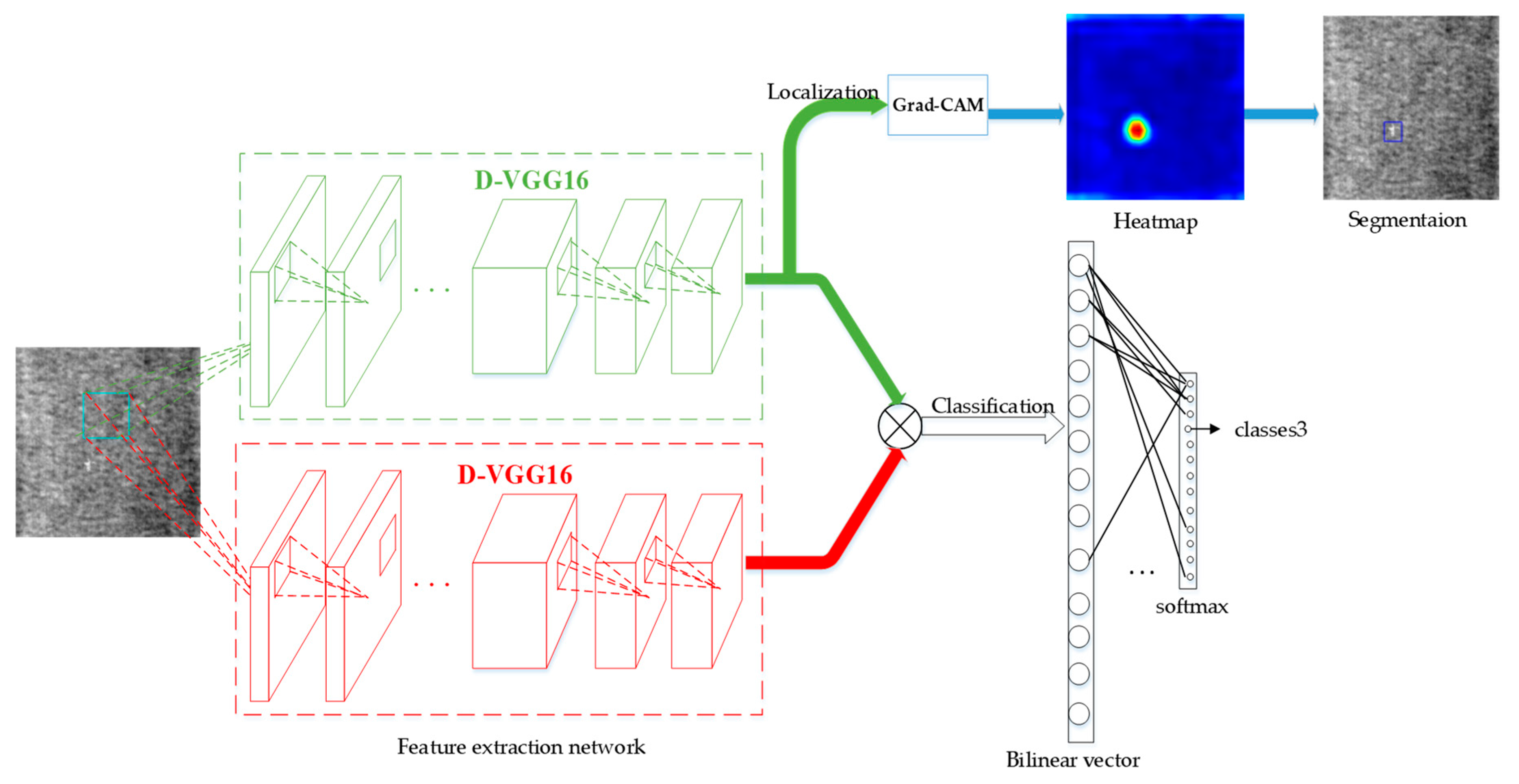
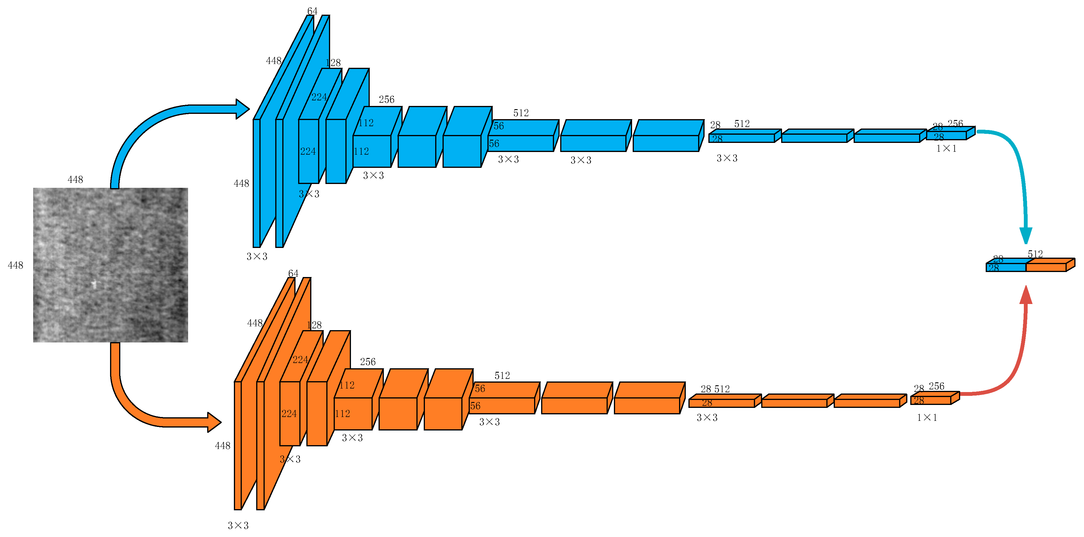
The whole process of defect classification is as follows: Two features that function from D-VGG16 are concatenated to get the bilinear vector, which is fed into the soft-max function to obtain the probability of the corresponding defects in the input image and realize the defect classification. The whole process is a typical bilinear model structure, and its core is D-VGG16 that is used as a feature function.

2.1.1. D-VGG16

Feature function, as a function extraction network of a bilinear model, plays an important role whatever for locating and classifying in the whole network. In this paper we used two fully symmetrical D-VGG16 that were based on VGG16, as a feature extraction network of a bilinear model were used, where the structure of the network is shown in Figure 2.
For the classification task using the Convolutional Neural Network (CNN), the simplest way to improve the accuracy of small sample training and avoid over-fitting is to reduce the feature map of the last layer of CNN without decreasing the receptive field of the network. However, this will inevitably influence the output features of the network, thereby limiting the expressive capability of the network. Given the considerations above, D-VGG16 is designed, as shown in Figure 2. As a 1 × 1 convolutional kernel with 256 channels, and this is used after the last convolution layer of the VGG16 network, and then the outputs of two such networks are concatenated to form D-VGG16. On the one hand, it can not only reduce the risk of an over-fitting of complex CNN for small samples training, but also maintain the diversity of the network output features, and the output features of two sub-networks can be conditioned on each other. The feature extraction network consists of two symmetrical D-VGG16, i.e., the two D-VGG16 are identical in architectures, so the entire network is composed of four VGG16 with exactly the same structure. The advantage of this design is that the global and local features of the image can be adequately extracted, making the network more easily able to detect the subtle features in the image. In training, each sub-network loaded the pre-training weights of VGG16 on ImageNet directly, and used transfer learning, which achieves the goal of small samples training.

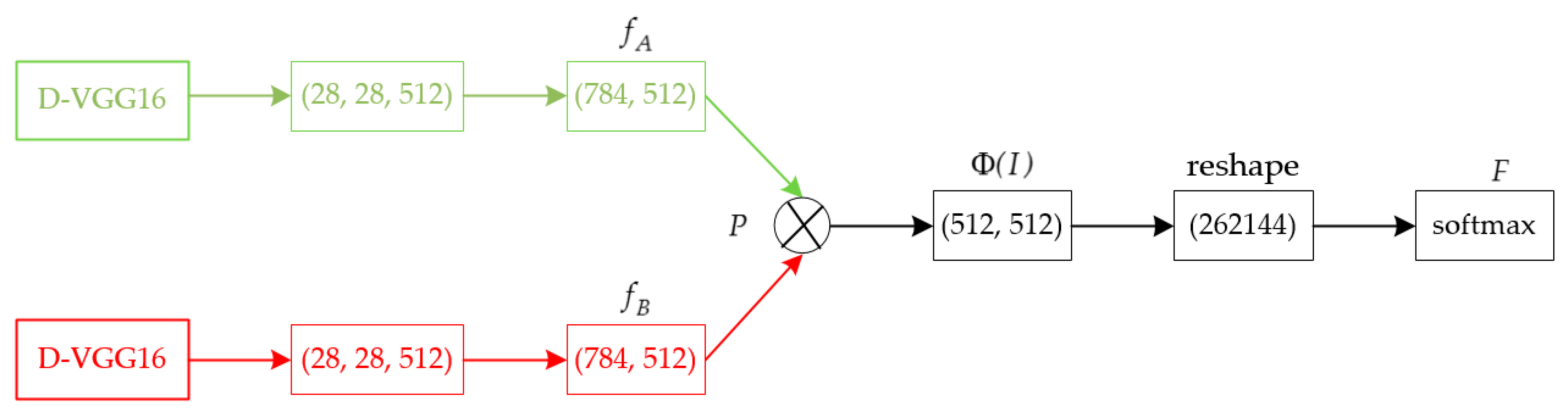
2.1.2. Bilinear Model

The bilinear model is composed of two-factors, and is mathematically separable, i.e., when one factor remains constant, its output is linear in any factor. A bilinear model B for defect classification consists of a quaternion function, as shown in Equation (1).
B = ( f A , f B , P , F )
where f A and f B are feature functions, D-VGG16 is used in this paper, P represents the pooling function, and F represents the classification function, which here refers to the soft-max classifier.
The output of the feature function, f A and f B , are combined at each position of the image I using the matrix inner product, as shown in Equation (2).
b i l i n e a r ( i , f A , f B ) = f A ( i ) T f B ( i )
where i I . The feature dimensions of f A and f B must be equal, and the value should be greater than 1 to represent various descriptors that can be written as bilinear models.
To obtain the descriptor of the image, the pooling function P aggregates the bilinear features across all of the locations in the image. The pooling function can use the weighted sum of all bilinear features of the image, i.e., the sum of all bilinear features, which was calculated as follows.
Φ ( I ) = i I b i l i n e a r ( i , f A , f B )
If the feature sizes of the f A and f B output are C × M and C × N respectively, then the size of the bilinear vector Φ ( I ) is M × N , and its corresponding class probability can be obtained by inputting the Φ ( I ) reshaped size M N × 1 into the classification function F . The data stream of this bilinear model is shown in the Figure 3.
From an intuitive point of view, the structure of the bilinear can make the output features of the feature extraction function, f A and f B , to be fine tuned on each other by considering all of their pairwise interactions similar to quadratic kernel expansion. Because the entire network is a directed acyclic graph, and parameters of the network can be trained by the gradient of back-propagating loss.

2.2. Defect Localization
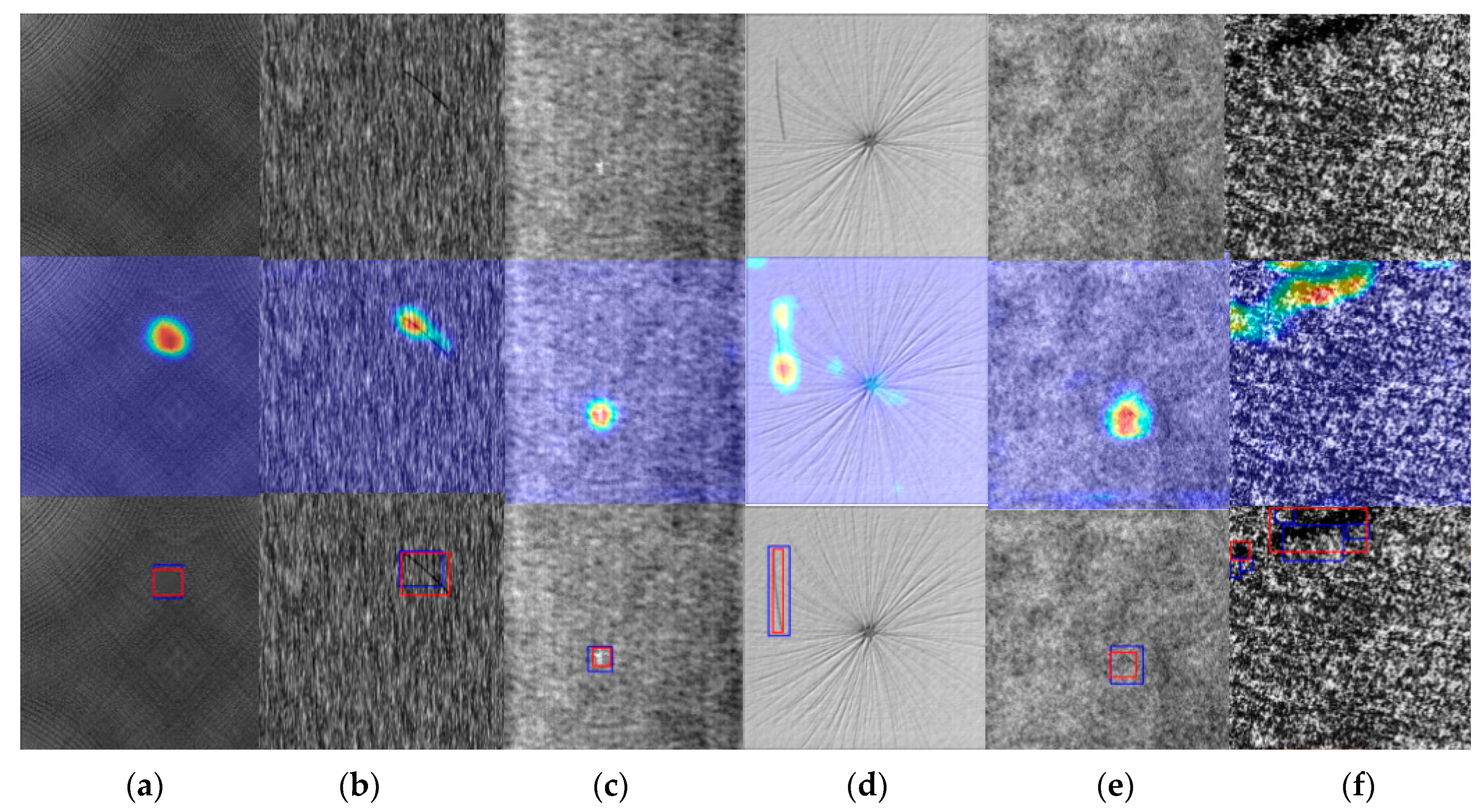
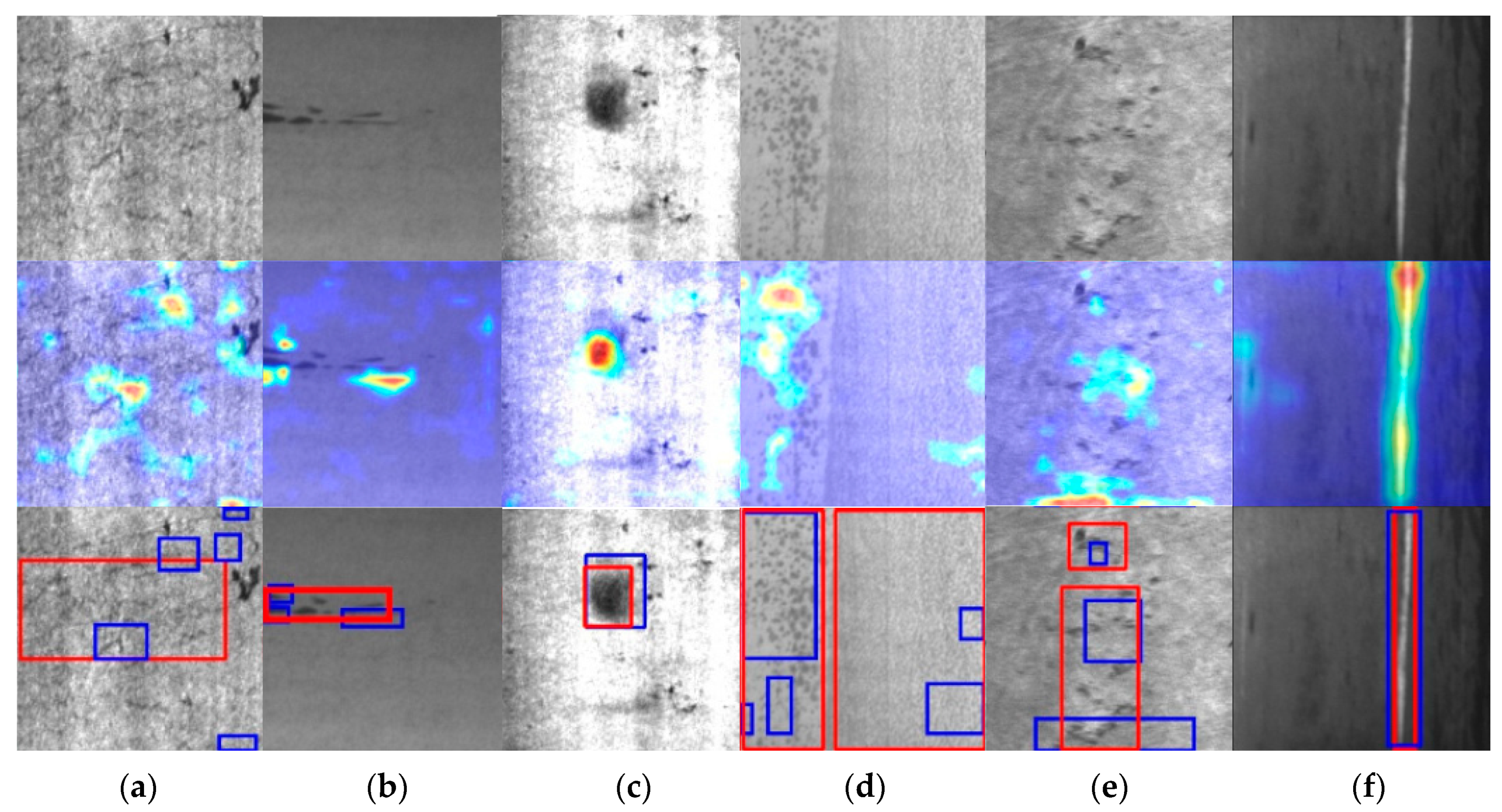
Defect localization of the input image enables the inspector to find and understand the specific location of the defect intuitively, and the implementation process is as follows: Firstly, the heat map of the original image is obtained by applying Gradient-weighted Class Activation Mapping (Grad-CAM) to one of the output features of D-VGG16, and then the corresponding defect location can be determined in the input image by a threshold segmentation to the heat map.

2.2.1. Grad-CAM

Although CNN has significant effects on image processing tasks for a long time, it has been a controversial method due to the poor interpretability of the CNN internal feature extraction, thus a new field, which is called the interpretable research of deep learning, appeared. Apart from that, Grad-CAM is a visualized method of the convolutional neural network, which can be used to visualize network category location results in the last level of the network’s convolutional layer.
In order to obtain a class activation map L G r a d C A M n , the score gradient y n A k of the class n is firstly calculated, in which A k represents the weight of the class n of the first k feature map, and y k represents the score of the category before the soft-max. Then the gradient of the global average pooling layer is used to obtain the importance α k n of the first k feature map for the category n .
α k n = 1 Z i j y n A i j k
where Z represents the size of the feature map and A i j k represents the activation value of the position in ( i , j ) the k first feature map. Finally, the weighted sum of the forward activation features is performed according to Formula (4), and a Grad-CAM of a given class can be obtained using a rectified linear unit (ReLU).
L G r a d C A M n = R e L U ( k α k n A k ) = max ( 0 , k α k n A k )
Grad-CAM can explain the feature extraction results of the network and enhance the trust of the network performance, which is particularly important to the training network of small samples, because the insufficient number of training samples may lead to an inadequately trained network, thus causing a problem that the judgments of the network for a particular class may not be based on the real discriminant region in the image, and this results in serious over-fitting. In addition, Grad-CAM is used in the defect detection network, which can automatically locate the defects of input images in the prediction stage only by image-level annotation in the training stage.
In this paper, the Grad-CAM of defective images are generated. As shown in Figure 1, the Grad-CAM highlights the defect regions.

2.2.2. Segmentation

The threshold segmentation is performed after the heat map of the input image obtained from Grad-CAM to locate the defect regions. Let f ( m , n ) represent the binarized image for the heat map, and f ( m , n ) is as shown in
f ( m , n ) = { 255 , if   f h m ( m , n ) σ 0 , otherwise
where f h m ( m , n ) indicates the heat map after graying, and σ is the threshold, respectively. In f ( m , n ) , pixels whose gray value is 255 indicate the defect region, and pixels whose gray value is 0 present the non-defective area. In order to get better localization results, it is significantly important to choose the threshold segmentation method for σ . Experiments show that different types of defects and defects distribution in the entire image can result in different methods of threshold segmentation. For images with defects of limited distribution and signal type, a simple fixed threshold segmentation can be used to obtain a better result. For images with defects of scattered distributions and variable types, the adaptive Otsu [25] algorithm can obtain satisfactory results.

3. Experiments

This section evaluates the performance of the surface defect detection method proposed in this paper on two public and two collected defect datasets in real industrial scenes. Firstly, the experimental hardware environment and training details are briefly explained. Secondly, the datasets used will be expounded. Then, the number of images for training and testing is interpreted. Finally, the proposed method is compared with the latest experimental method of each data set in four datasets, which highlight the effectiveness and universality of the proposed method on the task of surface defect detection.

3.1. Hardware Platform and Training Details

Experiments in this paper are implemented on a workstation with 64 GB memory, and we also used TITAN XP for acceleration. Similar to most deep convolutional neural networks, the back-propagation algorithm was used as the training rule, and we then minimized the loss function with respect to the network parameters using Adam [26]. The training of the whole network is carried out in an end-to-end way. The training and testing images of each dataset are labeled only with the image-level. Input images were resized to 448 × 448, with no preprocessing of the images except for normalization.
The training process of the whole network was in the form of transfer learning. Specific implementation steps were as follows: Firstly, the pre-training weights of VGG16 on ImageNet was loaded to initialize two D-VGG16, and only parameters other than VGG16 were trained. At this time, the learning rate was 0.001, the momentum was 0.9, and the batch size was 64, and a model with relatively low loss was trained. Then we load the weights of the last step to continue training the entire network. At this time, the learning rate was 0.00001, the momentum was 0.9, and the batch size was 16. In this schedule, a model with lower loss will be obtained by several iterations.

3.2. Datasets Description

The open datasets are DAGM_2007 [27] and hot-rolled strip [28], respectively. The collected datasets are the diode glass bulb surface defect dataset and the fluorescent magnetic powder surface defect dataset. These datasets cover texture defects, shape defects and color defects on the actual industrial product.

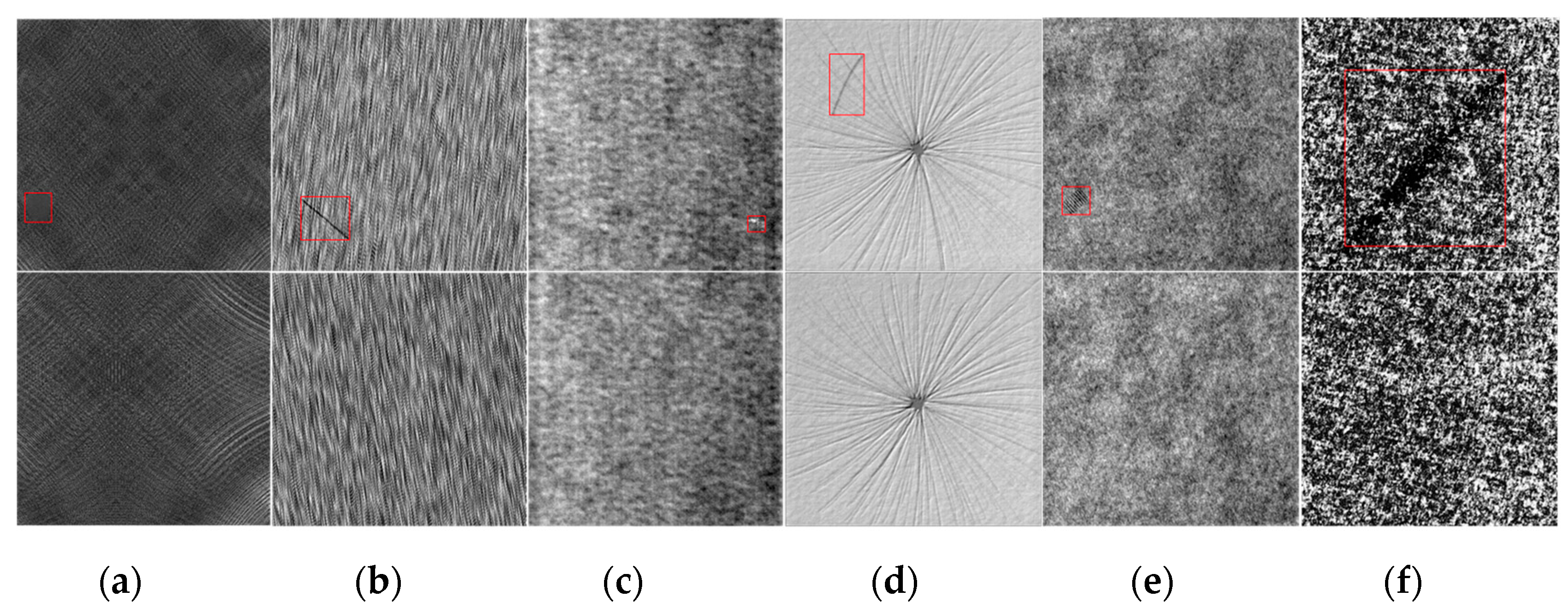
3.2.1. DAGM_2007 Defect Dataset

The first open dataset is the DAGM_2007 surface defect dataset, which is manually generated and can be used for surface defect detection. The dataset contains six types of surface defects with different textures, where in each of these defects has 1000 defect-free and 150 defective grayscale images, the size of the image is 512 × 512 pixels and the pixel precision is 8 bits. The ground truths of all defective images are provided in the dataset. Examples of defect images are shown in Figure 4.

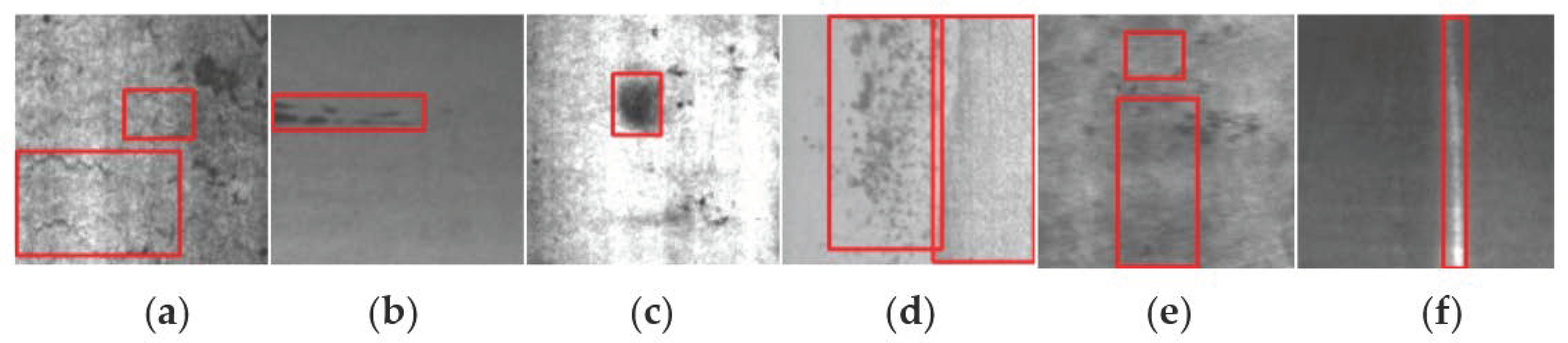
3.2.2. NEU Defect Dataset

NEU [24] is a surface defect dataset of hot-rolled steel strips. There are six types of defects, including crazing, inclusion, patches, pitted-surface, rolled-in scale and scratches. Examples of the defect images are shown in Figure 5. Each class of defect has 300 grayscale images, and the size of the image is 200 × 200 pixels, and the pixel precision is 24 bits. The labels of all of the images are provided in the dataset, but the ground-truth of the defective images is not provided.

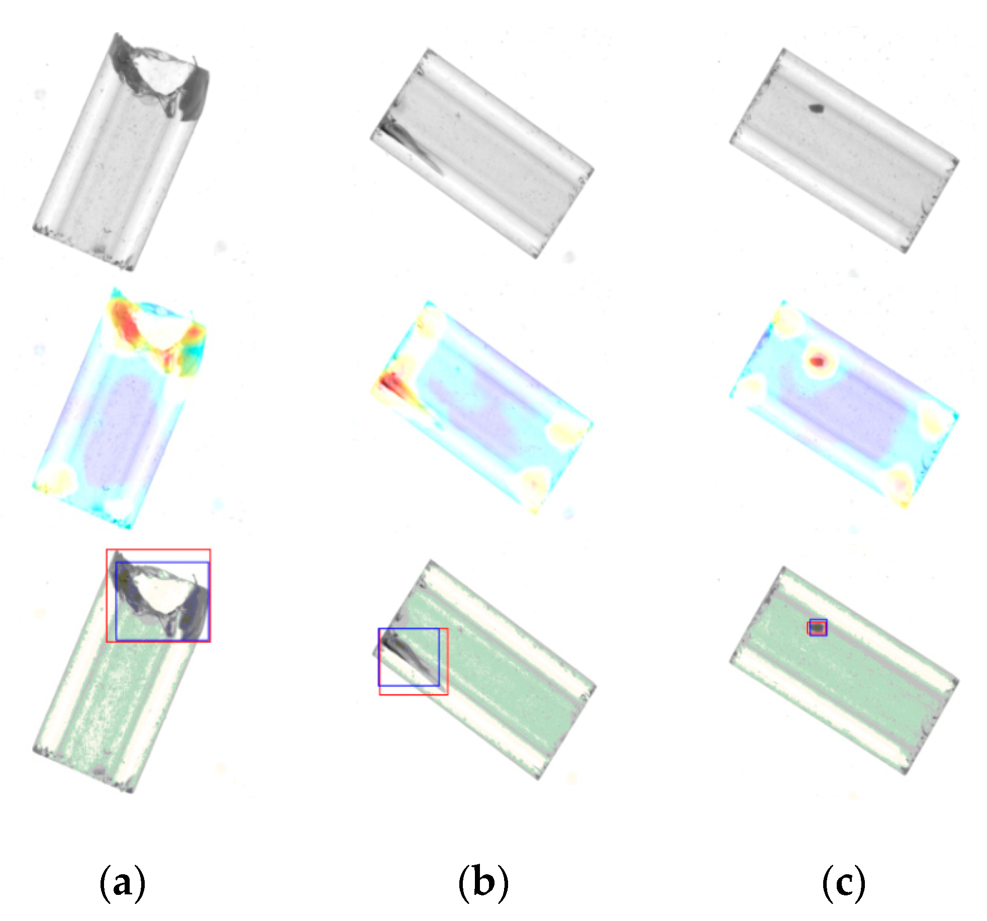
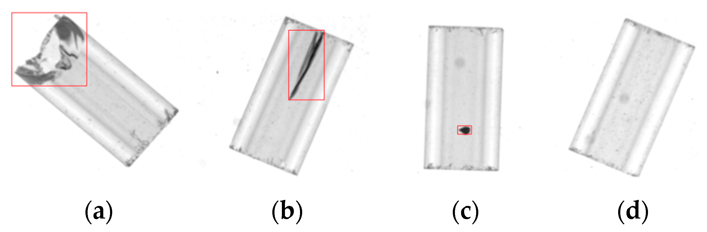
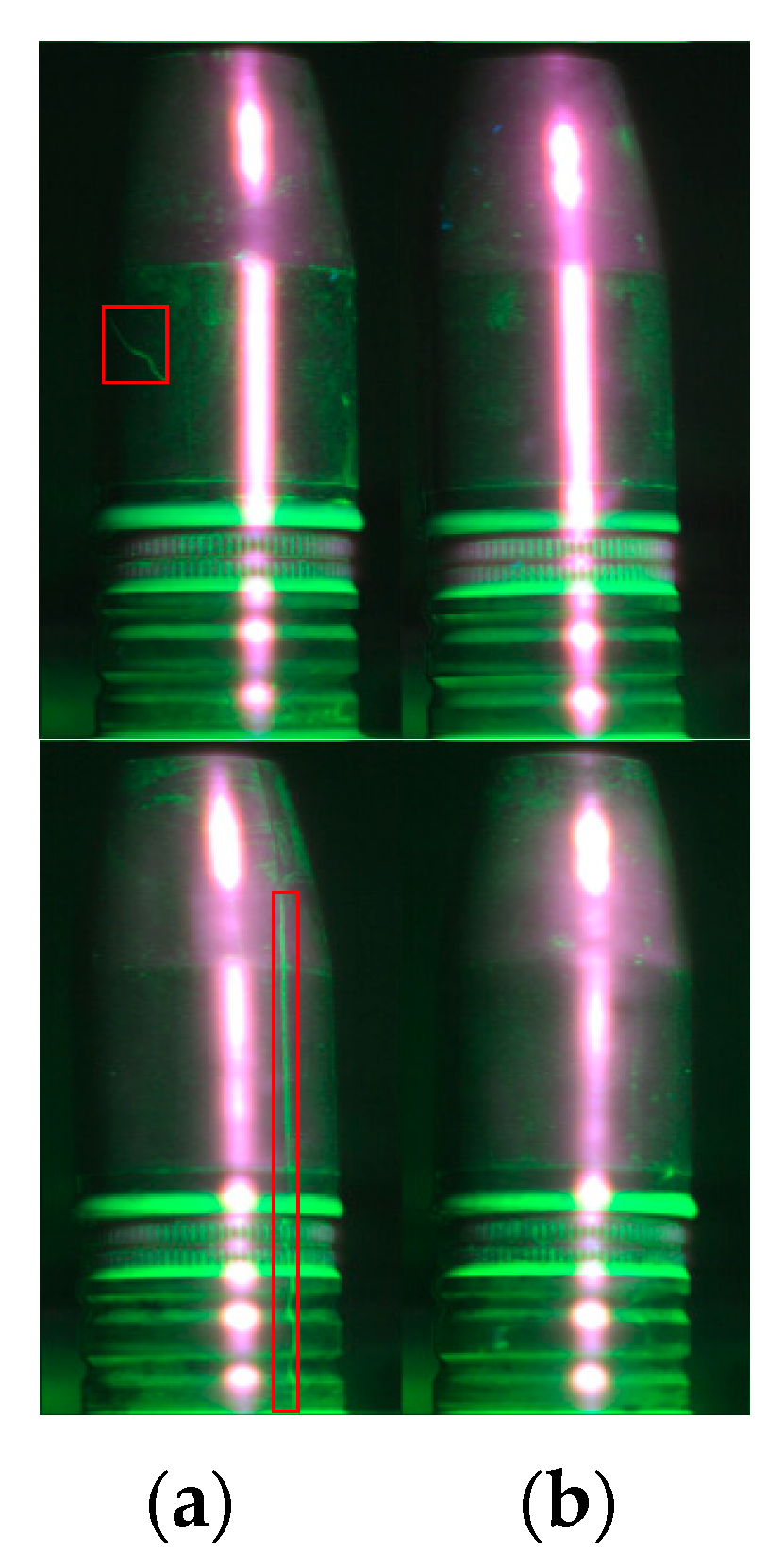
3.2.3. Diode Glass Bulb Surface Defect Dataset

The glass bulbs have been widely used as packaging material for diodes because of their heat resistance, damp-proof ability and high reliability. They play an important role in protecting the diode. In order to obtain surface images of the surface of the diode glass bulb, an image acquisition system consisting of an industrial camera with DAHENG IMAGING MER-131-75 GM/C-P, a telecentric lens with 1× magnification and a dark-field LED light source was used in the experiment. A total of 1730 color images were collected, of which 1020 were defective images, including 390 of shell wall damage, 360 breaks, 270 stains, and the size of the image is 661 × 601 pixels and the pixel precision is 8 bits. Examples of these defect images are shown in Figure 6.

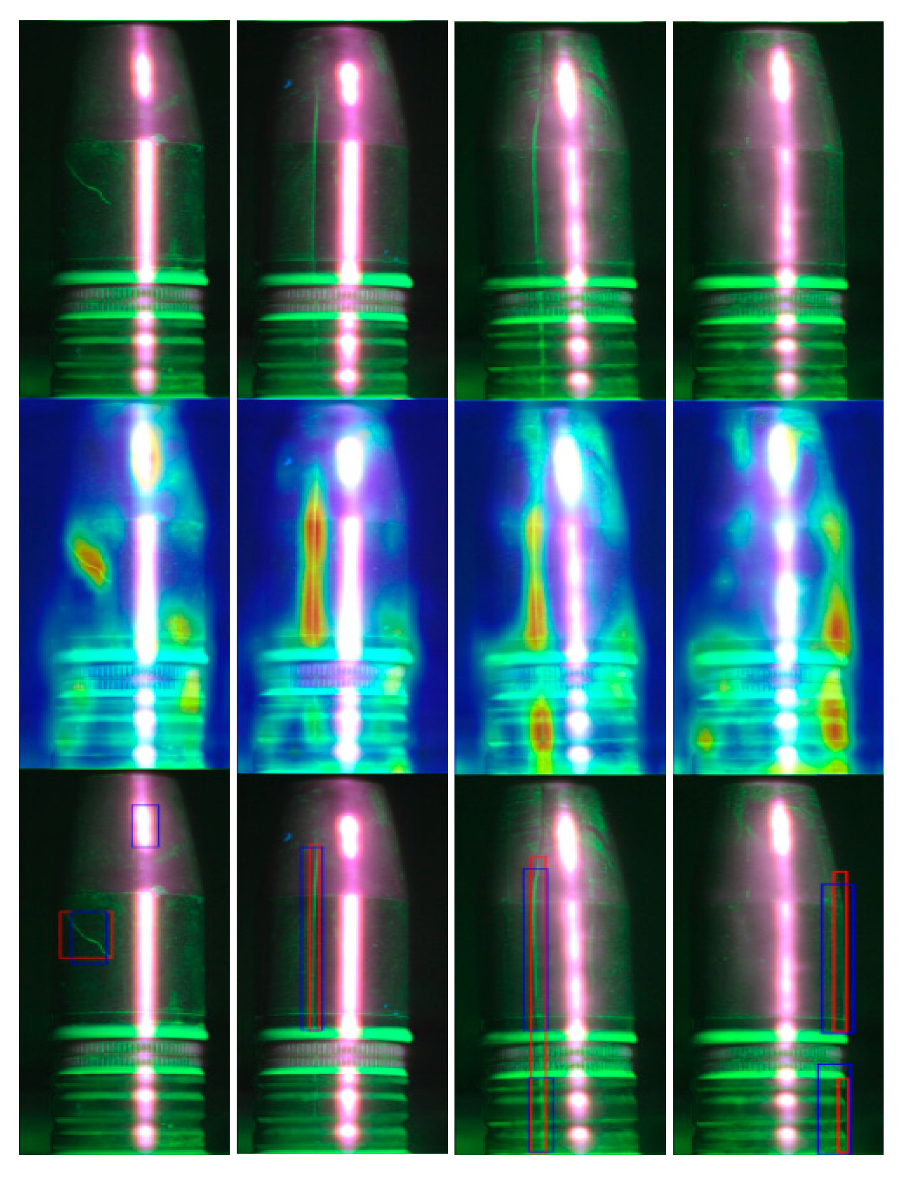
3.2.4. Fluorescent Magnetic Powder Surface Defect Dataset

Fluorescent magnetic powder nondestructive testing is a common method for the detection of any surface and near-surface defects of ferromagnetic materials such as aero-turbines [29], turbines [30], and train bearings [31] in the aerospace, military and civil industry. Its working principle is that after the ferromagnetic material work-piece is magnetized, the magnetic force line will be locally distorted when there are defects on the surface and near-surface of the work-piece. It leads to magnetic leakage, absorbing fluorescent magnetic particles suspended on the surface of the work-piece, and the forming of visible magnetic marks under ultraviolet light. In the experiment, the image acquisition system consisted of an industrial camera with XIMEA MQ042CG-CM, a fixed focus lens with a focal length of 6 mm and an ultraviolet light. The system was used to detect surface cracks of the ferromagnetic cylindrical work-pieces with the height of 100 mm and diameter of 45 mm, in which the width and height of the crack range from 0.3 mm to 1.0 mm and from 7 mm to 90 mm, respectively. The experiment collected 800 defects and 1000 defects-free color images, and the size of the image is 468 × 1324 pixels, and the pixel precision is 24 bits. Examples of defect images are shown in Figure 7.

3.3. Contrast Experiments

In order to test the performance of the proposed method in work-pieces surface defect detection, the proposed method is evaluated on two published and two collected work-pieces surface defect datasets. At present, most of the defect detection algorithms only aim at a specific category of defects; however, the surface defect detection method proposed in this paper is a kind of defect that can be applied to different types of work-pieces. It is unreasonable to apply a defect detection algorithm suitable for a specific category to other categories of defects and compare it with the method proposed in this paper.
Therefore, in each defect data set, not only GLCM + MLP [17], gcForest [32] and Bilinear Convolutional Neural Network (BCNN) are used to perform four kinds of generic surface defect detection algorithms, but also the open datasets will also be compared with the known latest experimental results on this dataset.

3.3.1. Open Datasets

Since the vast majority of the evaluations using the two datasets for performance evaluation had only the experimental results of average precision, and average precision is the main and most important performance indicator for the multi-category task, therefore only the average precision of the methods is compared on two open datasets.
(A) Localization and Classification Results of the DAGM_2007 Defect Dataset: For the DAGM_2007 dataset, the ratio of the training set to the test set is 1:1. Some experimental localization results of the proposed method running in the dataset are shown in Figure 8.
In the combination image of the original image and Grad-CAM, the red region represents the confidence level of the pixels that the network discriminates against. The deeper the color, the higher the confidence level of the pixels in the image. The dataset is compared with the results of surface defect detection algorithms proposed by Yu [33] and Zhao [34]. The experimental classification results are shown in Table 1.
As can be seen from Table 1, although high classification accuracy has been achieved on the DAGM_2007 surface defect data set at present, the proposed method can still further improve the classification accuracy on the data set and achieve the automatic location of defects at the same time.
(B) Localization and Classification Results of the NEU Defect Dataset: For the NEU surface defect dataset, a number of 150 images are randomly selected as the test set in each class of defects, and the remaining images are used as the training set. Some experimental localization results of the proposed method running in the dataset are shown in Figure 9.
Most images of the NEU defect dataset have multiple defects, and the texture of each type of defective image is different, which brings more challenges to automatic location. As shown in Figure 9, although the proposed method does not perform well in defect localization when applied to NEU datasets, it can extract specific pixel regions to identify a certain class of images. Using this dataset, the proposed method was compared with the algorithms proposed by BYEC [6], Song et al. [35] and Ren et al. [18]. To ensure the validity of the comparison results, the same training data generation method as the papers mentioned above is used. The experimental classification results are shown in Table 2.
As can be seen from Table 2, compared with the latest methods proposed by Sun and Ren, the proposed method has a higher detection accuracy in the NEU defect detection dataset.

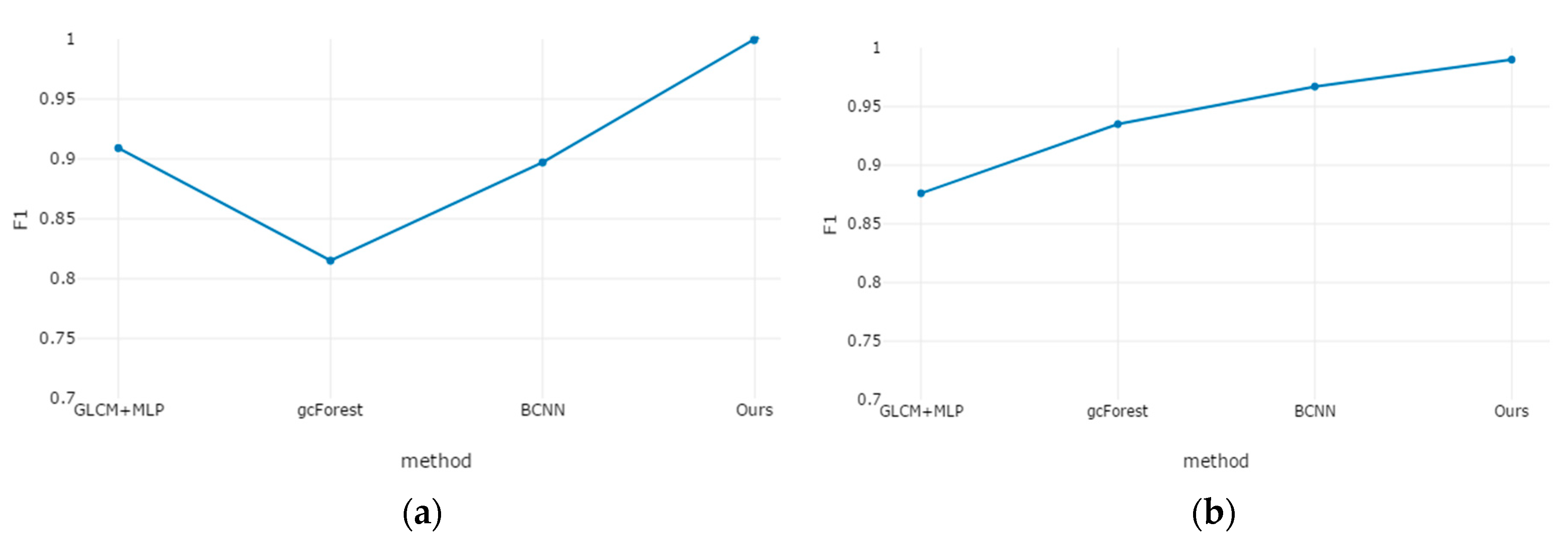
3.3.2. Real Collected Datasets

The two kinds of defect datasets collected contains defective and defect-free images, so they can be regarded as multi-classification or binary classification tasks.
(A) Localization and Classification Results of the Diode Glass Bulb Surface Defect Dataset: For the diode glass bulb surface defect dataset, the ratio of the training set and testing set images is 7:3. Some experimental localization results of defect detection on this dataset by the proposed method are shown in Figure 10.
There is no significant texture difference around different defect types in the diode glass bulb surface defect dataset, and shell wall damage is a typical shape defect. However, it can be found that the proposed method can accurately extract the key pixel regions that discriminate each type of defect, which can not only explain the reason why it can achieve a higher precision than other methods, but also obtain the better effect of localization. The comparative experiments on this dataset are shown in Table 3.
It can be seen from Table 3 that even in the work-piece surface defect detection task with few texture features, the proposed method has an advantage in detection accuracy compared with other algorithms.
(B) Localization and Classification Results of the Fluorescent Magnetic Powder Surface Defect Dataset: For this fluorescent magnetic powder surface defect dataset, the ratio of the training set and the testing set images is 7:3. The experimental localization results of the proposed method on this dataset are shown in Figure 11.
When the ultraviolet light is irradiated on the smooth iron work-piece, the surface of the magnetized work-piece will reflect the violet light emitted by the ultraviolet light due to the principle of light reflection. This phenomenon is particularly prominent on the cylindrical work-piece. Therefore, the defect image of the fluorescent magnetic powder obtained in the experiment has a bright purple reflective area in the center of the work-piece, which will cause a great interference to the detection of any defects. In the experiment, the original image is zoomed into a size of 448 × 448, with no pre-processing having been performed on the images except for normalization, and then the image is sent to the network for training and testing. As shown in Figure 11, it can be seen that the network can effectively eliminate interference in the reflective area and extract the defective area. The classification results of the comparative experiments on this dataset are shown in Table 4.
It can be seen from Table 4 that even if there is a task of defect detection with strong interference factors, the detection accuracy of the proposed method is still nearly 6% higher than that of BCNN.
(C) Evaluation of Binary Classification Performance: The above experiments have shown that the average precision of the proposed method on four datasets is higher than that of other methods. However, the detection rate of defects and the precision of non-defects are often emphasized in defect detection, and at this time, only the dataset is divided into defects and non-defects. TP and TN denote the number of true positives and true negatives respectively, FP and FN denote the number of false positives and false negatives, respectively. Then the definitions of the Precision Rate (PR), True Positive Rate (TPR), False Positive Rate (FPR) and False Negative Rate (FNR) are as follows.
P R = T P T P + F P
T P R = T P T P + F N
F P R = F P F P + T N
F N R = F N F N + T P
Results of the four methods PR, TPR, FPR and FNR on the diode glass bulb and fluorescent magnetic powder surface defect dataset are shown in Table 5.
Precision Rate and True Positive Rate are often a pair of contradiction measure, and generally speaking, when the Precision Rate is high, the True Positive Rate tends to be low, and the higher True Positive Rate, the lower the Precision Rate. Therefore, the Precision Rate and the True Positive Rate cannot accurately reflect the effectiveness of the detection method, but usually F 1 is used, which is defined as follows.
F 1 = 2 × P R × T P R P R + T P R
F 1 value of GLCM + MLP, gcForest, BCNN and the proposed method on the diode glass bulb surface defect dataset and fluorescent magnetic powder surface defect dataset are shown in Figure 12.
The results are shown in Figure 12. The proposed surface defect detection method achieves a higher F 1 among all of the methods. It outperforms both methods combining statistical features with machine learning (GLCM + MLP) and the generic deep learning method based on a Convolutional Neural Network (BCNN).
There are many kinds of defects in actual industrial production, and one method which works well in a specific category is usually not applicable to the other types of defects. Experimental results show that the surface defect detection method proposed in this paper demonstrates excellent detection performance in surface defects with features of texture, shape and color. Furthermore, it can simultaneously realize an automatic localization and classification of defects. In the prediction phase, it takes an average of 0.292 s to a localization and classification of defects for an image at the same time.

4. Conclusions

The conclusions from the work are presented as follows.
  • A generic method of automated surface defect detection based on a bilinear model is proposed. Firstly, as a feature extraction network of the bilinear model, D-VGG16, which consists of two completely symmetric VGG16, is designed, and the features extracted from the bilinear model are output to the soft-max function to realize the automatic classification of defects. Then the heat map of the original image is obtained through applying Grad-CAM to one of the output features in D-VGG16. Finally, the defects in the input image can be located automatically after processing the heat map with a threshold segmentation algorithm.
  • The training of the proposed method is carried out in a small sample, end-to-end, and in a weakly-supervised way. Even though the number of training images used in the experiments were no more than 1300, over-fitting did not occur during the training process of all the datasets, and the surface defects can be automatically located using only training images labeled at image-level.
  • The experiments has been performed on four datasets with different defective features. This shows that the proposed method can be effectively applied to surface defect detection scenarios with texture, color and shape features, even a diode glass bulb surface defect dataset with complex texture and the fluorescent magnetic powder surface defect dataset with strong interference factors. The overall performance of the proposed method is superior to other methods.
The proposed method has certain limitations for automatic localization in the datasets with complex textures. Since the whole network is composed of four VGG16, and the Grad-CAM used in automatic localization is time-consuming, it takes a long time to detect and locate defect in the testing stage. Future work will focus on solving the above effect of automatic location and real-time performance of the method in this paper.

Author Contributions

F.Z. designed the algorithm, performed the experiments and wrote the paper. G.L. modified the paper. F.X. and. H.D. supervised the research.

Funding

This work was supported by National Natural Science Foundation of China (Grant Nos. 11602292, 61701421, 61601381).

Conflicts of Interest

The authors declare no conflict of interest.

References

  1. Shafarenko, L.; Petrou, M.; Kittler, J. Automatic watershed segmentation of randomly textured color images. IEEE Trans. Image Process. 1997, 6, 1530–1544. [Google Scholar] [CrossRef] [PubMed]
  2. Ojala, T.; Pietikäinen, M.; Mäenpää, T. Multiresolution gray-scale and rotation invariant texture classification with local binary patterns. IEEE Trans. Pattern Anal. Mach. Intell. 2002, 7, 971–987. [Google Scholar] [CrossRef]
  3. Wen, W.; Xia, A. Verifying edges for visual inspection purposes. Pattern Recognit. Lett. 1999, 20, 315–328. [Google Scholar] [CrossRef]
  4. Zhou, P.; Xu, K.; Liu, S. Surface defect recognition for metals based on feature fusion of shearlets and wavelets. Chin. J. Mech. Eng. 2015, 51, 98–103. [Google Scholar] [CrossRef]
  5. Ghorai, S.; Mukherjee, A.; Gangadaran, M.; Dutta, P.K. Automatic defect detection on hot-rolled flat steel products. IEEE Trans. Instrum. Meas. 2012, 62, 612–621. [Google Scholar] [CrossRef]
  6. Xiao, M.; Jiang, M.; Li, G.; Xie, L.; Yi, L. An evolutionary classifier for steel surface defects with small sample set. EURASIP J. Image Video Process. 2017, 2017, 48. [Google Scholar] [CrossRef]
  7. Santoyo, E.A.R.; Lopez, A.V.; Serrato, R.B.; Garcia, J.A.J.; Esquivias, M.T.; Fernandez, V.F. Reconocimiento de patrones y evaluación del daño generado en aceros de baja aleación a partir del procesamiento digital de imágenes e inteligencia artificial. DYNA Ing. Ind. 2019, 94, 357. [Google Scholar]
  8. Li, Y.; Chen, X.; Zhu, Z.; Xie, L.; Huang, G.; Du, D.; Wang, X. Attention-guided unified network for panoptic segmentation. In Proceedings of the IEEE Conference on Computer Vision and Pattern Recognition (CVPR), Long Beach, CA, USA, 16–20 June 2019. [Google Scholar]
  9. Feng, W.; Hu, Z.; Wu, W.; Yan, J.; Ouyang, W. Multi-Object Tracking with Multiple Cues and Switcher-Aware Classification. arXiv 2019, arXiv:1901.06129. [Google Scholar]
  10. Lin, H.; Li, B.; Wang, X.; Shu, Y.; Niu, S. Automated defect inspection of LED chip using deep convolutional neural network. J. Intell. Manuf. 2018, 30, 2525–2534. [Google Scholar] [CrossRef]
  11. Zhou, B.; Khosla, A.; Lapedriza, A.; Oliva, A.; Torralba, A. Learning deep features for discriminative localization. In Proceedings of the IEEE conference on Computer Vision and Pattern Recognition, Las Vegas, NV, USA, 27–30 June 2016. [Google Scholar]
  12. Tao, X.; Zhang, D.; Ma, W.; Liu, X.; Xu, D. Automatic metallic surface defect detection and recognition with convolutional neural networks. Appl. Sci.-Basel 2018, 8, 1575. [Google Scholar] [CrossRef]
  13. Di, H.; Ke, X.; Peng, Z.; Dongdong, Z. Surface defect classification of steels with a new semi-supervised learning method. Opt. Lasers Eng. 2019, 117, 40–48. [Google Scholar] [CrossRef]
  14. Lin, W.-Y.; Lin, C.-Y.; Chen, G.-S.; Hsu, C.-Y. Steel Surface Defects Detection Based on Deep Learning. In Proceedings of the International Conference on Applied Human Factors and Ergonomics (AHFE), Orlando, FL, USA, 22–26 July 2018. [Google Scholar]
  15. Ren, S.; He, K.; Girshick, R.; Sun, J. Faster r-cnn: Towards real-time object detection with region proposal networks. In Proceedings of the Advances in Neural Information Processing Systems, Montreal, QC, Canada, 7–12 December 2015; pp. 91–99. [Google Scholar]
  16. Liu, W.; Anguelov, D.; Erhan, D.; Szegedy, C.; Reed, S.; Fu, C.-Y.; Berg, A.C. Ssd: Single shot multibox detector. In Proceedings of the European Conference on Computer Vision (ECCV), Amsterdam, The Netherlands, 8–16 October 2016. [Google Scholar]
  17. Cha, Y.J.; Choi, W.; Suh, G.; Mahmoudkhani, S.; Büyüköztürk, O. Autonomous structural visual inspection using region-based deep learning for detecting multiple damage types. Comput. Aided Civ. Infrastruct. Eng. 2018, 33, 731–747. [Google Scholar] [CrossRef]
  18. Ren, R.; Hung, T.; Tan, K.C. A generic deep-learning-based approach for automated surface inspection. IEEE Trans. Cybern. 2017, 48, 929–940. [Google Scholar] [CrossRef] [PubMed]
  19. Lin, M.; Chen, Q.; Yan, S. Network in network. In Proceedings of the International Conference on Learning Representations (ICLR), Scottsdale, AZ, USA, 2–4 May 2013. [Google Scholar]
  20. Selvaraju, R.R.; Cogswell, M.; Das, A.; Vedantam, R.; Parikh, D.; Batra, D. Grad-cam: Visual explanations from deep networks via gradient-based localization. In Proceedings of the IEEE International Conference on Computer Vision (ICCV), Venice, Italy, 22–29 October 2017. [Google Scholar]
  21. Simonyan, K.; Zisserman, A. Very deep convolutional networks for large-scale image recognition. In Proceedings of the International Conference on Learning Representations, Banff, AB, Canada, 14–16 April 2014. [Google Scholar]
  22. Lin, T.-Y.; RoyChowdhury, A.; Maji, S. Bilinear cnn models for fine-grained visual recognition. In Proceedings of the IEEE International Conference on Computer Vision, Santiago, Chile, 7–13 December 2015. [Google Scholar]
  23. Deng, J.; Dong, W.; Socher, R.; Li, L.-J.; Li, K.; Li, F.-F. Imagenet: A large-scale hierarchical image database. In Proceedings of the 2009 IEEE Conference on Computer Vision and Pattern Recognition, Miami, FL, USA, 20–25 June 2009. [Google Scholar]
  24. Yosinski, J.; Clune, J.; Bengio, Y.; Lipson, H. How transferable are features in deep neural networks? In Proceedings of the Advances in Neural Information Processing Systems, Montreal, QC, Canada, 8–13 December 2014; pp. 3320–3328. [Google Scholar]
  25. Ostu, N. A threshold selection method from gray-histogram. IEEE Trans. Syst. Man Cybern. 1975, 9, 62–66. [Google Scholar]
  26. Kingma, D.P.; Ba, J. Adam: A method for stochastic optimization. In Proceedings of the International Conference on Learning Representations, Banff, AB, Canada, 14–16 April 2014. [Google Scholar]
  27. DAGM 2007 Datasets. Available online: https://hci.iwr.uni-heidelberg.de/node/3616 (accessed on 29 July 2019).
  28. Song, K.; Yan, Y. A noise robust method based on completed local binary patterns for hot-rolled steel strip surface defects. Appl. Surf. Sci. 2013, 285, 858–864. [Google Scholar] [CrossRef]
  29. Coro, A.; Abasolo, M.; Aguirrebeitia, J.; López de Lacalle, L. Inspection scheduling based on reliability updating of gas turbine welded structures. Adv. Mech. Eng. 2019, 11, 1687814018819285. [Google Scholar] [CrossRef]
  30. Artetxe, E.; Olvera, D.; de Lacalle, L.N.L.; Campa, F.J.; Olvera, D.; Lamikiz, A. Solid subtraction model for the surface topography prediction in flank milling of thin-walled integral blade rotors (IBRs). Int. J. Adv. Manuf. Technol. 2017, 90, 741–752. [Google Scholar] [CrossRef]
  31. Zhao, M.; Lin, J.; Miao, Y.; Xu, X.J.M. Detection and recovery of fault impulses via improved harmonic product spectrum and its application in defect size estimation of train bearings. Measurement 2016, 91, 421–439. [Google Scholar] [CrossRef]
  32. Zhou, Z.-H.; Feng, J. Deep forest: Towards an alternative to deep neural networks. In Proceedings of the International Joint Conference on Artificial Intelligence (IJCAI), Melbourne, Australia, 19–25 August 2017. [Google Scholar]
  33. Yu, Z.; Wu, X.; Gu, X. Fully convolutional networks for surface defect inspection in industrial environment. In Proceedings of the International Conference on Computer Vision Systems (ICVS), Venice, Italy, 22–29 October 2017. [Google Scholar]
  34. Zhao, Z.; Li, B.; Dong, R.; Zhao, P. A Surface Defect Detection Method Based on Positive Samples. In Proceedings of the Pacific Rim International Conference on Artificial Intelligence (PRICAI), Nanjing, China, 28–31 August 2018. [Google Scholar]
  35. Song, K.; Hu, S.; Yan, Y. Automatic recognition of surface defects on hot-rolled steel strip using scattering convolution network. J. Comput. Inf. Syst. 2014, 10, 3049–3055. [Google Scholar]
Figure 1. Network overall structure.
Applsci 09 03159 g001
Figure 2. Double-Visual Geometry Group16 (D-VGG16) network structure. Feature maps with the same shape have the same width, height, number of channels and convolutional kernel.
Applsci 09 03159 g002
Figure 3. Data stream of the bilinear model.
Applsci 09 03159 g003
Figure 4. Examples of the DAGM_2007 defect dataset. Each column represents a type of defect, and the defect areas are labeled by the red bounding boxes. (a) classes1; (b) classes2; (c) classes3; (d) classes4; (e) classses5; (f) classes6.
Applsci 09 03159 g004
Figure 5. Examples of the NEU defect dataset. Each column represents a type of defect, and the defect areas are labeled by the red bounding boxes. (a) crazing; (b) inclusion; (c) patches; (d) pitted-surface; (e) rolled-in-scale; (f) scratches.
Applsci 09 03159 g005
Figure 6. Examples of the diode glass bulb surface defect dataset, and the defect areas are labeled by the red bounding boxes. (a) break; (b) shell wall damage; (c) stain; (d) good.
Applsci 09 03159 g006
Figure 7. Examples of the fluorescent magnetic powder surface defects dataset. The defect areas are labeled by the red bounding boxes. (a) bad; (b) good.
Applsci 09 03159 g007
Figure 8. Examples of localization on DAGM_2007 defect dataset. From top to bottom are the original image, the combination of the original image and the heat map, and the location results of the defects. The Ground-Truth of the defect is marked with the red bounding boxes, while the localization results of the proposed method is marked with the blue bounding boxes. (a) classes1; (b) classes2; (c) classes3; (d) classes4; (e) classses5; (f) classes6.
Applsci 09 03159 g008
Figure 9. Localization results of the proposed method on the NEU defect dataset. From top to bottom are the original image, the combination of the original image and the heat map, and the location results of the defects. The Ground-Truth of the defect is marked with the red bounding boxes, and the localization results of the proposed method is marked with the blue bounding boxes. (a) crazing; (b) inclusion; (c) patches; (d) pitted-surface; (e) rolled-in-scale; (f) scratches.
Applsci 09 03159 g009
Figure 10. Examples of localization on the diode glass bulb surface defect dataset. From top to bottom are the original image, the combination of the original image and the heat map, and the location results of these defects. The Ground-Truth of the defect is marked with the red bounding boxes, while the localization results of the proposed method is marked with the blue bounding boxes. (a) break; (b) shell wall damage; (c) stain.
Applsci 09 03159 g010
Figure 11. Localization results of the proposed method on the fluorescent magnetic powder surface defect dataset. From top to bottom are the original image, the combination of the original image and the heat map, and the location results of these defects. The Ground-Truth of the defect is marked with the red bounding boxes, and the localization result of the proposed method is marked with the blue bounding boxes.
Applsci 09 03159 g011
Figure 12. Comparison of F 1 curve obtained from four methods. (a) Diode glass bulb surface defect dataset; (b) Magnetic powder surface defect dataset.
Applsci 09 03159 g012
Table 1. Comparison of results on DAGM_2007 surface defect dataset.
MethodAverage Precision
GLCM + MLP81.68%
gcForest86.67%
BCNN95.57%
FCN [33]98.35%
Zhao [34]98.53%
Ours99.49%
Table 2. Comparison of results on NEU surface defect dataset.
MethodAverage Precision
GLCM + MLP98.61%
gcForest61.56%
BCNN98.56%
BYEC96.30%
Song [35]98.60%
Ren [18]99.21%
Ours99.44%
Table 3. Comparison of results on the diode glass bulb surface defect dataset.
MethodAverage Precision
GLCM + MLP91.32%
gcForest85.25%
BCNN91.80%
Ours99.87%
Table 4. Comparison of results on fluorescent magnetic powder surface defect dataset.
MethodAverage Precision
GLCM + MLP90.56%
gcForest92.59%
BCNN93.33%
Ours99.13%
Table 5. Results of the four methods PR, TPR, FPR and FNR on the diode glass bulb and fluorescent magnetic powder surface defect datasets.
DatasetDiode Glass Bulb Surface Defect DatasetFluorescent Magnetic Powder Surface Defect Dataset
Method PRTPRFPRFNRPRTPRFPRFNR
GLCM + MLP93.86%88.21%6.14%11.79%85.71%89.55%14.28%10.45%
grForest83.19%79.84%16.81%20.16%95%91.94%5%8.06%
BCNN81.25%100%18.75%0%99.65%94%0.35%6%
Ours100%100%0%0%98.36%99.67%1.64%0.33%

