A Simplified Thermal Model and Online Temperature Estimation Method of Permanent Magnet Synchronous Motors

Abstract

Monitoring critical temperatures in permanent magnet synchronous motors is crucial for improving working reliability. Aiming at resolving the difficulty in online temperature estimation, an accurate and simple five-node lumped parameter thermal network (LPTN) is proposed and the mathematical model of the LPTN is built. Both radial and axial heat transfer paths inside the motor are considered to model the complete thermal circuit. In addition, an innovative parameter identification method based on multiple linear regression is applied to identify the parameters of the LPTN model. The parameters in the state equation are identified instead of the data of the motor, which are strongly dependent on the material and geometrical parameters. Finally, an open-loop estimation scheme based on the state equation and Kalman filter algorithm is adopted to predict the motor temperature online. The model performances are validated by extensive experiments under varying speed and torque conditions in terms of the accuracy and robustness. The results indicate that the temperature estimation error is within the range of ±5 °C in most cases and the proposed model can quickly follow the load variation. Besides, the online temperature estimation scheme and parameter identification method are easy and convenient to implement in an embedded system, which is feasible in automobile applications.

1. Introduction

Permanent magnet synchronous motors (PMSMs) have been widely used in automotive traction drives due to their high performance, efficiency, and power density [1,2,3]. PMSMs should be operated within a specified range of temperature rise without any risk of demagnetization and stator winding failure [4,5,6]. So, it is essentially important to accurately predict and monitor motor temperatures [7,8].

Currently, there are mainly four methods for the thermal analysis of motors, i.e., finite element method (FEM), estimation method based on the rotor flux, estimation method based on the rotor high frequency impedance, and lumped parameter thermal networks (LPTNs). FEM can simulate the electromagnetic field and temperature field of the motor by means of multi-physics coupling. A combination of thermal and electromagnetic analysis was applied to analyze the behavior of the motor through FEM [9,10], and the minimum ferromagnetic analysis was used to determine the parameters of the equivalent circuit of the induction motor [10]. Reigosa proposed the rotor temperature estimation method based on rotor flux linkage. This method is not computationally intensive and simple to conduct [11]. The rotor temperature estimation method based on high frequency injection was proposed in [12,13,14]. The temperature of the permanent magnet not only affected the magnetic flux of the permanent magnet but also changed the transient resistance of the rotor. If the transient resistance of the rotor can be obtained, the temperature of the rotor can be obtained indirectly. Therefore, when the rotor transient impedance was observed under the condition of high-frequency voltage, the rotor temperature information can be obtained by the relationship between the transient resistance and the temperature [12].

However, the above-mentioned methods have some drawbacks. FEM has high estimation accuracy, but this method depends on the motor geometry, material properties, and boundary conditions, resulting in complex calculation and longer computing times. Thus, it can only be used for off-line analysis in the motor temperature field. Although the motor rotor temperature estimation algorithm based on rotor flux linkage is simple and easy to conduct, it is only able to predict the rotor temperature. In addition, the estimation accuracy depends on the observation accuracy of the rotor flux linkage, and the change of the flux linkage caused by temperature is not completely linear. Therefore, it is difficult to obtain a more accurate estimation of the rotor temperature. Compared with the method based on the rotor flux observation, the advantage of the approach based on the high frequency injection is that the change in rotor transient impedance is easier to detect. However, the injected high frequency signal may bring additional rotor loss, causing an increase in temperature.

A suitable alternative to monitor motor temperature is lumped parameter thermal networks (LPTNs). This thermal network model is a simplification of the motor physical model and its structure has obvious physical meanings, which can be applied to estimate the motor temperature online [15,16,17]. Three different methods for establishing LPTN have been proposed according to the number of the thermal model nodes [18]: Dark gray-box LPTN, light gray-box LPTN, and white-box LPTN. Dark gray-box LPTNs are strongly abstracted from the complicated motor thermal structure. In general, two to five nodes are selected to predict the temperature in the most dominant hear paths. The parameter identification of the thermal model is realized based on the experimental data from the sensor [18,19,20,21,22,23,24,25]. Compared with the modelling of the dark gray-box LPTN, the light gray-box LPTNs take more heat paths into consideration. More thermal nodes (5–15 nodes) are set up to design the LPTN based on heat transfer theory [26,27]. A major drawback of this approach originates from the dependence of the material and geometrical parameter of the motor with respect to the model parameter calculation. White-box LPTNs are composed of several sub-nodes, which more accurately reflect the real thermal distribution in the motor. However, considerable nodes require more computation cost when adopting this method [28,29].

In the case of the electric vehicle (EV) application, the dark gray-box LPTN has drawn more attention, since high demands are placed on cost and real-time computation in this industry. In addition, full material and geometric information of the motor is hard to access. The establishment of light gray-box LPTNs and white-box LPTNs is based on heat transfer theory. The accuracy of this method is difficult to guarantee due to the high dependency of the motor geometry model and the heat transfer characteristic of the material. Besides, the large differential-algebraic-equation system leads to complex calculation, which is not suitable for online temperature estimation. Thus, dark gray-box LPTNs are suitable to predict the temperature distribution in the PMSM of EVs. Three-node thermal models for accurate temperature estimation in permanent magnets, windings, and end windings are introduced in [20,21,23]. This modeling behavior is under some assumptions that the temperature distribution is homogeneous among each motor component and the other heat paths are ignored. In order to monitor the temperature of critical parts accurately, these components should be divided into several parts to get the precise heat distribution. With respect to the crucial part, the motor stator, Wallscheid divided the stator node into three nodes, i.e., the stator yoke, stator teeth, and stator winding [18]. The model robustness and accuracy were validated with a maximum temperature error of 8 $℃$. However, the above-mentioned studies only considered heat transfer in the radial direction neglecting the axial heat flow, and thus the real thermal flow among the PMSM cannot be reflected. However, the compromise between the precision and size of the reduced model must be made when employing the dark gray-box LPTN. Therefore, a simplified five-node thermal model is proposed in this paper considering both the real thermal flow and simplification of the model. We consider both the radial and axial heat transfer paths inside the motor and try to set up minimum thermal nodes to simulate the complete thermal circuit.

In the existing literature, the specific parameters in the thermal model are identified instead of the data in the state equation applying a complex scheme [19,20], which requires more computational resources and processing time. Thus, considering the good linear relationship of the state equation for the simplified thermal model, the multiple linear regression algorithm method is proposed in this paper to identify the thermal model parameter. This method does not depend on the structural parameters of the motor. It is unnecessary to identify each specific parameter in the thermal model, and only the parameters in the state equation need to be identified.

In conclusion, the proposed five-node LPTN and parameter identification method are aimed at solving temperature estimation problems in automobile applications. Since the cost pressure and demand on real-time execution is very high in this industry, the proposed algorithm should not be complicated when applied in an embedded system, which has to deal with multiple tasks in the meantime. Under consideration of the specific application in the automobile industry, the proposed scheme is easy and convenient to implement. In addition, the temperature accuracy proves the effectiveness of the proposed method.

This paper is organized as follows: In Section 2, the LPTNs of PMSMs based on the principle of heat transfer are simplified and five-node LPTNs are proposed; in Section 3, motor loss is calculated; in Section 4, the multiple linear regression method is employed to identify the thermal model parameters; in Section 5, the open-loop estimation scheme based on the equation of state and the Kalman filter algorithm are applied to online estimate the temperature of three critical parts, i.e., rotor, stator, and end cap. In Section 6, the model performances are validated by the experiment. Finally, the conclusions of this study are presented in Section 7.

2. Proposed Thermal Model

2.1. Simplified Lumped Parameter Thermal Model

Mellor [30] analyzed the structure of a fully enclosed air-cooled induction motor and proposed a 10-node LPTN-based on heat transfer theory, as shown in Figure 1. According to the motor structure, this model is divided into 10 nodes: The casing, stator core, stator teeth, stator coil, air gap, end winding, end cover air gap, rotor coil, rotor core, and shaft. It reflects the heat transfer process inside the motor objectively and is therefore widely applied to offline temperature analysis of motors.

However, the accuracy of the thermal model based on heat transfer theory is difficult to guarantee. The reasons are listed as follows:

• Ignoring the contact resistance: In LPTN, the internal thermal resistance of the solid is mainly considered, and the contact thermal resistance between the solids is neglected. In fact, due to the influence of factors, such as installation, this part of the thermal resistance has a great impact on the radial heat flow.
• High dependence on the accuracy of the motor geometry model and the heat transfer characteristics of the material: In order to obtain an accurate motor model, a considerable number of motor dimensions and material-related parameters are required. In actual engineering practice, full material and geometric information is not available.
• The fluid model accuracy is not ideal: The model established for the internal air of the motor is based on the empirical formula of heat transfer theory. However, these formulas are sensitive to the size and shape of the air gap.
• Complex calculation, not suitable for online estimation: It can be found that the model order is too high due to the modeling of each part of the motor, leading to the large differential-algebraic-equation system.

Based on the above analysis, a simplification model has been proposed in this paper to predict the temperatures in PMSMs. According to the structure of the motor, PMSM can mainly be divided into several parts: The cooling jackets, casing, stator core, wingdings, permanent magnet, rotor core, and shaft. The cross-section of the modelled motor is shown in Figure 2. With respect to the simplified thermal model, the coolant, casing, stator, rotor, and end cap are chosen as the thermal nodes. Several reasons are taken into consideration as follows:

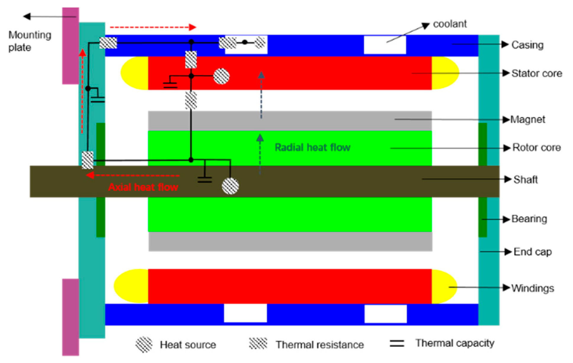
• The heat exchange between the coolant and the motor is much greater than the heat exchange between the casing and the environment. The coolant is the main way to exchange heat with the outside world in PMSMs, so the influence of the outside temperature is ignored. At the same time, the coolant is an important heat source outside the motor, which is collected by the motor controller under real vehicle conditions.
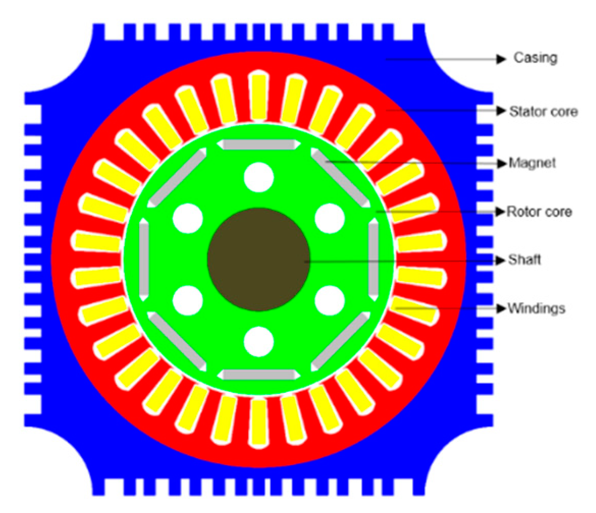
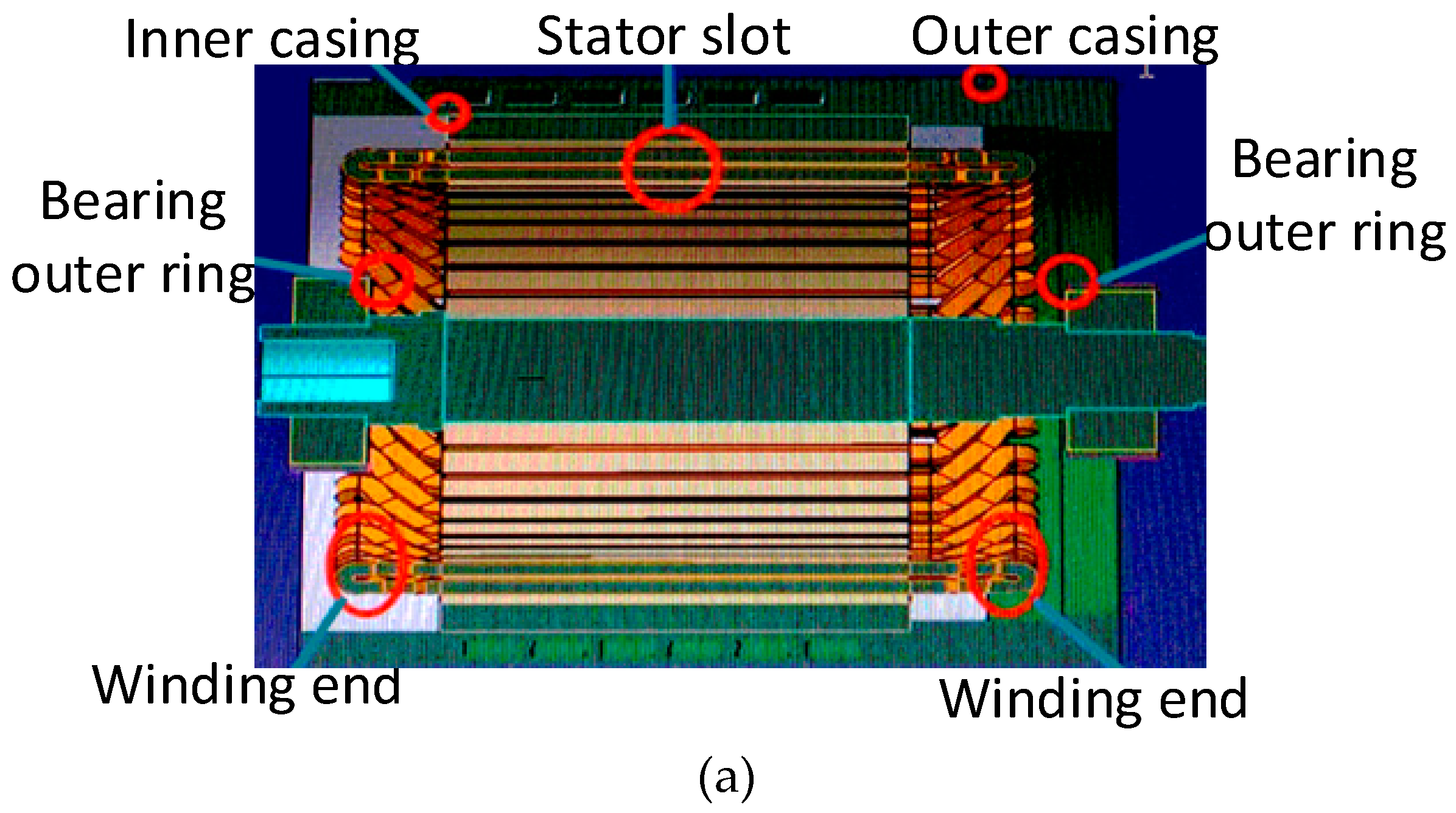
• The motor stator node consists of the stator core and stator windings. These parts are closely connected and have a complicated geometry. If it is treated as a node, the complexity of the model can be greatly simplified. Besides, the stator loss is also an important heat source inside the motor.
• The motor rotor node comprises the rotor core, permanent magnet, and motor shaft. This part is separated from the stator node with the air gap. The rotor iron loss is also an important internal heat source.
• The end cap and the casing are considered as two important nodes in connecting the axial and radial heat paths, making the thermal flow in a complete circuit.
• In water-cooled PMSMs, there is no rib on the motor rotor to increase the convection heat dissipation effect, and the heat transfer effect of the end air is greatly weakened. Thus, the axial heat transfer path through the end air to the end cap is neglected and the topology of the model is thus simplified. The heat path in the axial direction has been considered only in the shaft.

Therefore, this proposed model is optimized according to the structural characteristics of PMSMs for vehicles. As shown in Figure 3, both radial and axial heat transfer paths inside the motor are taken into consideration, and minimum thermal nodes are allowed to model the real thermal flow. The axial heat path mainly considers the thermal flow from the rotor node to the end cap node, which is conducted through the motor shaft. The radial heat path consists of the rotor node, stator node, casing node, and coolant node. The heat source, thermal resistance, and thermal capacity are marked in Figure 3 to indicate how the thermal model is developed according to the motor structure.

According to the radial and axial heat flow of modelled motor, a five-node LPTN is proposed, which is shown in Figure 4. $T_W$, $T_S$, $T_R$, $T_E$, and $T_F$ represent the temperature of the coolant, motor stator, motor rotor, end cap, and motor casing, respectively; $R_{WF}$, $R_{FS}$, $R_{SR}$, $R_{ER}$, and $R_{EF}$ are the thermal resistance between the coolant and the motor casing, the thermal resistance between the motor casing and the motor stator, the thermal resistance between the motor stator and the motor rotor, the thermal resistance between the motor rotor and the endcap, and the thermal resistance between the endcap and the motor casing, respectively; $C_S$, $C_R$, and $C_E$ represent the motor stator heat capacity, motor rotor heat capacity, and motor end cap heat capacity, respectively; $P_S$ and $P_R$ are the loss of the stator and the rotor of the motor, respectively.

2.2. Mathematical Model of Proposed Thermal Model

Similar to Pseudo–Kirchhoff current law, the main equations can be obtained as follows:

$$\{\begin{array}{c}\frac{T_E-T_F}{R_E{}_F}-\frac{T_F-T_S}{R_F{}_S}-\frac{T_F-T_W}{R_W{}_F}=0\\ \frac{C_S \mathrm{d}{T}_S}{\mathrm{d}t}=P_S+\frac{T_F-T_S}{R_F{}_S}+\frac{T_R-T_S}{R_S{}_R}\\ \frac{C_R \mathrm{d}{T}_R}{\mathrm{d}t}=P_R+\frac{T_E-T_R}{R_E{}_R}-\frac{T_R-T_S}{R_S{}_R}\\ \frac{C_E \mathrm{d}{T}_E}{\mathrm{d}t}=-\frac{T_E-T_F}{R_E{}_F}-\frac{T_E-T_R}{R_E{}_R}\end{array}.$$

(1)

The equations contain a linear equation and it can be solved as follows:

$$T_F=\frac{R_E{}_F{R}_F{}_S{T}_W+R_F{}_S{R}_W{}_F{T}_E+R_E{}_F{R}_W{}_F{T}_S}{R_E{}_F{R}_F{}_S+R_E{}_F{R}_W{}_F+R_F{}_S{R}_W{}_F}.$$

(2)

Substituting Equation (2) into the differential Equation (1), the third-order state equation for the simplified thermal model can be described as:

$$\left[\begin{array}{c}\frac{\mathrm{d}{T}_S}{\mathrm{d}t}\\ \frac{\mathrm{d}{T}_R}{\mathrm{d}t}\\ \frac{\mathrm{d}{T}_E}{\mathrm{d}t}\end{array}\right]=\left[\begin{array}{ccc}{a}_{11}& a_{12}& a_{13}\\ a_{21}& a_{22}& a_{23}\\ a_{31}& a_{32}& a_{33}\end{array}\right]\left[\begin{array}{c}{T}_s\\ T_R\\ T_E\end{array}\right]+\left[\begin{array}{ccc}{b}_{11}& b_{12}& 0\\ 0& 0& b_{23}\\ b_{31}& 0& 0\end{array}\right]\left[\begin{array}{c}{T}_w\\ P_s\\ P_R\end{array}\right],$$

(3)

where:

$a_{11}=\frac{-R_E{}_F{R}_F{}_S-R_E{}_F{R}_S{}_R-R_E{}_F{R}_{WF}-R_F{}_S{R}_{WF}-R_S{}_R{R}_{WF}}{C_S{R}_S{}_R\left(R_E{}_F{R}_F{}_S+R_E{}_F{R}_{WF}+R_F{}_S{R}_{WF}\right)}$	$a_{12}=\frac{1}{C_s{R}_{SR}}$
$a_{13}=\frac{R_{WF}}{C_S\left(R_E{}_F{R}_F{}_S+R_E{}_F{R}_{WF}+R_F{}_S{R}_{WF}\right)}$	$b_{11}=\frac{R_E{}_F}{C_S\left(R_E{}_F{R}_F{}_S+R_E{}_F{R}_{WF}+R_F{}_S{R}_{WF}\right)}$
$b_{12}=\frac{1}{C_s}$	$a_{21}=\frac{1}{C_R{R}_{SR}}$
$a_{22}=\frac{-R_E{}_R-R_S{}_R}{C_R{R}_E{}_R{R}_S{}_R}$	$a_{23}=\frac{1}{C_R{R}_{ER}}$
$a_{31}=\frac{R_{WF}}{C_E\left(R_E{}_F{R}_F{}_S+R_E{}_F{R}_{WF}+R_F{}_S{R}_{WF}\right)}$	$a_{32}=\frac{1}{C_E{R}_E{}_R}$
$a_{33}=-\frac{\left(R_E{}_F{R}_F{}_S+R_E{}_R{R}_F{}_S+R_E{}_F{R}_{WF}+R_E{}_R{R}_{WF}+R_F{}_S{R}_{WF}\right)}{C_E{R}_E{}_R\left(R_E{}_F{R}_F{}_S+R_E{}_F{R}_{WF}+R_F{}_S{R}_{WF}\right)}$	$b_{31}=\frac{R_F{}_S}{C_E\left(R_E{}_F{R}_F{}_S+R_E{}_F{R}_{WF}+R_F{}_S{R}_{WF}\right)}$.

It can be concluded from Equation (3) that the stator temperature, rotor temperature, and end cap temperature are the state variables of the system, while the cooling water temperature, stator loss, and rotor loss are system inputs. In order to predict the motor stator temperature, rotor temperature, and end cap temperature, the parameters in the state equation should be identified.

3. Loss Calculation

In the proposed five-node thermal model, the copper loss of the motor winding and the iron loss distributed in the motor rotor and stator are the main heat sources inside the motor. As inputs to the state equation of the motor thermal model, the motor loss needs to be calculated online.

3.1. Permanent Magnet Synchronous Motor Copper Loss Calculation Method

The stator copper loss depends on the stator current and the stator resistance. The stator resistance changes with the temperature, which can be expressed as:

$$R_{\mathrm{s}}=R_{s,20}(1+{\alpha }_{20}(T_s-20 °\mathrm{C})),$$

(4)

where $R_{S,20}$ and ${\alpha }_{20}$ are the stator resistance and the resistance temperature coefficient of the stator winding at the temperature of $20 °\mathrm{C}$, respectively; $T_S$ represents the stator temperature.

The instantaneous stator copper loss can be expressed as:

$$P_{cu}=R_s\times (i_a^2+i_b^2+i_c^2),$$

(5)

where $i_a$, $i_b$, $i_c$ represent the stator three-phase current, respectively.

3.2. Iron Loss Online Calculation

Figure 5a shows the equivalent circuit model with the equivalent iron loss resistance of PMSMs in the d-axis and q-axis. Compared with the general equivalent circuit model, this circuit model is connected with the iron loss equivalent resistance in parallel.

The iron loss can be expressed as:

$$P_F{}_e=\frac{3R_c\left(i_{cd}^2+i_{cq}^2\right)}{2}=\frac{3{\omega }_e{}^2{\left({\psi }_f+L_d{i}_{md}\right)}^2}{2R_c}+\frac{3{\omega }_e{}^2{L}_q{}^2{i}_{mq}{}^2}{2R_c},$$

(6)

where $R_c$ represents the iron loss equivalent resistance; $i_{cd}$ and $i_{cq}$ are the iron loss current in the d-axis and q-axis, respectively; $i_{md}$ and $i_{mq}$ represent the magnetization current in the d-axis and q-axis, respectively.

However, in the conventional equivalent resistance model, the thermal resistance of the stator and the rotor is not distinguished. In the estimation of the motor temperature, the rotor iron loss and the stator iron loss belong to different nodes. Therefore, the equivalent iron loss resistance is regarded as the parallel connection of the stator iron loss equivalent resistance and the rotor iron loss equivalent resistance, respectively:

$$\frac{1}{R_c}=\frac{1}{R_{cr}}+\frac{1}{R_{cs}},$$

(7)

where $R_{cr}$ and $R_{cs}$ are the stator iron loss equivalent resistance and the rotor iron loss equivalent resistance, respectively.

The models of the equivalent iron loss separation for the stator and rotor are shown in Figure 5b.

The stator iron loss power, $P_{Fes}$, and rotor iron loss power, $P_{Fer}$, of the motor can be expressed as:

$$P_{Fes}=\frac{3{\omega }_e{}^2{\left({\psi }_f+L_d{i}_{md}\right)}^2}{2R_{cs}}+\frac{3{\omega }_e{}^2{L}_q{}^2{i}_{mq}{}^2}{2R_{cs}},$$

(8)

$$P_{Fer}=\frac{3{\omega }_e{}^2{\left({\psi }_f+L_d{i}_{md}\right)}^2}{2R_{cr}}+\frac{3{\omega }_e{}^2{L}_q{}^2{i}_{mq}{}^2}{2R_{cr}}.$$

(9)

Under no-load conditions, the iron loss current and the magnetization current become 0. According to Equations (8) and (9), the relationship between the equivalent iron loss resistance and the speed can be expressed as:

$$\begin{array}{l}{R}_{cs}=\frac{3{\omega }_e{}^2{\psi }_f{}^2}{2P_{Fes}}\\ R_{cr}=\frac{3{\omega }_e{}^2{\psi }_f{}^2}{2P_{Fer}}\end{array}$$

(10)

With the help of the finite element simulation method, the iron loss of the motor at different speeds can be simulated and calculated. According to the calculation result and Equation (10), the iron loss resistance of the motor can be estimated. After obtaining the equivalent iron loss resistance, the stator iron loss power and rotor iron loss power can be calculated online according to Equations (8) and (9).

4. Parameter Identification

In order to accurately estimate the motor temperature, it is necessary to identify the parameters in the proposed thermal model. Although the motor model was simplified to reduce the number of parameters, the calculation of these parameters is still very complicated. These parameters can be roughly estimated based on heat transfer theory, but the main disadvantage of this method is the high dependence on the motor geometry model and the impossibility of the real-time execution. Therefore, an offline parameter identification algorithm based on the multiple linear regression model is proposed in this paper under the consideration of the good linear relationship of the state equation for the simplified thermal model. This method does not depend on any motor geometry parameters and material characteristics. Thus, the proposed parameter identification scheme is performed with better robustness, which improves the accuracy of temperature estimation.

After discretizing the state equation of the proposed thermal model, it can be discovered that the time derivative of the state variable (the node temperature) is a linear function related to the state variable and the input (the heat generation), which makes the multiple linear regression algorithm possible to perform offline parameter identification.

The general form of the regression model is:

$$\begin{array}{l}Y=\beta X\\ y_i={\beta }_1{x}_1+{\beta }_2{x}_2+\dots +{\beta }_N{x}_N+{\epsilon }_i(i=1,2,3,\dots ,M)\end{array},$$

(11)

where the dependent variable, $Y$, is a vector consisting of $y_i$; the independent variable, $X$, is a vector consisting of $x_i$. $y_i$ can be approximately expressed as a linear function of the independent variable, $x_1,x_2,x_3,\dots ,x_N$. ${\beta }_1,{\beta }_2,\dots ,{\beta }_N$ represent the regression coefficient, and ${\epsilon }_i$ is the random error.

In order to identify the parameters in the state equation, it is necessary to sample the stator temperature, rotor temperature, end cap temperature, and cooling water temperature of the motor according to Equation (3). The acquired stator temperature, rotor temperature, end cap temperature, and cooling water temperature and the calculated loss are taken as independent variables of the multiple linear regression function, as shown in Equation (12). $T_{si}$, $T_{Ri}$, $T_{Ei}$, $T_{Wi}$, $P_{Si}$, and $P_{Ri}$ $(i=1,2,3\dots M)$ represent the sampled stator temperature, rotor temperature, end cap temperature, and cooling water temperature and the calculated loss, respectively. The derivative of the sampled node temperature is regarded as the dependent variable of the multiple linear regression function, as shown in Equation (13). $Y_1$, $Y_2$, and $Y_3$ are the stator temperature, rotor temperature, and endcap temperature, respectively:

$$X_{sam}=\left[\begin{array}{ccccc}{T}_{S1}& T_{S2}& T_{S3}& \dots & T_{SM}\\ T_{R1}& T_{R2}& T_{R3}& \dots & T_{RM}\\ T_{E1}& T_{E2}& T_{E3}& \dots & T_{EM}\\ T_{W1}& T_{W2}& T_{W3}& \dots & T_{WM}\\ P_{S1}& P_{S2}& P_{S3}& \dots & P_{SM}\\ P_{R1}& P_{R2}& P_{R3}& \dots & P_{RM}\end{array}\right]=\left[\begin{array}{ccccc}{X}_1& X_2& X_3& \dots & X_M\end{array}\right],$$

(12)

$$Y_{sam}=\left[\begin{array}{c}{Y}_1\\ Y_2\\ Y_3\end{array}\right]=\left[\begin{array}{ccccc}\frac{\mathsf{\Delta }{T}_{S1}}{\mathsf{\Delta }t}& \frac{\mathsf{\Delta }{T}_{S2}}{\mathsf{\Delta }t}& \frac{\mathsf{\Delta }{T}_{S3}}{\mathsf{\Delta }t}& \dots & \frac{\mathsf{\Delta }{T}_{SM}}{\mathsf{\Delta }t}\\ \frac{\mathsf{\Delta }{T}_{R1}}{\mathsf{\Delta }t}& \frac{\mathsf{\Delta }{T}_{R2}}{\mathsf{\Delta }t}& \frac{\mathsf{\Delta }{T}_{R3}}{\mathsf{\Delta }t}& \dots & \frac{\mathsf{\Delta }{T}_{RM}}{\mathsf{\Delta }t}\\ \frac{\mathsf{\Delta }{T}_{E1}}{\mathsf{\Delta }t}& \frac{\mathsf{\Delta }{T}_{E2}}{\mathsf{\Delta }t}& \frac{\mathsf{\Delta }{T}_{E3}}{\mathsf{\Delta }t}& \dots & \frac{\mathsf{\Delta }{T}_{EM}}{\mathsf{\Delta }t}\end{array}\right].$$

(13)

According to Equations (3) and (11), the relationship between the regression coefficient, $\beta$, and the parameters of the motor state equation can be expressed as:

$$\beta =\left[\begin{array}{c}{\beta }_1\\ {\beta }_2\\ {\beta }_3\end{array}\right]=\left[\begin{array}{cccccc}{a}_{11}& a_{12}& a_{13}& b_{11}& b_{12}& 0\\ a_{21}& a_{22}& a_{23}& 0& 0& b_{23}\\ a_{31}& a_{32}& a_{33}& b_{31}& 0& 0\end{array}\right].$$

(14)

The regression coefficient can be unbiased estimated using the normal equation according to Equation (15):

$${\beta }_j=Y_j{X}_{sam}{}^T{(X_{sam}{X}_{sam}{}^T)}^{-1}(j=1,2,3).$$

(15)

According to the sampling temperature in each part of the motor and the rate of the temperature change, the parameters of the state equation can be estimated offline.

5. Temperature Online Estimation

After the offline parameter identification, the temperature of the motor can be estimated online. When the parameters in the state equation and losses of the thermal model can be determined, motor temperatures can be estimated online. Two different temperature estimation algorithms are proposed in this paper.

5.1. Temperature Estimation Algorithm Based on State Equation

After discretizing the state equation of the proposed thermal model, the state equation can be expressed as:

$$\left[\begin{array}{c}\frac{\mathsf{\Delta }{T}_S}{\mathsf{\Delta }t}\\ \frac{\mathsf{\Delta }{T}_R}{\mathsf{\Delta }t}\\ \frac{\mathsf{\Delta }{T}_E}{\mathsf{\Delta }t}\end{array}\right]=\left[\begin{array}{ccc}{a}_{11}& a_{12}& a_{13}\\ a_{21}& a_{22}& a_{23}\\ a_{31}& a_{32}& a_{33}\end{array}\right]\left[\begin{array}{c}{T}_s\\ T_R\\ T_E\end{array}\right]+\left[\begin{array}{ccc}{b}_{11}& b_{12}& 0\\ 0& 0& b_{23}\\ b_{31}& 0& 0\end{array}\right]\left[\begin{array}{c}{T}_w\\ P_s\\ P_R\end{array}\right].$$

(16)

After the parameters of the state equation are determined, the motor stator temperature, motor rotor temperature, and motor end cap temperature can be estimated by sampling the cooling water temperature and calculating the stator loss according to Equation (16).

However, the obvious disadvantage of such a method is that an open-loop structure is adopted, so the temperature estimation error is easy to accumulate over time and the temperature accuracy is difficult to ensure. Therefore, temperature estimation based on the Kalman filter algorithm is proposed in this paper.

5.2. Online Temperature Estimation Based on Kalman Filter Algorithm

According to Equation (3), two matrixes are defined as follows:

$$A=\left[\begin{array}{ccc}{a}_{11}& a_{12}& a_{13}\\ a_{21}& a_{22}& a_{23}\\ a_{31}& a_{32}& a_{33}\end{array}\right],$$

(17)

$$B=\left[\begin{array}{ccc}{b}_{11}& b_{12}& 0\\ 0& 0& b_{23}\\ b_{31}& 0& 0\end{array}\right].$$

(18)

With respect to PMSMs, in order to prevent the winding temperature from being too high, a winding temperature sensor is usually installed. Therefore, the winding temperature can be regarded as the measurement variable in Kalman filter scheme. The corresponding measurement equation can be expressed as:

$$T_s=\left[\begin{array}{ccc}1& 0& 0\end{array}\right]\left[\begin{array}{c}{T}_s\\ T_R\\ T_B\end{array}\right].$$

(19)

Definite:

$$H=\left[\begin{array}{ccc}1& 0& 0\end{array}\right].$$

(20)

The specific application of the Kalman filter algorithm regarding the motor temperature estimation is as follows:

1. Considering the process noise and measurement noise of the system, the discrete state equations and measurement equations of the motor thermal model can be expressed as:

$$\begin{array}{l}x(k)=A\cdot x(k-1)+B\cdot u(k)+w(k)\\ y(k)=H\cdot x(k)+v(k)\end{array},$$

(21)

where $x(k)$ represents the state of the system at time k; $u(k)$ represents the control variable, that is, the input variable of the thermal model; $w(k)$ represents the process noise that conforms to the Gaussian distribution, and its covariance is Q; $y(k)$ represents the observation variable of the system at time k, that is, the stator temperature sampled by the stator temperature sensor; $v(k)$ indicates the measurement noise in accordance with the Gaussian distribution, and its covariance is R; A, B are parameter matrices in the system state equation; and H is the parameter matrices in the observation equation.

2. The filter needs to be initialized before making an estimation. The initial values of the state variable, $x$, and error covariance, P, of the priori estimation during each period are calculated as follows:

$$\begin{array}{l}{\widehat{x}}_0^{+}=E(x_0)\\ P_0^{+}=E[(x_0-{\widehat{x}}_0^{+}){(x_0-{\widehat{x}}_0^{+})}^T]\end{array}.$$

(22)

In this paper, the temperature measured by the stator sensor is taken as the initial temperature of the stator, rotor, and end cap.

3. The estimation process for each cycle is divided into five steps:

(a) Based on the estimation results at the previous moment and the state equation, the priori estimation of system state variables is made:

$$x(k|k-1)=A\cdot x(k-1|k-1)+B\cdot u(k).$$

(23)

(b) The error covariance of the priori results is calculated as follows:

$$P(k|k-1)=A\cdot P(k-1|k-1)\cdot A^T+Q,$$

(24)

where P is the error covariance of the priori estimation in first step and Q represents the covariance of the process noise.

(c) $K(k)$ is the filter gain matrix, which is the optimal estimated coefficient matrix of the priori estimation and measurements. It can be expressed as follows:

$$K(k)=P(k|k-1)\cdot H^T\cdot {(H\cdot P(k|k-1)\cdot H^T+R)}^{-1},$$

(25)

where R represents the covariance of the measurement noise.

(d) The priori estimation is corrected based on the filter gain matrix:

$$x(k|k)=x(k|k-1)+K(k)\cdot (y(k)-H\cdot x(k|k-1)).$$

(26)

(e) The error covariance of the priori estimation is adjusted for the next calculation:

$$P(k|k)=(1-K(k)\cdot H)\cdot P(k|k-1).$$

(27)

The different choice of Q and R will result in variance of the temperature prediction. The increase of the value Q will result in improvements of the dynamic performance and steady error, while the rise of the value R will lead to the opposite results. In this study, the calculation of the value, Q, is based on the error between the estimation results of the state equation and the measured values. The covariance matric of the process noise can be expressed as follows:

$$Q=\left[\begin{array}{ccc}C\mathrm{ov}(W_S,W_S)& C\mathrm{ov}(W_S,W_R)& C\mathrm{ov}(W_S,W_E)\\ C\mathrm{ov}(W_R,W_S)& C\mathrm{ov}(W_R,W_R)& C\mathrm{ov}(W_R,W_E)\\ C\mathrm{ov}(W_E,W_S)& C\mathrm{ov}(W_E,W_R)& C\mathrm{ov}(W_E,W_E)\end{array}\right],$$

(28)

where, $W{=[\mathrm{W}}_S,W_R,W_E{]}^T$ is the three-dimensional random variable matric in accordance with the Gaussian distribution, which represents the process noise of the stator, rotor, and end cap, respectively.

Since these three random variables, $W_S,W_R,W_E$, are independent of each other, the covariance of each other is equal to 0, so the covariance matric of the process noise can be simplified as follows:

$$Q=\left[\begin{array}{ccc}C\mathrm{ov}(W_S,W_S)& 0& 0\\ 0& C\mathrm{ov}(W_R,W_R)& 0\\ 0& 0& C\mathrm{ov}(W_E,W_E)\end{array}\right].$$

(29)

The covariance of the process noise can be indicated as follows:

$$\begin{array}{l}C\mathrm{ov}(W_S,W_S)=E\{{[W_S-E(W_S)]}^2\}=\frac{{\Sigma }_{k=1}^n{(w_S(k)-{\overline{W}}_s)}^2}{n-1}\\ C\mathrm{ov}(W_R,W_R)=E\{{[W_R-E(W_R)]}^2\}=\frac{{\Sigma }_{k=1}^n{(w_R(k)-{\overline{W}}_R)}^2}{n-1}\\ C\mathrm{ov}(W_E,W_E)=E\{{[W_E-E(W_E)]}^2\}=\frac{{\Sigma }_{k=1}^n{(w_E(k)-{\overline{W}}_E)}^2}{n-1}\end{array}$$

(30)

where $w_S(k),w_R(k),w_E(k)$ represent the error between the measured temperature and the estimated temperature from the state equation of the stator, rotor, and end cap at time k, which can be obtained according to the previous experimental data in Section 5.1.

Besides, an estimation of the value, Q, is made according to the analog to digital converter(ADC) sampling error.

In each cycle, according to the state equation and measurement equation of the system, the temperature of each part of the motor can be estimated online by applying the Kalman filter algorithm.

6. Experimental Verification

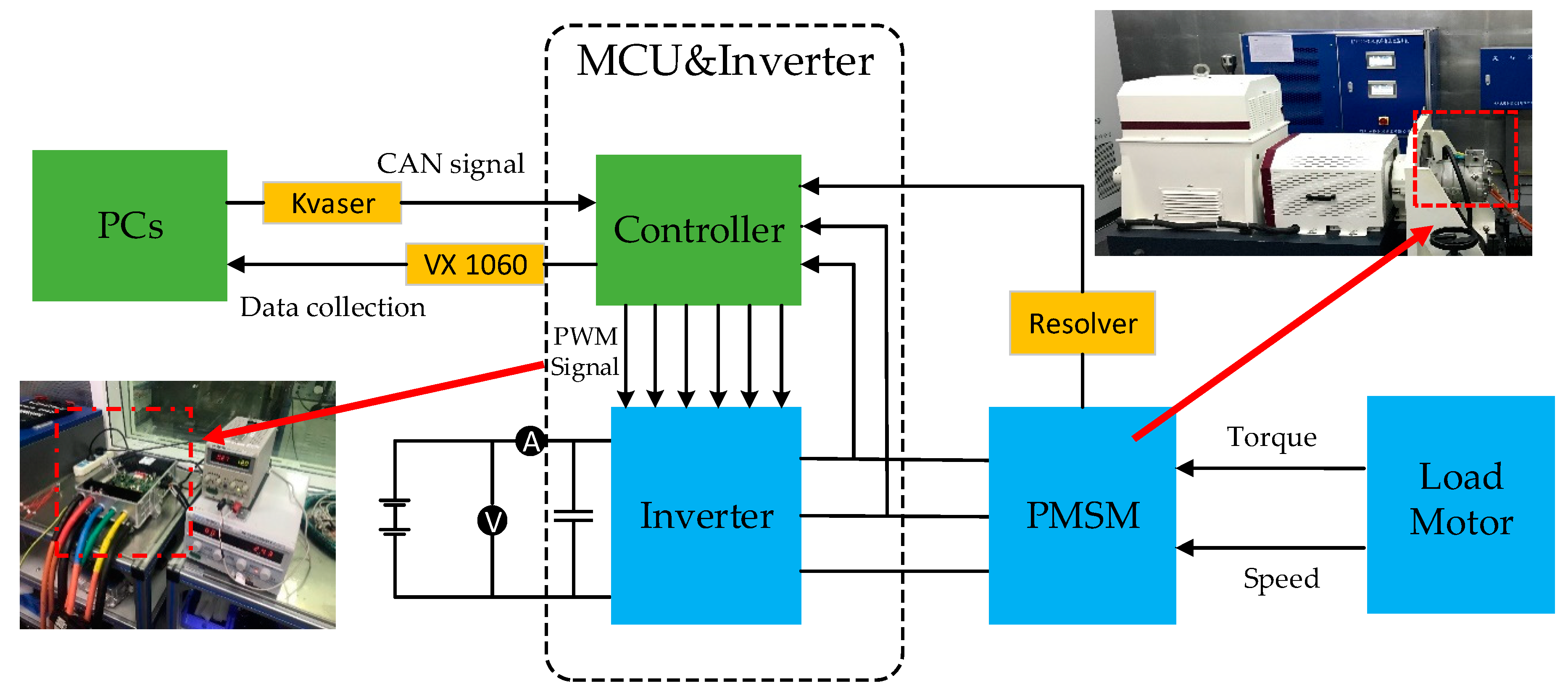
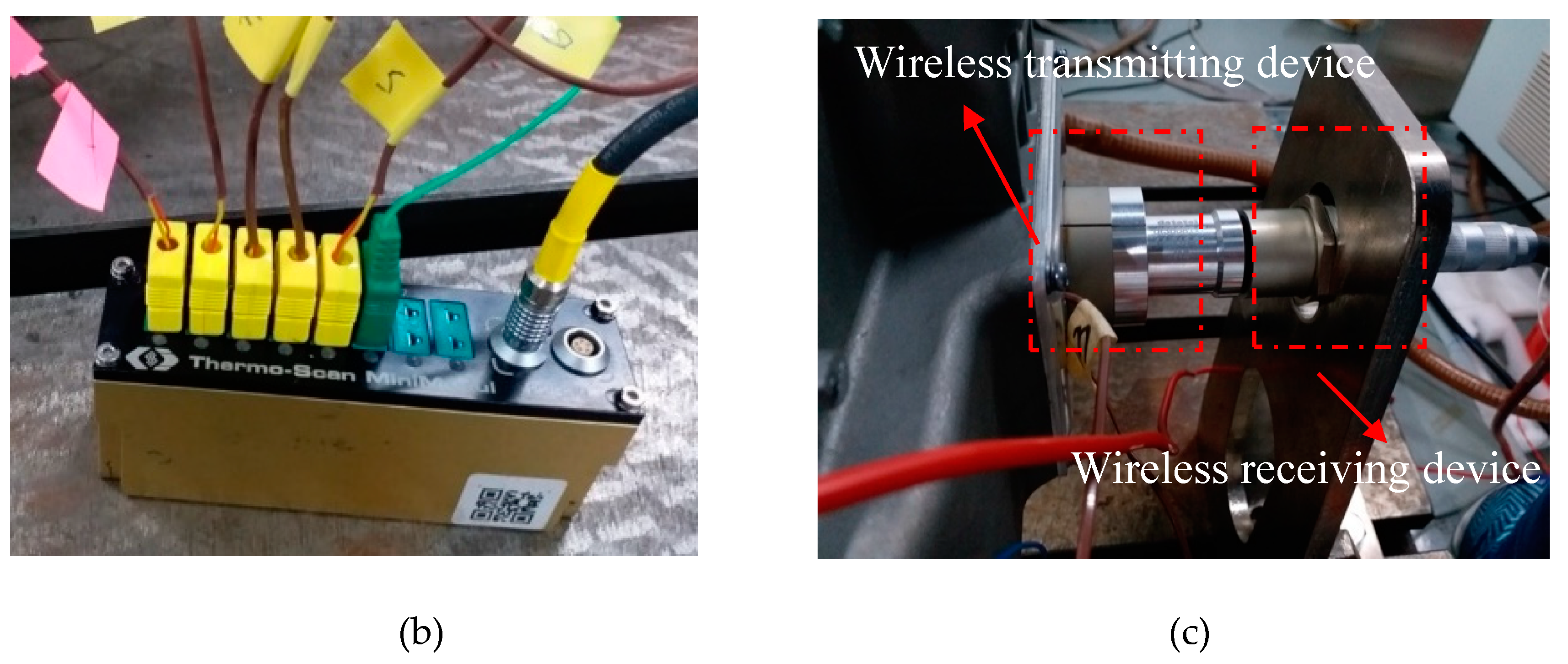
6.1. Experimental Platform

An experiment was conducted to verify the correctness and effectiveness of the proposed model. A four-pole permanent magnet synchronous motor was used for experimental verification. The PMSM parameters used in this experiment are shown in

Table 1. Model parameters of PMSM.

Parameter	Value
rated power	42 Kw
rated torque	100 Nm
rated speed	4000 rpm
inductance in d-axis	0.1425 mH
inductance in q-axis	0.3359 mH
phase resistance	0.016 Ω
poles	4
permanent magnet flux	0.0566 Wb

.

The experimental platform shown in Figure 6 includes PMSM, load motor, motor controller unit (MCU), two PCs, signal conversion device (Kvaser), data collection device (Vector VX1060), speed sensor, and torque sensor. The MCU contains a controller and an inverter. The core of the control border is an Infineon DSP microprocessor (Infineon TC1782). Two PCs were used in this experiment. The first one was used to control the load motor, which provides various load torque for PMSMs. The second one was used to send out a CAN control signal to the MCU, which also collected data through VX1060 and then fed back to the second PC.

The temperatures of the critical positions (the stator, rotor, and end cap) were collected for the purpose of identifying parameters of the state equation. In order to facilitate the temperature acquisition, the motor was modified by embedding K-type temperature sensors. The sensors located in the middle of the stator slot and winding end were applied to measure the stator temperature. In general, since the winding temperature is higher than the temperature in the middle of the stator slot, the winding temperature was regarded as the stator thermal node temperature and the middle temperature of stator slot was used as a reference. The average temperature in the inner casing and the outer casing was obtained to represent the temperature of the casing thermal node, which is neither an input quantity nor a state variable and is the middle variable in the state equation. The acquisition of this temperature node was used to verify the accuracy of the temperature estimation. The temperature in the bearing outer ring was sampled to simulate the end cap node temperature. The distribution of the temperature sensor is shown in Figure 7a. It was sampled by a dedicated temperature acquisition device, as shown in Figure 7b. For the sampling of the rotor temperature, a wireless transmitting and receiving device were used to transmit the internal temperature signal to the external receiving device, as shown in Figure 7c. The coolant temperature was collected by the MCU under real vehicle conditions.

6.2. Parameter Identification at Fixed Speeds

Before the temperature estimation was conducted, the parameters of the state equation were identified. The motor was operated under varying load conditions at 0, 1000, 2000, 3000, 4000, 5000, and 6000 rpm. According to the theoretical analysis in Chapter 4, the parameters of the state equation were identified at each fixed speed based on the multiple linear regression algorithm. By linearly fitting these six sets of parameters, the thermal network model parameters at 7000 rpm were obtained as shown in Equation (31):

$$\beta =\left[\begin{array}{cccccc}-0.0060& 0.0021& -0.0030& 0.0102& 5.5674\times {10}^{-4}& 0\\ -2.5496\times {10}^{-4}& -0.0024& 0.0030& 0& 0& 2.6862\times {10}^{-4}\\ 0.0014& 4.5603\times {10}^{-5}& -0.0058& 0.0051& 0& 0\end{array}\right].$$

(31)

At 7000 rpm, based on the temperature estimation algorithm of the state equation, the stator, rotor and end cap temperatures were estimated by linear fitting using the thermal network model parameters at 7000 rpm. The experimental conditions are shown in

Table 2. Experimental conditions at 7000 rpm.

Duration (min)	Torque (Nm)
5	0
5	20
7	40
30	0

. The result of the fitting parameter estimation was compared with the actual measured result from the sensor, and the comparison is shown in Figure 8.

It can be seen from the experimental results that with the torque changes, the result of the fitting parameter estimation keeps the same trend as the measured result of the sensor, indicating that the thermal model can accurately predict the motor temperature change.

6.3. Temperature Estimation Under Complex Conditions

After the identification of the thermal model parameters, an independent continuous heating and cooling experiment at different speeds was carried out, and the duration of the experiment under the complex condition was about 4 h, as shown in Figure 9. The stator winding temperature, rotor temperature, and end cap temperature were investigated. The temperature directly measured by the temperature sensor, the temperature calculated by the motor state equation, and the temperature estimated based the Kalman filter algorithm were compared, which is shown in Figure 9. In Figure 9, V/Vn and T/Tn represent the ratio of the operating speed and rated speed and the ratio of the output torque and the rated torque, respectively.

From Figure 9, the following conclusions can be made:

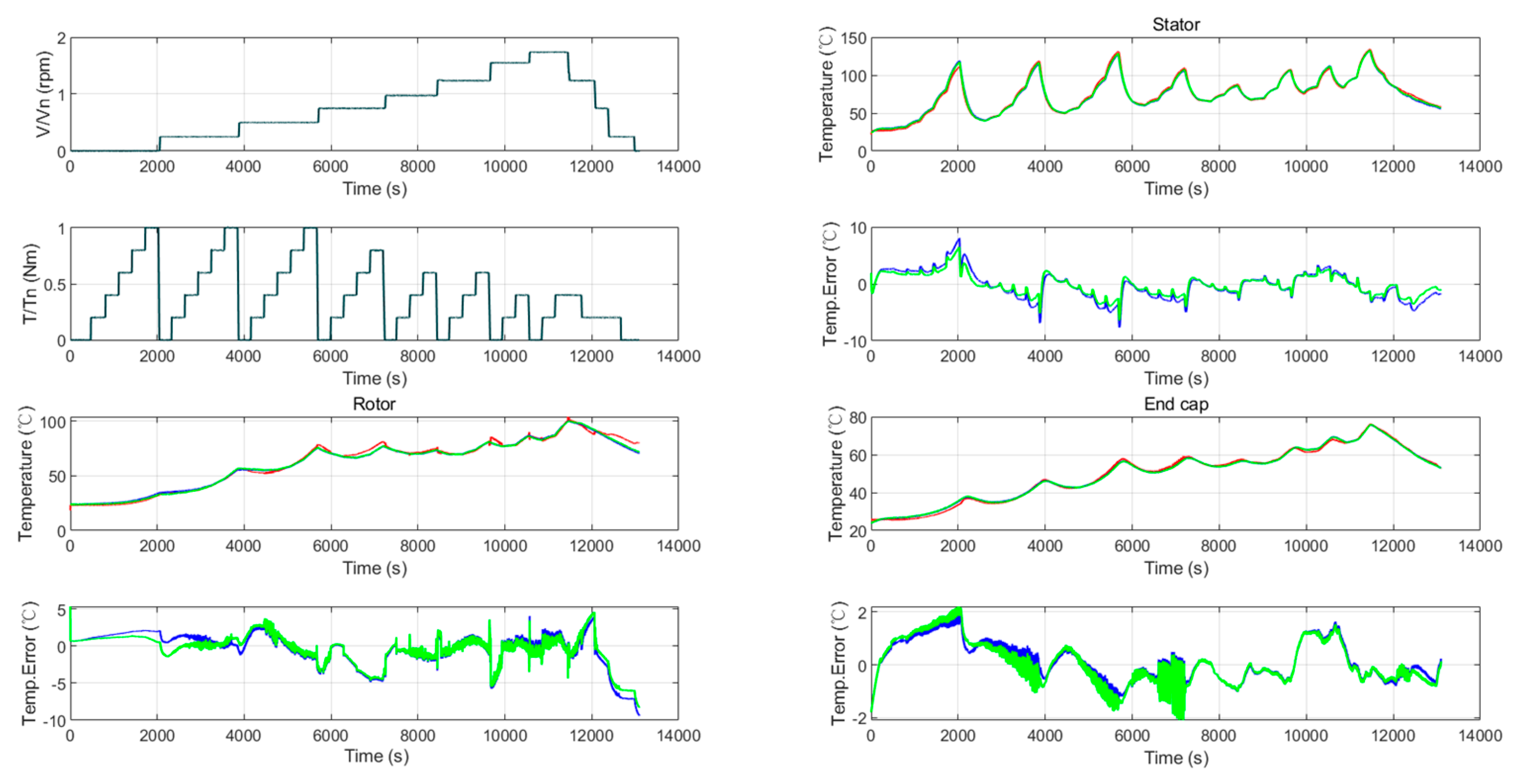
• By comparing the temperature estimation results, it was found that the stator, rotor, and end cap temperatures change with different operation conditions. Figure 9 shows that as the speed increases, the temperature of the rotor and end cap increases. During each period of torque change, the temperature will fluctuate, but the fluctuation range is not large within the range of 10 °C. Regarding the stator temperature variation, the temperature rises when the motor accelerates; but during each period of torque change, the temperature fluctuates greatly. When the range of torque change reduces, temperature fluctuations also decrease. Before 6000 s, the torque fluctuation changes in the range of 0–5 Nm, and the fluctuation range of the stator temperature exceeds 70 °C. After the moment of 6000 s, the temperature fluctuation range is reduced to 30 °C as the torque fluctuation decreases. It shows that the variation of the torque fluctuation range has a greater influence on the estimation of the stator temperature but has less impact on the rotor and end cap temperature estimation. This is because when the torque is large, the current also becomes large. According to Equations (8) and (9), the change of the current and speed will result in variation of the stator and rotor loss. In addition, the change of working conditions will also lead to changes in the thermal resistance and capacity of the thermal model, so the motor temperature change is the result of multiple parameters. Thus, by establishing a lumped parameter network thermal model of the motor, the change in motor temperature can be accurately predicted.
• From Figure 9, it can be seen that at the moment of sudden torque change, the temperature waveform will have a sharp peak, and the thermal model can quickly respond to the change of the working condition. The difference between the estimated temperature and the measured temperature will not exceed 10 °C at the moment of change. Therefore, the equivalent thermal model proposed in this paper has good robustness and observation accuracy.
• For the temperature estimation in PMSMs, the rotor temperature is critical, since the rotor temperature is not easily available to sensors. The results show that the rotor temperature error is within a range of ±5 °C in most cases, which indicates the improved prediction accuracy of the proposed model. Regarding the stator temperature estimation, at the moment, when the load condition changes, the error becomes large, but the proposed model can quickly follow the temperature change, resulting in a reduction of error. The rapid response ability shows that the proposed model has a better robustness. Besides, when the fluctuation of the load reduces, the accuracy will increase. Except for moments when the load condition changes sharply, the steady error of the stator temperature estimation was observed to be around 0 °C. The temperature error is smaller regarding the end cap, with a variation of 2 °C.
• The estimation performance of the state equation estimation and the Kalman filter algorithm was compared. As for the stator and rotor, the temperature error of the Kalman filter method is smaller than that of state equation estimation. The reason lies in the fact that the state equation estimation method adopts an open-loop structure, and the temperature prediction error is easy to accumulate over time. Since the estimation error of the end cap is smaller by only around 2 °C, the performance of these two methods can be thought to be the same.
• In the experiment, the temperature estimation error may result from the following reasons: The temperature measurement device is affected by the interference of the motor itself; the thermal model comes from the simplification of LPTN; and the open-loop estimation error based on the state equation is susceptible to time accumulation.

In summary, the five-node LPTN proposed in this paper is not only suitable for estimating the motor temperature at a fixed speed but also for the temperature of the motor under complex conditions. At the same time, the experimental results also verify the correctness of the model parameter identification algorithm based on the multiple linear regression method, and the accuracy of the temperature estimation algorithm based on the state equation and the Kalman filter.

7. Conclusions

A five-node simplified lumped parameter network model was proposed and the multiple linear regression algorithm was applied to identify parameters of the state equation. The temperature estimation algorithm based on the state equation and Kalman filter algorithm was proposed to predict the motor temperature. It can be concluded that:

• The proposed lumped parameter network model is simple, and the thermal model order is low. Therefore, it is easier and faster to implement online estimation in an embedded system. Besides, both the radial and axial heat transfer paths inside the motor were considered, and minimum thermal nodes were applied to model the complete thermal circuit. In this way, the accuracy of thermal model was improved.
• The multiple linear regression algorithm was utilized to identify the parameters of the state equation. This method does not depend on the structural parameters of the motor. It is not necessary to identify each specific parameter in the thermal model, and only the parameters in the state equation need to be identified.
• The temperature estimation algorithm based on the state equation was used to predict the motor temperature. However, the disadvantage of this method is that error easily accumulates over time based on an open-loop structure. Thus, the Kalman filter algorithm was proposed to estimate the motor temperature online. The experimental results showed that the temperature estimation error does not exceed ±5 °C in most cases, which indicates that the proposed model can accurately predict the stator, rotor, and end cap temperature of the motor. The experimental results also verified the accuracy and effectiveness of the parameter identification algorithm and temperature estimation algorithm.

In the future, other methods for measuring the rotor temperature will be studied due to the high cost of the special rotor temperature acquisition equipment, so that the proposed thermal model has a wide application range.

References

1. Pietrusewicz, K.; Waszczuk, P.; Kubicki, M. MFC/IMC Control Algorithm for Reduction of Load Torque Disturbance in PMSM Servo Drive Systems. Appl. Sci. 2018, 9, 86. [Google Scholar] [CrossRef]
2. Mehrjou, M.R.; Mariun, N.; Misron, N.; Radzi, M.A.M.; Musa, S. Broken Rotor Bar Detection in LS-PMSM Based on Startup Current Analysis Using Wavelet Entropy Features. Appl. Sci. 2017, 7, 845. [Google Scholar] [CrossRef]
3. Liang, H.; Chen, Y.; Liang, S.; Wang, C. Fault Detection of Stator Inter-Turn Short-Circuit in PMSM on Stator Current and Vibration Signal. Appl. Sci. 2018, 8, 1677. [Google Scholar] [CrossRef]
4. Boglietti, A.; Cavagnino, A.; Lazzari, M.; Pastorelli, M. A simplified thermal model for variable-speed self-cooled industrial induction motor. IEEE Trans. Ind. Appl. 2003, 39, 945–952. [Google Scholar] [CrossRef]
5. Boglietti, A.; Cavagnino, A.; Staton, D.; Shanel, M.; Mueller, M.; Mejuto, C. Evolution and Modern Approaches for Thermal Analysis of Electrical Machines. IEEE Trans. Ind. Electron. 2009, 56, 871–882. [Google Scholar] [CrossRef]
6. Boglietti, A.; Popescu, M.; Staton, D.; Cavagnino, A. Thermal Model and Analysis of Wound-Rotor Induction Machine. IEEE Trans. Ind. Appl. 2013, 49, 2078–2085. [Google Scholar] [CrossRef]
7. Zhang, B.; Qu, R.; Wang, J.; Xu, W.; Fan, X.; Chen, Y. Thermal Model of Totally Enclosed Water Cooled Permanent Magnet Synchronous Machines for Electric Vehicle Applications. IEEE Trans. Ind. Appl. 2015, 51, 1. [Google Scholar] [CrossRef]
8. Gao, Z.; Colby, R.S.; Habetler, T.G.; Harley, R.G. A Model Reduction Perspective on Thermal Models for Induction Machine Overload Relays. IEEE Trans. Ind. Electron. 2008, 55, 3525–3534. [Google Scholar] [CrossRef]
9. Dorrell, D.; Dorrell, D. Combined Thermal and Electromagnetic Analysis of Permanent-Magnet and Induction Machines to Aid Calculation. IEEE Trans. Ind. Electron. 2008, 55, 3566–3574. [Google Scholar] [CrossRef]
10. Alberti, L.; Bianchi, N. A Coupled Thermal–Electromagnetic Analysis for a Rapid and Accurate Prediction of IM Performance. IEEE Trans. Ind. Electron. 2008, 55, 3575–3582. [Google Scholar] [CrossRef]
11. Reigosa, D.D.; Garcia, P.; Briz, F.; Raca, D.; Lorenz, R. Modeling and Adaptive Decoupling of High-Frequency Resistance and Temperature Effects in Carrier-Based Sensorless Control of PM Synchronous Machines. IEEE Trans. Ind. Appl. 2010, 46, 139–149. [Google Scholar] [CrossRef]
12. Reigosa, D.D.; Briz, F.; García, P.; Guerrero, J.M.; Degner, M. Magnet temperature estimation in surface PM machines using high frequency signal injection. IEEE Trans. Ind. Appl. 2009, 46, 1468–1475. [Google Scholar] [CrossRef]
13. Reigosa, D.D.; García, P.; Briz, F.; Raca, D.; Lorenz, R.D. Modeling and Adaptive Decoupling of Transient Resistance and Temperature Effects in Carrier-Based Sensorless Control of PM Synchronous Machines. In Proceedings of the 2008 IEEE Industry Applications Society Annual Meeting, Edmonton, AB, Canada, 5–9 October 2008; pp. 1–8. [Google Scholar]
14. Ganchev, M.; Kral, C.; Wolbank, T. Sensorless Rotor Temperature Estimation of Permanent Magnet Synchronous Motor under Load Conditions. In Proceedings of the 38th Annual Conference on IEEE Industrial Electronics Society (IECON 2012), Montreal, QC, Canada, 25–28 October 2012; pp. 1999–2004. [Google Scholar]
15. Qu, R.; Fan, X.; Li, J.; Li, D.; Zhang, B.; Wang, C. Ventilation and Thermal Improvement of Radial Forced Air-Cooled FSCW Permanent Magnet Synchronous Wind Generators. IEEE Trans. Ind. Appl. 2017, 53, 3447–3456. [Google Scholar]
16. Lu, Y.; Liu, L.; Zhang, D. Simulation and Analysis of Thermal Fields of Rotor Multislots for Nonsalient-Pole Motor. IEEE Trans. Ind. Electron. 2015, 62, 7678–7686. [Google Scholar] [CrossRef]
17. Camilleri, R.; Howey, D.A.; McCulloch, M.D. Predicting the Temperature and Flow Distribution in a Direct Oil-Cooled Electrical Machine with Segmented Stator. IEEE Trans. Ind. Electron. 2016, 63, 82–91. [Google Scholar] [CrossRef]
18. Oliver, W.; Böcker, J. Global identification of a low-order lumped-parameter thermal network for permanent magnet synchronous motors. IEEE Trans. Energy Convers. 2015, 31, 354–365. [Google Scholar]
19. Jaljal, N.; Trigeol, J.-F.; Lagonotte, P. Reduced Thermal Model of an Induction Machine for Real-Time Thermal Monitoring. IEEE Trans. Ind. Electron. 2008, 55, 3535–3542. [Google Scholar] [CrossRef]
20. Kral, C.; Haumer, A.; Bin Lee, S. A Practical Thermal Model for the Estimation of Permanent Magnet and Stator Winding Temperatures. IEEE Trans. Power Electron. 2014, 29, 455–464. [Google Scholar] [CrossRef]
21. Huber, T.; Peters, W.; Böcker, J. A Low-Order Thermal Model for Monitoring Critical Temperatures in Permanent Magnet Synchronous Motors. In Proceedings of the 7th IET International Conference on Power Electronics, Machines and Drives (PEMD 2014), Manchester, UK, 8–10 April 2014. [Google Scholar]
22. Nerg, J.; Rilla, M.; Pyrhonen, J. Thermal Analysis of Radial-Flux Electrical Machines with a High Power Density. IEEE Trans. Ind. Electron. 2008, 55, 3543–3554. [Google Scholar] [CrossRef]
23. Daniel, D.; Oliver, W.; Böcker, J. Global Identification Methods for Low-Order Lumped-Parameter Thermal Networks Used in Permanent Magnet Synchronous Motors. In Proceedings of the 2017 IEEE 12th International Conference on Power Electronics and Drive Systems (PEDS), Honolulu, HI, USA, 12–15 December 2017; pp. 126–133. [Google Scholar]
24. Huber, T.; Peters, W.; Böcker, J. Monitoring critical temperatures in permanent magnet synchronous motors using low-order thermal models. In Proceedings of the 2014 International Power Electronics Conference (IPEC-Hiroshima 2014—ECCE ASIA), Hiroshima, Japan, 18–21 May 2014; pp. 1508–1515. [Google Scholar]
25. Boseniuk, F.; Ponick, B. Parameterization of transient thermal models for permanent magnet synchronous machines exclusively based on measurements. In Proceedings of the 2014 International Symposium on Power Electronics, Electrical Drives, Automation and Motion (SPEEDAM 2014), Ischia, Italy, 18–20 June 2014; pp. 295–301. [Google Scholar]
26. Demetriades, G.; De La Parra, H.; Andersson, E.; Olsson, H. A Real-Time Thermal Model of a Permanent-Magnet Synchronous Motor. IEEE Trans. Power Electron. 2010, 25, 463–474. [Google Scholar] [CrossRef]
27. Fan, J.X.; Zhang, C.N.; Wang, Z.F. Thermal Analysis of Permanent Magnet Motor for the Electric Vehicle Application Considering Driving Duty Cycle. IEEE Trans. Magn. 2010, 46, 2493–2496. [Google Scholar] [CrossRef]
28. Chen, Q.X.; Zou, Z.Y.; Cao, B.G. Lumped-Parameter Thermal Network Model and Experimental Research of Interior PMSM for Electric Vehicle. CES Trans. Electr. Mach. Syst. 2017, 3, 367–374. [Google Scholar]
29. Lan, Z.Y.; Wei, X.C.; Chen, L.H. Thermal Analysis of PMSM Based on Lumped Parameter Thermal Network Method. In Proceedings of the 2016 19th International Conference on Electrical Machines and Systems (ICEMS), Chiba, Japan, 13–16 November 2016. [Google Scholar]
30. Mellor, P.H.; Turner, D.R. Real Time Prediction of Temperatures in an Induction Motor Using a Microprocessor. Electr. Mach. Power Syst. 1988, 15, 333–352. [Google Scholar] [CrossRef]
Figure 1. Complete thermal model of the induction motor.
Applsci 09 03158 g001
Figure 2. Cross section of modelled motor.
Applsci 09 03158 g002
Figure 3. Radial and axial heat flow of the modelled motor.
Applsci 09 03158 g003
Figure 4. Proposed thermal network model.
Applsci 09 03158 g004
Figure 5. Dynamic equivalent circuit of PMSM in d-axis and q-axis: (a) considering iron loss; (b) iron loss separation.
Applsci 09 03158 g005
Figure 6. Test bench for the temperature measurement.
Applsci 09 03158 g006
Figure 7. Experimental platform: (a) Temperature sensor distribution; (b) temperature acquisition equipment; (c) wireless transmitting and receiving devices.
Applsci 09 03158 g007aApplsci 09 03158 g007b
Figure 8. Temperature comparison at 7000 rpm.
Applsci 09 03158 g008
Figure 9. Experiment under complex condition: Measured (red); state equation (blue); Kalman filter (green).
Applsci 09 03158 g009