Review

AUV Adaptive Sampling Methods: A Review

1
Australian Maritime College, University of Tasmania, Launceston 7250, TAS, Australia
2
Department of Ocean and Naval Architectural Engineering, Memorial University of Newfoundland, St. John’s, NL A1C 5S7, Canada
3
School of Marine Sciences, Sun Yat-sen University, Zhuhai 519082, Guangdong, China
*
Author to whom correspondence should be addressed.
Appl. Sci. 2019, 9(15), 3145; https://doi.org/10.3390/app9153145
Submission received: 16 July 2019 / Revised: 26 July 2019 / Accepted: 29 July 2019 / Published: 2 August 2019
(This article belongs to the Special Issue Underwater Robots in Ocean and Coastal Applications)

Abstract

:
Autonomous underwater vehicles (AUVs) are unmanned marine robots that have been used for a broad range of oceanographic missions. They are programmed to perform at various levels of autonomy, including autonomous behaviours and intelligent behaviours. Adaptive sampling is one class of intelligent behaviour that allows the vehicle to autonomously make decisions during a mission in response to environment changes and vehicle state changes. Having a closed-loop control architecture, an AUV can perceive the environment, interpret the data and take follow-up measures. Thus, the mission plan can be modified, sampling criteria can be adjusted, and target features can be traced. This paper presents an overview of existing adaptive sampling techniques. Included are adaptive mission uses and underlying methods for perception, interpretation and reaction to underwater phenomena in AUV operations. The potential for future research in adaptive missions is discussed.

1. Introduction

Autonomous underwater vehicles (AUVs) are unmanned marine robots. Owing to their mobility and increased ability to accommodate sensors, they have been used for a broad range of oceanographic missions, such as surveying underwater plumes and other phenomena, collecting bathymetric data and tracking oceanographic dynamic features. As the name suggests, autonomous behaviours [1] are one of their capabilities. Although defining autonomy in robotics can be ambiguous and the minimum level of autonomy depends on context, this paper is only concerned with decision autonomy [2] of unmanned robots. Seto [1] discriminated between autonomous behaviour and intelligent behaviour. The former is a collection of actions for known situations in which the robot is not allowed to adapt its tasks in situ. The latter, on the other hand, is the capability that the robot can adapt and complete its mission by reacting to unforeseen events. Intelligent behaviours of an AUV require a high level of autonomy. They include the ability to make decisions, interpret in-situ sensor data, diagnose the problems, make inference from data, suggest solutions and adapt the planned mission.
Demand for a high level of autonomy is increasing as the application of underwater robotics has expanded. Depending on the dynamics of a feature, different strategies and sampling methods may apply. Some ocean features evolve highly dynamically over time, some others relatively less so. If the spatial and temporal scales are known, the primary perspective of sampling will be how to adjust sampling distribution for measurements in accordance with the local variance. Scales also determine the number of survey agents that need to be involved. The mesoscale oceanographic features (in the order of 10 km) may require the coordinated effort of a fleet of platforms rather than a single vehicle, in order to obtain a more synoptic and cohesive data set [3].
This paper reviews the state-of-the-art adaptive sampling methods that have been used in the last few decades in AUV operations. The review aims to put into context the various methods that have been proposed outlining their advantages and disadvantages for future researchers in the field. Section 2 elucidates the process of adaptive sampling. Section 3, Section 4 and Section 5 describe various adaptive sampling techniques. They are described in accordance with subcategories: Targets, mission objectives and multi-vehicle networking, as listed in Table 1. Section 6 concludes this study.

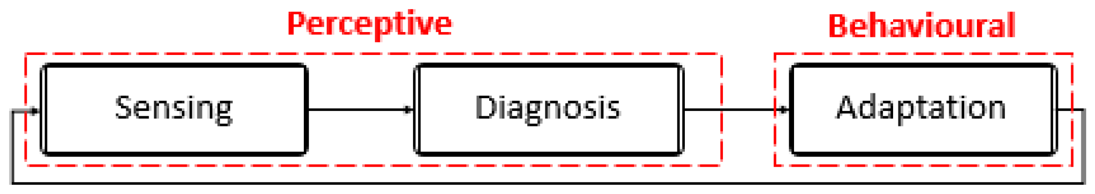
2. Process of Adaptive Sampling

An AUV is normally fitted with sensors in order to undertake a mission. After sensor measurements are collected, they are analysed and interpreted into meaningful data. In an adaptive mission and based on the analysed data, an existing mission plan may be modified or renewed to optimise the AUV path for subsequent measurements.
One example of an adaptive sampling procedure may include: (1) investigate an initial set of sparse observations, which leads to the question of where to take the next measurements, and (2) revisit and conduct a finer scale survey. The underlying autonomous structure of the procedure requires three basic segments: sensing, diagnosis and adaptation. They resemble the cognition process of many biophysical entities. These steps are recursively executed in a closed loop process as shown in Figure 1. In the perceptive phase, the collected measurements are interpreted into meaningful data, while conforming to the current mission plan. Then, in the behavioural phase, details of the mission plan are updated to suit the mission goal/s. A description of each step is given below.
Sensing: An AUV can acquire knowledge about its surroundings through taking measurements using a variety of sensors. Sensing the environment or perceiving the phenomena is the first step, yet it is the most crucial part in the course of operation of the AUV. It allows the AUV to comprehend the survey area, and therefore, to plan a better path. Especially in an unstructured environment, the AUV must rely on its sensor measurements to gather information. This sensing step has significance in two regards: being closely related to the vehicle survey path and appropriate sensor selection.
The path or trajectory of unmanned vehicles influences the result of sensing performance. For example, algal blooms in the ocean appear in the horizontal plane at various depths over time. Therefore, a vertical saw-tooth AUV trajectory is commonly adopted to delineate their vertical migration. In short, the trajectory of the vehicle is determined depending on the distribution of the target in water.
Some measurements are simple parameters that are readily extracted and easily interpreted, such as the temperature of the ambient water or the speed of the AUV. The depth of the AUV is measured by using a pressure sensor. More complicated sensors, such as fluorometers or an underwater mass spectrometer, take biological or chemical measurements that require further interpretation to convert them into meaningful data. Selection of appropriate sensors is the key in successful sensing or detection. Table 2 summarises a list of example sensors for several different features.
Diagnosis: After the measurements are taken in the previous step, they undergo diagnosis. The ultimate objective of this step is to make the best decisions to autonomously serve the end goal via processing sampled information. Diagnosis is crucial, but challenging, as it requires the ability to analyse and interpret the collected measurements through associated data. This is especially true when the measurements are not straightforward and require further processing to turn them into useful information.
The collected in-situ measurements should usually undergo several processes prior to making any decisions by the AUV. Firstly, the obtained measurements are processed using a certain type of filter as all sensor measurements in robotics are raw, imperfect and subject to errors. A substantial amount of sensor noise makes the measurements less reliable. Such ambiguities and uncertainties (in vehicle motions and sensor measurements) are an inherent issue in robotic missions. Therefore, a probabilistic approach is usually taken as a solution, as opposed to a deterministic approach (e.g., [1]). Secondly, onboard analysis capability in modern AUV technology enables sensor readings to be converted into meaningful data values that can be used in decision autonomy. How adeptly an AUV can perceive its own state and its environment relies on data analysis and the analytical algorithm design. They can vary from a binary structure, which simply defines the presence or absence of a phenomena of interest, to a wider range of state estimates, which leads to a consequent action to be taken in the next step.
Appropriate thresholds are often requisites for successful diagnosis. They represent the adequate level at which scientists believe the measure is worth sampling. Threshold values can be unit or unit-less scalar attributes such as temperature (°C), concentration (mg/L, ppb), number of particles, salinity (ppt) and water velocity (m/s). They could also be instantly calculated values such as gradients. The values are given from the beginning of a mission if the survey area is sufficiently known or if the mission goal is to seek the location of the target thresholds in particular. Variable thresholds, on the other hand, consistently change and provide a high level of flexibility in terms of survey range, especially in the early stage of the event, where there is limited basic information available [4].
Adaptation: The last segment, adaptation takes charge of executing adaptive commands and the calculated value is delivered to the actuation system. The adaptation commands include redesigning the mission plan, modifying the survey pattern and updating the vehicle trajectory. Successful adaptation enables overall sampling performance of the AUV to be truly autonomous.
The Adaptation step falls under the realm of control. It allows adapting the specifications of the original mission so that a user-specified mission goal is achievable. Three approaches to control architectures are introduced by Hagen et al. [2] as shown in Table 3.
The actual experimental records and data from adaptive sampling approaches in oceanographic surveys have been limited, although the notion of it has long been addressed. A variety of existing adaptive sampling missions using AUV(s) are discussed in the following Section 3, Section 4 and Section 5.

3. Target of Interest

Targeted marine phenomena or features can be categorised into physical, biological or chemical parameters depending on the measurable proxies and their inherent characteristics, respectively. Each target may take and evolve into a different form featuring different physical, biological and chemical properties in water. In accordance with their properties and dynamics, the sampling strategy may vary. This section provides a variety of adaptive sampling approaches that have been applied in the past for each of these targets.

3.1. Physical Features

Three typical physical features in oceanographic research are introduced here: thermoclines, upwelling and internal waves. A thermocline is a thermally stratified body of water in which the vertical temperature changes significantly with depth [5]. Upwelling is an ocean process near coastal regions caused by a combination of wind and Ekman transport, which brings a cold deep-water mass upward while displacing the surface water in an offshore direction [6]. Internal waves at an internal interface (usually a density difference) are generated by a deep-sea earthquake or when a tidal wave meets a major obstacle, such as an ocean ridges or underwater mountains. As internal waves transport heat and nutrient-rich water upward into the surface layer, they are frequently observed in regions where a strong thermocline is present by Petillo [7]. An upwelling front can be sensed by encountering a region of vertical homogeneity of temperature, salinity and density in an otherwise stratified water column. Thus, temperature is a good indicator to sense the above physical phenomena in the ocean.

3.1.1. Thermoclines

A vertical gradient method [8,9] was proposed to use an AUV to identify a thermocline and gave a demonstration in a dam reservoir in the Douro River, Northern Portugal. They applied a depth adaptation algorithm implemented on a small-size MARES AUV, so that the vehicle could stay in the vicinity of the thermocline. They simplified the thermocline profile by dividing it into three layers: a layer they named thermocline (a thin layer in the water column having the greatest linear gradient), a deep-water layer (the least dynamic and the coldest zone lying below the thermocline layer in which the temperature decreased slowly with depth increase) and a mixed layer (a relatively dynamic zone above the thermocline layer due to various influencing factors from the atmosphere). This layered ocean model of the temperature structure was originally proposed by Clabon [10]. Utilising a state machine, the algorithm achieved detection and tracking of a thermocline by comparing the vertical temperature gradient in each depth bin with a set of thresholds in real time.
Petillo et al. proposed [11] an average gradient method. Their method started with an initial deep dive to acquire a complete temperature profile from the surface to the operational depth limit of the AUV. The result from this initial yo-yo determined the size of the depth bins, also referred to as the vertical depth levels. The depth bin size in their algorithm is highly dependent on the water depth and the thermocline range. The guideline of the scale analysis used is shown in Table 4. The next step was to average the data over the depth bins and then calculate the rates of temperature change over the depth change (vertical derivatives). Any vertical derivatives greater than the average value were assessed to be within the thermocline.
Zhang et al. [12] focused on the maximum value of vertical temperature gradient to detect a thermocline and its corresponding depth to guide an AUV to successively track the thermocline. In each ascent and descent leg, the peak gradient was saved and used to establish the subsequent target diving depth. They also allowed an additional extension depth, so as to be able to capture the genuine peak spots. Having this extension depth helped to deal with the large vertical depth variation that is often found in an undulated thermocline and helps prevent the AUV from getting trapped in a local maximum. They successfully applied their maximum gradient method on a Tethys AUV mission in Monterey Bay.
Woithe and Kremer [13] presented a dichotomous triggering method, in benchtop simulations and during a short deployment of a glider in the Atlantic Ocean. This method is straightforward in the sense that depth bins are only specified by two variables, temperature and depth (a priori). There are no initial deep dives, headings or waypoints requirements. The transition between behaviours was triggered by events of interest with a fixed threshold parameter of 3 °C/4 m. The average temperature of depth bins at each point was evaluated by dichotomous criteria, as to whether it was above or below the threshold. This event-driven performance may include changing a glider’s target depth or returning to a previous state or even a more complicated transition mechanism, if desired.
Later, Woithe and Kremer [5] introduced a feature-based gradient method, a new hybrid adaptive sampling algorithm combining the average gradient method [11] and the maximum gradient method [12]. The two gradient methods were combined to complement each other. Based on the initially targeted thermocline (sensed by CTD), they aimed to investigate the chlorophyll concentration level (assessed by ECO-Puck and FIRe sensors). The average gradient algorithm was triggered to activate the ECO-Puck sensor when thermocline was detected by CTD readings. The maximum gradient algorithm takes control by triggering the puck sensor if the peaks kept being detected during three consecutive ascending–descending legs. Then, when a sufficient concentration of chlorophyll is sensed by ECO-Puck, the second sensor (FIRe) was triggered.
While the method of [11] was governed by the averaged-temperature gradient, both [9] and [12] used the maximum gradients. The vertical gradient method [9] might be more beneficial in the case of relatively thicker thermoclines, as they have a weaker vertical gradient than thinner thermoclines because smaller bins led to large errors in their gradient estimation. Meanwhile, the approach of Zhang et al. [12] is somewhat simpler, as it reduces the necessity of the output from three sensors to generate thresholds, and it was found to work robustly for thinner thermoclines with large vertical undulations by making use of temperature range in each yo-yo profile. A distinct comparison was made between the traditional yo-yo survey pattern and the narrow yo-yo of the adaptive sampling method by Cruz [14], proving that survey distance is effectively reduced by adopting the flipping attitude (ascending and descending) dynamically so as to closely track the thermocline.

3.1.2. Upwelling Fronts

A quasi-adaptive sampling method was introduced by Rajan et al. [15] in an initiative, to integrate human initiative (human-in-the-loop) and machine initiative. The adaptive sampling process consisted of an initial reconnaissance survey and the collected data (the depth of temperature transition and the water temperature) was sent to human scientists so as to confirm the presence of a front. Then, permission was given to the AUV to allow it to localise the centre of the front through tracking and mapping. As a comparison, Zhang et al. [16] proposed a 2D front detection method with no human-in-the-loop to detect and track the front of an upwelling. It was applied to demonstrate detection of a coastal upwelling at a fixed latitude and resulted in a two-dimensional zig-zag search in the horizontal plane crossing the front boundary [6]. Then, the 2D approach was improved to a 4D front detection method [17] so as to perform four-dimensional detection and tracking over time. This adaptive front detection method is discussed further in Section 4.2, which focuses on the discussion of front and boundary determination.
The virtual body and artificial potential (VBAP) method for adaptive control of a fleet of gliders was presented in the Autonomous Ocean Sampling Network II (AOSN-II) project sponsored by the Office of Naval Research [18,19,20]. This method relies on a leading virtual body in the centre to coordinate a group of point masses (vehicles denoted by their centre of gravity). A group of vehicles were designed to adaptively track the front of the ocean phenomena or seek the spot with maximum value (of a parameter) while contracting or expanding the group formation. The cooperative and coordinated control strategy used, in terms of utilising multiple gliders, is discussed further in Section 5.2.

3.1.3. Internal Waves

The continuous change in isotherm depths, especially near a thermocline, can be a proxy to estimate the amplitude of internal waves [21]. Zhang et al. [22] introduced a mingled-spectrum principle to identify internal waves in this manner. Unlike Lagrangian and Eulerian approaches, this method enables an AUV to distinguish ocean phenomena by exploiting temporal and spatial information. A key proxy to detect these ocean processes is the vertical flow velocity. A significant occurrence of ocean convection, but no internal wave signatures, were found during these experiments in the Labrador Sea in 1998.
Cazenave [23] presented a temperature bounds method to detect internal waves in South Monterey Bay. The AUV remained in the temperature bounds, as opposed to the depth bound, so that the vehicle could keep track of an isotherm. The vehicle was programmed to follow the thermocline by transecting between two waypoints in the horizontal plane while performing a back-and-forth sawtooth pattern in the vertical plane. The AUV heading was perpendicular to the isobaths, which was assumed to be the likely propagating direction of any internal waves.
Petillo and Schmidt [21] furthered Cazenave’s work [23]; they introduced a track-and-trail method for AUVs to determine the presence of internal wave signatures. The vehicles were adaptively redirected in accordance with their local environment in the region of the Tyrrhenian Sea, Italy, during the GLINT10′ experiment [7]. Three behaviour modes were programmed: an adaptive yo-yo behaviour, an adaptive constant depth behaviour and a track-and-trail mode. Since the depths of the thermocline continued to change along the horizontal plane, the vehicle performed a yo-yo (sawtooth) behaviour to match the desired depth in real-time by autonomously adapting and re-setting new upper and lower bounds accordingly. Utilising a single vehicle or multiple vehicles, thermoclines were used as a proxy and made use of CTD sensors, to define the amplitudes of internal waves.

3.2. Biological Features

Phytoplankton biomass, as the foundation of the aquatic food pyramid, is a classic example of a biological feature that has been targeted in oceanographic research using an AUV. It plays an important role in marine ecology and the ocean carbon cycle. Driving rapid CO2 sequestration, it generates harmful conditions for other organisms in the form of harmful algal bloom [24]. This biological feature is distinctive from other physical or chemical features (hydrothermal vents or oil plumes) in that it does not have a single source location to feed the bloom. Rather, it is driven by the essential ingredients for survival or growth, such as the amount of nutrients or light intensity. There is a zone where a good balance between light and nutrients provides a favourable habitat, such as in a thermocline region [25]. This can be the key proxy to search for a phytoplankton bloom. These blooms can be attributed to upwelling leading to nutrient flux [26], propagating internal waves by pressure and density gradients [27] and anthropogenic events [28,29].
There are various ways of using in-situ measurements to detect and classify certain types of algae. Table 5 lists the sensors for detecting biological blooms reported in [7]. In some case studies, the correlations between bio-signature and physical parameters, such as temperature, are also sought [30]. Different efforts have been be made to find and determine the presence of marine microorganisms by either directly using a fluorescence sensor or indirectly chasing a physical parameter or seeking their breeding ground. Sellner et al. [31] extensively reviewed and synthesised detection methodologies for harmful algal blooms.
An adaptive triggering method [4] was developed in order to capture the most desirable water samples within a thin phytoplankton layer using the Dorado AUV equipped with 10 water samplers, named Gulpers. Their triggering method was demonstrated during a 2009 AUV mission in Monterey Bay, CA, USA. Adopting a vertical yo-yo transecting the plankton layer, their algorithm consists of a pair of crossings for detection and triggering, respectively. During the first complete crossing, the peak value is measured and saved as a threshold. In the subsequent crossing, the Gulper is ready to be triggered as soon as the saved peak (threshold) is met. The assumption underlying this is that those two penetrated points have a similar peak value. This approach was further developed and applied for mapping a subsurface oil plume, which will be discussed in Section 3.3.
Godin et al. [45] devised a maximum detection method using a pinwheel survey pattern in the horizontal plane to track the centre of a phytoplankton plume. In the vertical plane, the vehicle was programmed to perform yo-yo manoeuvring, drawing a sawtooth profile through the water column in each swath. This method is particularly effective to track a moving phytoplankton plume.
Das et al. [24] developed a detection and advection model to predict the occurrence and transport of algal bloom patches. By detecting the intense biogeochemical hotspots, they ultimately aimed to select the most desirable trajectory for AUV sampling. Near real-time data in terms of sea state (temperature, salinity and surface height) was acquired from the sensors of the Southern California Coastal Ocean Observing System (SCCOOS) and the Central and Northern California Ocean Observing System (CeNCOOS) to explain the physical characteristics of a detected bloom. An advection effect, owing to ocean currents as an external force, was primarily focused on to predict the dynamics of the algal bloom. The analysis step of the predictive model consisted of two parts, as shown in Table 6. A recursive grid search was performed using a rewarding system. Cells were split into a “4 × 4” grid. Then, inside each survey rectangle region, rewards were set based on the measured intensity in the recursive algorithms. A lawn-mower template for an AUV survey pattern was initially adopted. This approach allowed the vehicle to respond to the acquired measurements in the vicinity of the hotspots.
Das et al. [46] then introduced a hierarchical probabilistic regression, an adaptive model-based active learning algorithm using Gaussian progress regression to achieve precisely targeted sampling which showed promising results. They focused on the relationship between measurable in-situ environmental parameters and the biological phenomena of interest: such as the correlation between temperature or salinity and organism abundance. The first environmental model is trained from the data from an AUV deployment, while the second biological model was trained from the data from the analysed water samples in the laboratory. Using an iterative Gaussian process, the environmental model function infers the predictive distribution of environmental conditions at unobserved locations. The biological model function infers that of organism abundance at unobserved environmental conditions.
Smith et al. [47] introduced a data-assimilation approach to define the locations of interest (waypoints) for their vehicles to visit and sample in a two-dimensional plane. They developed a model-based 2D trajectory design method that combines the predictive model and the tracks for the autonomous gliders. The predictive tool for ocean modelling that was utilised in their method was the Regional Ocean Model System (ROMS). The ROMS initially determines the characteristics of interest for input into the algorithm, which determines the sampling mission plan for the gliders. Once the data is sampled by the vehicles, it is returned into the ROMS as inputs in reverse. Based on the new waypoints computed, the current mission is overwritten, and a new sampling plan is generated. This process repeats until the target is out of either range or interest. Their particular target of interest was when and where the harmful algal blooms may occur. A fresh water plume was the key feature in their ocean model to track the microscopic organisms. This approach is valid assuming that the feature of the plume, having low salinity and density, remains detectable for weeks.
Smith et al. extended their previous work from a 2D planar trajectory planning to 3D path planning [48] by adding another spatial dimension, so as to track and sample dynamically an evolving biological feature. Their objectives here were twofold: tracking the centroid of the plume and sampling the boundary of the plume. Three algorithms were designed: waypoints selection for centroid tracking, waypoints selection for boundary tracking and 4D (three spatial and time dimension) ocean current prediction. They demonstrated how two autonomous gliders could track an evolving plume [49]: one glider tracked the boundary of the plume, while the other glider tracked the centroid of the plume.
A zig-zag in the tranquil ocean path-planner [50] was presented, combining two algorithms developed for autonomous underwater gliders for a long-term monitoring of harmful algal blooms. The first algorithm, the path-planning algorithm (zig-zag), was to pass through the area of interest, while avoiding the strong current areas. The second was the pitch angle algorithm (saw-tooth), to secure a high sampling resolution at the region of survey interest. They divided the domain into sub-sections like a checkerboard. Formulating a reward function, based on a Bellman-Ford algorithm [51], the waypoints were adaptively generated for the optimal path that is the shortest trajectory to visit several designated high-interest regions. The average magnitude of the ocean current was extracted using the ROMS data. Finally, the path connecting each candidate waypoint with minimum cost under a set time constraint was generated. The pitch angle of the vehicle governs the resolution—the density of sampling. It was adjusted by altering between 15°–35°. Over the iteration process, the two algorithms continuously seek the shortest path by adjusting the pitch angle.
Das et al. [52] presented an opportunistic sampling method for an AUV with the aim to retrieve relevant water samples for ex-situ analysis. Three submodular solutions, a probabilistic model, Bayesian optimisation and optimal stopping theory, formed their method. The relevant environmental correlation with the geographic parameters from the predictive models, was used to detect the biological event. Firstly, the probabilistic model on-board the vehicle generates predictions of the mean plankton abundance in real time through mapping the correlation of the physical parameters (temperature and salinity) with the plankton abundance. Then, the second Bayesian optimisation module designs a sampling policy of candidate samples addressing the highest utility (best sampling location). Finally, the optimal stopping theory considers the issues involved with triggering a desired action (sampling) due to issues associated with any limitation in the number of sampling devices. In order to secure the optimal sampling results, a submodular secretary algorithm was used [53]. It pursues the top sum of the individual rating per candidate via capturing the sum of organism abundance observed to select the best candidate among the selected group. Their work improved AUV-based knowledge extraction in monitoring biological activity of marine algae.
In summary, the advent of biological features tends to take place repeatedly and it is highly correlated with the physical characteristics of the ocean. Therefore, ocean-model-based approaches based on cumulative ocean databases could be used as the world model for an AUV to adaptively track biological features.

3.3. Chemical Features

Chemical feature detection and tracking is another application of adaptive sampling using AUVs. Three distinctive chemical features have been the typical subjects: hydrothermal vents, chemical plumes and oil plumes. Hydrothermal vent plumes often form chimney-shaped structures at their point of exit from the seafloor. The temperature of the seawater as it exits the chimney structures can reach up to 450 °C. They are formed as freezing seawater percolates down through fissures in the ocean floor in the abyssal zone (deep ocean layer below 3000 m), gets heated, then conveys and dissolves minerals and metals from the rocks nearby [54] and is driven up out of the seafloor, forming the chimney-like structure made up of the dissolved minerals and metals. The term chemical plumes in this paper refers to any unnatural plume consisting chemical components derived from anthropogenic activities, such as the produced water plumes during the process of oil drilling and extraction and the wastewater from plant sites. Hydrocarbon (oil) plumes range from natural seeps to accidental oil spills at various scales.
Due to the unnatural or undesirable nature of chemical entities in the marine environment, the primary interest of AUV deployments generally tends to be looking for the feeding source or delineating the spatial extent of the chemical plume. It is useful to comprehend the characteristics and differences of each plume to effectively design an adaptive sampling strategy. Unlike biological features, chemical plumes are less likely to correlate with the physical properties of the surrounding water. Therefore, a particular chemical element itself is usually used as a proxy, resulting in the need for direct chemical sensors.

3.3.1. Hydrothermal Vent

A hydrothermal vent plume is generally characterised as a neutrally-buoyant plume [55] since it continues to rise through the water column until the plume is denser than the surrounding seawater. It features physical and chemical signatures: temperature anomalies, cloudy water by solidified minerals, low redox potential due to low oxygen level and common chemical elements such as methane, manganese, iron sulphide, barium, calcium and silicon. In general, the plume is detected first by chemical anomalies even at significant distances from the vent sites. Then, the emitting sources are discovered by following its physiochemical signature. Saigol [54] and Petillo and Schmidt [56] listed useful sensors to detect a hydrothermal vent plume, as shown in Table 7.
Ferri et al. [57] put an emphasis on the utility of a less precisely defined survey approach. They used the Autonomous Benthic Explorer (ABE) AUV to search for redox potential (Eh) for the activity of electrons to identify the nascent, hence buoyant, hydrothermal plume. The AUV was programmed to initially follow a lawn-mower trajectory. Then, every time it detected Eh anomalies, it intensively surveyed the spot by performing a pre-designed spiral reconnaissance. This deterministic manoeuvring design was referred to as a triggered spiral prospecting (TSP) strategy. Although the TSP method implements an adaptive behaviour, the robustness in the mechanism, relying on the triggering thresholds, might decrease when surveying the area of high-intensity anomalies.
Saigol [54] introduced a less exhaustive search method in comparison with the mowing-the-lawn (MTL) approach, the chemotaxis-based algorithm, a concept which was first reported in 1881 [58]. It was developed based on the behaviour pattern found in the male silkworm moth [59]. The method has three action guides: surge (heading directly toward the upstream direction), spiral search (with increasing radius) and redirection (toward the centre of the area). Beginning with an MTL path initially, the vehicle performs surging for six time steps once it contacts a plume. Then, it continues to the next spiral search step. When a new vent is detected, the behaviour is repeated from the beginning. To exit the survey area at any point in time, the vehicle heads toward the centre of the area through a linear path at a randomly selected angle.

3.3.2. Chemical Plumes

Ex-situ information has inevitable shortcomings such as sample transport offsite, labour-intensive processes, and emerging errors induced by physical and chemical changes such as degradation during transport. Camilli et al. [60] highlighted the benefits of in-situ sensing control to overcome such drawbacks. They explicated the necessity of payload sensors and navigation sensor integration for adaptive surveying by comparing the results of non-adaptive sampling and adaptive sampling. The non-adaptive mission was to detect dissolved methane from the ocean floor at a depth of 100 to 150 m near the Atlantic Coast of North Carolina and Virginia. A Seabed AUV [61] was integrated with a flow-through pumping system around the bow for chemical detection by a methane sensor (METS). The mission commanded the AUV to conduct a bottom-following behaviour to maintain a 3 m altitude in order to try to identify a methane seepage. A chemical anomaly in methane concentration range was set as the sampling proxy. The second mission was to perform an adaptive behaviour triggered by a dissolved propane concentration of 15 nm. The point source of a plume of propane gas was located at a depth of 16 m, while the Seabed AUV was programmed to maintain a constant depth of 7 m. The two-dimensional propane plume was subjected to advection by tidal currents. The AUV initially followed a rhombus trajectory until the vehicle entered the plume and met the threshold. Then, the vehicle performed an adaptive grid behaviour by conducting a small-scale exhaustive grid survey within the confined region until the concentration went below the threshold. This trigger-based approach works effectively only if an appropriate target concentration level (using a threshold) is known. A possible alternative can be to set dynamic parameters such as the gradient of the concentration in comparison with the background levels. Observing the chemical gradient, the vehicle manoeuvres or the trajectory can be modified accordingly.
Farrell et al. [62] developed a behaviour-based plan (BBP) strategy for tracking a chemical plume and locating a stationary source. Their approach was inspired from the olfactory mechanisms that are frequently found in a variety of biological behaviours in nature. Unlike the recommendation suggested by Camilli [60], they pointed out the inadequacy of utilising the gradient method (calculating the chemical concentration gradient) in cases of source seeking in a turbulent flow. Most chemical plumes are apt to disperse predominantly by external forces, such as ambient currents, resulting in molecular diffusion. In the presence of turbulent diffusion, the chemical plume is likely to exhibit an intermittent patchy distribution, which makes it ineffective for the vehicle to head toward the source of emission by following the increasing gradient of the concentration of a parameter. Ultimately, they developed a set of reactive behaviour modules. Each module was switched and triggered based on the obtained information with respect to the vehicle location, fluid flow and chemical concentration. The assumption underlying their approach is that the chemical plume can be approximated as a two-dimensional layer with a limited vertical extent. Allowing the benefit of computational simplification, this efficiently represents a realistic buoyant plume. The architecture of their reactive algorithm modules from the perspective of source seeking is further explained in Section 4.1.

3.3.3. Oil Plume

Identification of an oil spill can be made via either direct detection of hydrocarbons or in an indirect manner by identifying the changes of baseline properties. The available sensors and detection methods for in-situ measurements [63] were recently summarised as given in Table 8. Non-dispersive infrared (NDIR) spectrometry measures the number of methane (CH4) molecules by infrared absorption signals, when dissolved CH4 molecules are diffused into the detector chamber through a membrane. A Fluorometer measures the fluorescence parameter from the intensity and wavelength distribution of the emission spectrum after excitation by a certain spectrum of light. Oils typically absorb light in the ultraviolet spectrum (300–400 nm) and emit light in the visible spectrum (450–640 nm range) [64]. The number of specific molecules in a medium can be known by the measured fluorescence parameters. A chromophoric dissolved organic matter fluorometer (CF) is one of the most widely used sensors in practice. CF can directly measure the concentration of hydrocarbons. Particle size analysers can determine the size distribution in a sample using static light scattering instruments. Mass spectrometers generate a mass spectrum which represents the atomic mass units (amu) of sample components. Based on quantified ionised molecules, this method can provide detailed information on the oil and water mixtures including the fingerprint of the oil. Generally, multiple sensors are used to achieve comprehensive understanding of an oil spill [65] and to take into consideration false positives. Therefore, a combination of direct and indirect sensors are typically used in practice. Qualitative assessments in terms of their performance, strengths, limitations and working principle of each in-situ method have been investigated by Seward [66].
In general, oil is more buoyant than sea water. In the case of crude oils, a third of the volume of a slick evaporates within the first day. However, a non-buoyant oil plume has also been reported [67] during the largest anthropogenic oil spill accident following the Deepwater Horizon offshore drilling rig explosion in 2010 in the Gulf of Mexico. This was an unprecedented case, as approximately 780,000 m3 of crude oil was spilled and a significant amount of this oil was trapped in the deep-water column at around a depth of 1000 m. Jakuba et al. [68] developed a semi-autonomous method using data-denial simulation for data interpretation and adaptive sampling plan design. They integrated a human interaction with modern machine learning technique for data pre-processing. Three data sources, including chemical tracer data (aromatic hydrocarbon) and methane concentration (ion peaks) from the TETHYS mass spectrometer from Sentury AUV and real-time water current profiles from ADCPs, were integrated to aid in selecting the survey site and search design. The classic Sense-Plan-Adapt (SPA) strategy was applied incorporating human input (as a higher-level-decision-making agent) at every iteration. Utilising Gaussian Process Classification (GPC) regression [69], chemical data was interpreted and converted into three classifications: plume, background and others (e.g., dissolved oxygen concentration). Human analysis was essential for data interpretation at the Sense stage. Moreover, they recommended to incorporate more human insight to decide when to make an early termination of track lines. Their method pursues a well-balanced strategy to exploit humans’ ability to reason. It can only be used where consistent supervision and real-time communication is available.
Zhang et al. [67] modified the adaptive triggering algorithm that originally targeted the thin phytoplankton layer. Unlike the underlying assumption of the biological features, the peak magnitude increases or decreases depending on the direction the vehicle is heading relative to the source. Therefore, their algorithm was modified in accordance with the attributes of the oil. Instead of peak magnitudes, the depths of the peak were assumed to be similar between two consecutive crossings. Another aspect of their strategy is that the background signal-level and baseline of the peaks were continuously observed in real time to ensure that the true high peaks were captured. Keeping track of the background level ensures that the algorithm is tuned with the ambient conditions and only the true high peaks are triggered. However, the adaptive approach was applied in a limited sense in this case. The vertical yo-yo range was so large between the depths at 900–1200 m that few portions of the oil plume were detected.
To sum up, any gradient-based methods have a potential risk to become stuck in local maxima, especially in the absence of a well-defined gradient. On the other hand, a bio-mimetic method generally tracks the crossflow direction to find traces of the plume and hence, localise the source. In addition, purely reactive-based algorithms tend to be less robust when dealing with multiple-source problems such as oil seeps.

4. Mission Objectives of Sampling

Depending on the ultimate objective of each AUV mission, the principal approach in choosing a sampling method varies. For example, when the target is a dynamically dispersing plume, the primary objective is either searching for the source location [70,71] or sensing the highest concentrated peak [4,67] or mapping the two-dimensional boundary [72,73] or three-dimensional structure [7].
If there is a single source of a phenomenon, the survey strategies are often developed in a way to search for a maximum value: for example, the strongest concentration of chemicals or the highest flow velocity near the hydrothermal vent. The peak values indicate the origin of the phenomenon in many cases. One similar approach to this is a bio-inspired method, similar to that often observed in many insects’ pheromone-modulated flight behaviour when looking for food or mating [70,74].
When the mission aims to define the spatial extent of a phenomenon such as a thermocline or upwelling, sampling methods often refer to the sudden rate of change or anomaly across the boundary [9,11,12]. In contrast to this, an isothermal line along the boundary could be sought using a desired threshold [7].
This section describes various methods adopted for different mission objectives.

4.1. Source Localisation

The common targets of a source localisation mission by AUV(s) are chemical features, since physical or biological features do not usually have a point-source feeding phenomenon. Examples include a single point source, such as a pipe leakage, or multiple numbers of sources, such as hydrothermal vents. For this particular objective, searching behaviours and mechanisms naturally evolved by animals have inspired several searching algorithms. A wide variety of bio-mimetic techniques from unicellular organisms (bacterium), small-size insects (moths) to relatively larger and slower aquatic creatures (lobsters and crabs) are discussed in this section. They may also be classified by a dominant flow field at different Reynolds number ranges. For example, the behaviour and the movement by bacterium cause a flow with low Reynolds number, while those by aquatic creatures or insects occur at a medium to high Reynolds number [75]. Further, if the source is stationary, the localisation strategy is dominated by the attributes of the current flow in the area of influence. Generally, laminar flows occur at low Reynolds number, while turbulent flows occur at higher Reynolds number. Gradient methods are assumed to be less effective in turbulent flows [75], although the scale of the turbulence is important in making this assessment.
Russell et al. [59] reviewed four types of chemotaxis algorithms, including three bio-mimetic methods (E. coli bacterium, the silkworm moth and the dung beetle) and a plain gradient method. The chemotaxis approach is basically twofold: detection and tracking. Saigol [54] summarised the essence of detection and tracking strategies through four algorithms based on the reviews performed by Russell et al. [59], as given in Table 9.
Burian et al. [76] demonstrated another simple bio-mimetic gradient-following technique for two targets using the ABE AUV: one was to localise the deepest spot of a pond utilising a single beam sonar altimeter, and the other was to search for hydrothermal vents using the temperature gradient. In the first part of the demonstration, they presented the gradient of water depth along the AUV trajectory by executing a straight line. They also further characterised the horizontal slope of the bathymetry by performing a circular manoeuvre. In the second part for hydrothermal vents, a hybrid search technique was applied, employing a straight line and circular manoeuvre interchangeably.
Ai et al. [77] developed a sequential least-squares field estimation algorithm for a REMUS AUV to seek the source of a hydrothermal plume. The algorithm generated the path plan of the vehicle with the first waypoint p1 based on the field gradient. Once measurements are collected, the path plan is controlled by a nonlinear model predictive control (NMPC) scheme. When the waypoint p1 is reached, the field estimation is updated, then a new waypoint, p2, is planned. In simulation, they demonstrated that the NMPC algorithm was more effective than the circle-manoeuvre proposed by Burian et al. [76] to find the source.

4.1.1. Bacterium-Inspired Behaviours

As the plume is formed, the turbulent nature of the fluid flow breaks the plume into smaller patches that have a relatively higher concentration than the surrounding fluid [78]. Therefore, while traversing the plume or to trail the tracer upstream to the source, bacterium use signal gradients to locate the food source. The simple chemotactic process consists of two behaviours, Run and Tumble. Run allows swimming straight in a particular direction, while Tumble allows reorientation to a new direction.
Dhariwal et al. [79] developed a gradient-following detection method for seeking and tracking a pheromone source. Their approach was based on a biased random walk, inspired by chemotaxis of bacterium. In the absence of a concentration gradient, the vehicle executes 10 units of distance (Run) along a grid before altering its direction randomly (Tumble). When the vehicle detects a positive gradient, its Tumble frequency is reduced so that the length of the Run is increased, resulting in what is called a biased random walk. The bias value used in their method was 10% of the mean free path (MFP) that is usually observed in bacterium in nature [80]. A methodical description of the original biased random walk model and its differential–integral equations are provided by Alt [81]. The simulated results compared two strategies, a pure random walk and a biased random walk; the latter demonstrated a superior performance in finding the source.

4.1.2. Insect-Inspired Behaviours

The components of olfactory-based algorithms adopted by insects are Surge and Cast [82]. When the signal is present, the insect flies upstream (Surge). When the signal is absent, the insect flies back and forth across the wind until it makes contact with the plume (Cast). Therefore, Surge is to make progress upstream to reduce the distance between the agent and the source, while Cast is a local search action to reacquire the plume through local search after the signal is lost.
Delanger and Willis [83] highlighted the importance in adjusting counterturns (a turn followed by another turn), as opposed to having consistent counterturns, in a plume-following algorithm. They presented a tuned-counterturns strategy consisting of course behaviours in accordance with the presence of a plume, as shown below in Table 10.
Hayes et al. [84] presented the Spiral Surge (SS) strategy based on binary information sensing (See Table 11). This approach starts with an initial outward spiral search (SprialGap1), which allows a thorough coverage. When the odour patch is encountered, the vehicle performs a surge behaviour, sampling the wind direction and moving upwind for a set distance (StepSize). After reaching the surge distance, the vehicle performs a tighter spiral casting behaviour, looking for another plume (SpiralGap2). If the plume is re-encountered, the surging behaviour will be repeated, if it is not encountered for a set time (CastTime), the plume is assumed to be lost and the algorithm returns to the initial searching behaviour.
Farrell et al. [62] presented a behaviour-based planning (BBP) method to trace a plume and identify the location of its source. Their strategy was inspired by male moth behaviours in following a pheromone plume to seek a female moth. The original chemical plume tracking (CPT) method introduced by Farrell [62] constituted five sets of subtasks: Go-to, Find, Track-in, Track-out and Reacquire. Then, two more modules (Source declare and Post-declare Manoeuvre) were added later [74]. A clover-leaf-shaped trajectory generated by the Reacquire manoeuvre is used to reacquire the plume signal after contact is lost. The Bowtie manoeuvre allowed the vehicle a smooth transition to Track-In by performing a 15 degree turn relative to the up-flow direction. When detection is not made by the time the Bowtie completes, the final leg would be followed by a clockwise turn with a 10 m radius toward the down-flow direction. This will result in a minimum of a 23 m search on each side of the centreline of the flow. Two manoeuvres (FLYBY and STAMP) were designed in their method to acquire additional useful data after the source is declared. While the AUV was commanded to perform the FLYBY manoeuvre, following the lines with a 2 m gap between, an underwater video camera captured the location of the chemical source. This is needed to verify whether it is the true source. The STAMP manoeuvre, on the other hand, is to determine the ‘ground truth’ location of the source compared with that in the coordinate system used in the CPT algorithm. The vehicle, equipped with a side-scan sonar, was commanded to track the lines around the presumed source location to ensure ample data quality. The survey starts with the vehicle following a pre-designed mowing-the-lawn track until the first detection is made. In the CPT algorithm, a binary sensing method based on Boolean logic with a pre-set threshold value is used. If the chemical concentration is above the threshold, the Boolean value equals one, otherwise, it is set to zero.
Li et al. [85] implemented the behaviour-based adaptive mission planner (AMP) strategy on a REMUS AUV. The experiment using Rhodamine dye near San Clemente Island, CA, USA demonstrated this tracking performance. The four sets of behaviours consisted of the designed manoeuvres: find, trace, reacquire and declare. The modular architecture of the CPT was readily expanded into a six-behaviour structure: Find, Maintain, Reacquire, Declare, Avoid-Obstacle and Construct-Plume-Map. The subsumption architecture for the CPT algorithm was proposed by Li and Carter [86]. They presented the result of two field trials conducted: one near San Clemente Island (California, USA) in November 2002 and the other in Duck (North Carolina, USA) in June 2003, respectively.
Tian et al. [71] proposed an approach in which the source is identified based on the number of the last chemical detection points (LCDPs) instead of using a binary decision based on the chemical concentration. The Maintain behaviour was composed of two phases: Track-In and Track-Out. The vehicle performs a cloverleaf manoeuvre to implement the Reacquire behaviour. When switching between Maintain and Reacquire frequently, the vehicle a substantial number of cloverleaf trajectories in proximity to the source location.

4.1.3. Crustacean-Inspired Behaviours

Lobsters in nature have a pair of antennules consisting of chemoreceptor cells on their head to trace chemical odour plumes for foraging and mating. They make use of combined information obtained from sensor cells located on both antennules and legs [75]. Two commonly used biological search methods inspired by crustaceans: chemotaxis and odour gated Rheotaxis (OGR) are discussed in this section.
Grasso et al. [87] implemented a simple chemotaxis algorithm for their robotic lobster, Robolobster. It was of a real lobster size, possessing a pair of conductivity sensors to track a salt plume in a water tank. The chemotaxis approach only makes use of the chemical concentration as the cue to locate the source. Therefore, two simple rules were embedded in their algorithm (Table 12).
A moving forward manoeuvre, when both sensors detect a similar concentration reading, allows the agent to approach closer towards the source. On the other hand, a moving backward manoeuvre leads the agent to re-entre the plume, minimising the possibility of losing contact with the plume. This method works on a very simple mechanism; hence, it has low power and data storage requirements. This is the same as other chemotaxis approaches. However, it only works effectively in the vicinity of the source.
Grasso and Atema [88] developed a more advanced method for biological plume tracing and source localisation for their Biologically Inspired Chemical Sensing Aquatic Autonomous Robot (BICSAAR), named Wilbur. Highlighting the limits of pure chemotaxis utilising a single chemical sensor, they integrated the direction information of the mean flow with the chemical reading to guide the agent toward the source. They conducted a two-dimensional chemical-plume-tracing experiment in the test tank with fluorescein dye. The mean flow was a salient environmental cue for intuitive sensing. The robot’s movement in the upstream direction of the mean flow, while in contact with the plume, reduced the distance between the source and the agent because it is certain that the flow carries the chemical from the source to the agent. Wilbur was set to a frame of reference in the mean flow. Wilbur was oriented parallel to the mean flow using a gyroscope at the beginning of each bout. Manoeuvres of OGR are simply composed of surge and cast motions, yet there is an additional layer of logic to judge whether it is inside or outside of the plume. If the agent arrives in a hole of the plume, it has to select either a left or right direction to perform the cast motion so as to re-enter the plume. However, the possibility of choosing each side is equal. Therefore, the agent utilises a rudimentary memory that stores how many stimulations of the plume it has received by each (left and right) sensor. Surge and cast motions are continuously performed until a third bottom sensor detects the odour, indicating it has arrived at the source. This stochastic approach follows a simple logic and utilises the environmental information readily available without having to have many payload sensors.
The key notion of these approaches is to trigger a series of behaviours to ensure the localisation of the target. Local maxima do not always correlate with proximity to the source [60]. When the source is dynamic such as with moving sources, a higher level of command and layered structure with a distributed sensor network is required to counteract the four-dimensional dynamics of the source.

4.2. Front and Boundary Determination

An ocean front is where two different types of water masses meet. The varying characteristics may include temperature, salinity and density. As an unusual vertical flow velocity at the frontal region may provoke biological activities and stimulate the ocean water circulation, it has become valuable to study front boundaries.
Cannell and Stilwell [89] presented a comparative framework of two methods for estimating the boundary of a neutral tracer injected into the ambient flow of a plume. The first method was the parametric approach using two models, an Extended Kalman Filter (EKF) and a non-linear regression. Variations in initial conditions were found to lead to instability in the tracking process and non-parametric approaches were suggested as a solution. The second method, a non-parametric approach, utilised learned empirical probabilistic distributions, which required little prior knowledge of the environment to track and delineate a plume.
Zhang et al. [16] developed an adaptive approach to detect and track the front of a coastal upwelling region in Monterey Bay, CA, by identifying the frontal boundary based on the horizontal gradient of the vertical temperature profile between the deep water and shallow water. Their approach consisted of two methods. The first method was to detect the upwelling water mass based on the vertical homogeneity of the temperature and the second method was to detect the upwelling front based on the horizontal gradient of the temperature [90]. They distinguished and classified three types of water mass as upwelling front, upwelling water and the normal stratified water.
The Tethys long-range AUV was programmed to perform a sawtooth, also referred to as a yo-yo, trajectory in the vertical two-dimensional plane [6]. They developed an adaptive algorithm using the AUV to autonomously detect an upwelling and track the movement of the front on a fixed latitude [6,16,90,91,92]. The core of the method is to differentiate two types of water masses in an upwelling water column and a strongly stratified water column. Exploiting the knowledge on the vertical homogeneity of temperature, the algorithm classifies when the difference of temperature falls below a 1 °C (threshold) between a water depth of 5 m and 20 m. However, the numerical definition of the water depth (shallow and deep) and the ideal threshold can vary depending on the region of interest. They can be, respectively, determined from the preliminary initial survey.
Zhang et al. [17] improved the coastal upwelling front tracking on a ‘fixed latitude’ method previously developed so as to be able to perform tracking and mapping in a ‘four-dimensional field’. A four-dimensional survey, in this context, means the three-dimensional volumetric survey, as in a combination of horizontal zig-zag and vertical yo-yo tracking, in addition to time-variance. They also introduced an oblique angle of the zig-zag sweeping track, while conducting cross-front transection so that the AUV would zig-zag through the front at a near-normal angle. This might require a collaborative effort to provide the AUV with the information of the normal spreading direction in the given area. However, in terms of the thresholds of the vertical temperature, it is more desirable for the AUV to learn about the water column in the survey region and adaptively adjust the thresholds so as to capture the movement of the front with a high temporal and spatial resolution.
Petillo [7] developed a real-time adaptive approach combining the methods introduced by Cannell and Stilwell [89] and Zhang et al. [90] for tracking an upwelling front. He suggested two methods: a two-dimensional survey with a zigzag boundary tracking and a three-dimensional survey with a horizontal helix tracking. The isotherm was used as a robust proxy to indicate the front. The AUV collected the temperature data while constantly updating the geolocation estimates. The AUV adapted its path and motion to track the front and to sample along the boundary with spatial and temporal variance. The two-dimensional front tracking with constant depth method consists of three phases: Detection, Classification and Tracking. The maximum and minimum temperatures are recorded in real-time by the AUV. The isotherm of the mean temperature of the measured maximum and minimum was used to identify the front. As a result, the AUV is able to detect the front while following a pre-planned loiter or spiral pattern. When three accumulative crossing points are detected, the algorithm moves on to the next phase. In the classification phase, a weighted linear least squares approximation, based on the three crossing points, was used to classify the local frontal line. Once it was classified, the AUV heading was adapted to cross the front line that is denoted by the isotherm at a 45° angle. After travelling for a specified distance, the AUV was commanded to cross back to the front line at a 45° angle, again resulting in a zigzag pattern along the front. This adaptive tracking method enables the vehicle to continue to track a newly updated front line in space and time. Three-dimensional front tracking is an extrapolated version of the two-dimensional method. The significance of this method is the use of the isotherm, as opposed to the temperature gradient that requires an appropriate threshold for successful detection. This reduces the complexity of implementation and calculation process after measurement as temperatures can be directly measurable and readily usable values. However, there is an inevitable concern in targeting the isotherm. The vehicle might fail to go beyond the confine of a local temperature pocket that has an identical isothermal level with the ocean front. This should be scrupulously avoided with additional boundary conditions.
Fahad et al. [73] developed an area-based plume front-tracking method for oil propagation based on an onboard sensor payload. The individual process connected with a communication structure within their proposed control algorithm architecture is described below.
  • Flow Field: A probabilistic Lagrangian environmental model was used to simulate the changes of oil in contact with water. The spilled oil immediately undergoes a variety of physical and chemical processes including advection, evaporation, emulsification, oxidation and degradation [93]. Among these, the most significant transporting factors, advection and diffusion were considered. The Navier–Stokes equations were used to generate the flow field.
  • Environment: Chemical (oil) concentration, gradient of concentration and divergence of the concentration were accordingly generated.
  • Main Simulation: This process received the current position of the vehicle, then passed it onto the Environment processing block. After receiving the chemical concentration data, the combined information was transferred to the Observer process.
  • Observer: Based on the observed plume front location received from the Main Simulation, the vehicle control inputs were generated to feed the next process.
  • Vehicle control: The updated robot position and orientation were calculated, and this information was sent back to the Main Simulation.
In a simulation, the algorithm was found to successfully estimate the front of a simulated oil plume and track the varying location of the boundary. However, it was designed to work well with area-based detection methods such as infrared or visible spectrum detection methods. If a point-based sensor, such as a chemical analyser, was utilised, the sampling radius would be decreased, leading to an inaccurate tracking result.
In summary, both a gradient anomaly or an iso-measurement can be used to detect the front of a target phenomenon. When designing a front-tracking strategy, the proxy values along the plume boundary do not necessarily remain constant, as revealed by Fahad et al. [94] in their cross-section survey experiment.

4.3. Mapping (Field Estimations)

Another important objective of a sampling mission using an AUV is a field estimation. This is the construction of an estimate in a spatio-temporal varying distribution [95]. The mapping objective itself does not usually require an adaptive approach. It is often involved with an exhaustive survey following regularly-spaced track lines through the field of interest. However, when the exact location of the object of interest is unknown, or the feature has a dynamic attribute, a combined module of adaptive tracking and subsequent mapping offers an efficient solution. The following section describes some methods that have been used for such classes of problems.
The magnetic field was surveyed using the Autonomous Benthic Explorer (ABE) AUV near the sea bottom in order to map lava flow thickness after a volcanic eruption that had occurred in 1993 on the CoAxial segment of the Juan de Fuca (JDF) Ridge [96]. The spatial extent and volume of the newly created lava flow could be obtained through a repeated-swath mapping technique of seafloor bathymetry and subsequent comparison between the pre-eruption and the post-eruption survey data. However, pre-eruption data is not always available. Tivey et al. [96] introduced a near-bottom magnetic mapping method, as an alternative option, to detect the new flow. It was to use the magnetic anomaly as a proxy. The lava flow generated a significant magnetic field anomaly as a result of the combined consequence of the new flow’s magnetisation and the topographic effect. Utilising the inversion technique, the young lava thickness, as opposed to the old terrain, was calculated based on an estimate of its magnetisation.
Cannell et al. [72] proposed a real-time adaptive algorithm aiming to selectively measure a thermal outflow plume from the Calvert Cliffs Nuclear Power Plant (CCNPP) in Lusby, MC, USA. The nuclear plant discharges the cooling water at a maximum temperature that is 5.6 °C greater than ambient at a maximum volumetric flow of 156 m3/s. This horizontally discharged jet eventually fades away and becomes a buoyant plume. They developed a plume indicator function in order to discriminate the plume from the ambient. The function worked on a binary decision with a threshold, indicating whether the sample is inside or outside the plume. The measurable parameters as an indicator were temperature, salinity, dissolved oxygen and flow magnitude. They also proposed an adaptive transect mapping algorithm, which adaptively determined three features based on real-time measurements: direction of the vehicle transect, the length of transect and the distance to the next transect. Table 13 explains each component of the algorithm. The boundary tracking algorithm was additionally introduced by simply modifying the length of the transect. Each transect was commanded to pass the plume boundary twice instead of passing the entire plume body.
The largest scale offshore oil spill in history followed the Deepwater Horizon blowout. The complexity of plume formation in deep water due to the interplay between oil and gas in a multi-phased flow made it difficult to model and predict. Camilli et al. [97] deployed the Sentry AUV of the National Deep Submergence Facility equipped with a mass spectrometer that was able to measure 3500 samples and 10 independent chemical parameters. The spatial extent of the plume was unknown thereby, it had to be defined through mapping. While the initial survey was conducted at three discrete depths (1000, 1150 and 1300 m), the AUV detected elevated hydrocarbon peaks while performing a zig-zag survey at a depth of 1120 m. During the course of dynamic re-tasking over several deployments, the AUV mapped the three-dimensional natural gas (methane) plume. In addition, the Lagrangian transporting trend toward the southwest was also captured while mapping until it reached the edge of the plume located at a distance of 35 km from the source. The methane distributions were reconstructed by a mass spectrometry and the corresponding hydrocarbon signal intensity were tracked as a function of distance from the well site.

5. Multiple Platforms Networking

When planning any oceanographic mission, there is always a trade-off between the sensing coverage and resolution. They must be sufficiently adjusted and balanced so as to encompass the mission objective. Depending on the spatial and temporal scale, the number of vehicles involved and/or the sensor payloads need to be decided. Multiple vehicles are most likely to be involved, working as a mobile sensor network, when the mission is to monitor or track features with a high temporal variance or a widespread distribution. When a long-term endurance mission to explore a larger area is expected, a fleet of mobile platforms may be adopted to maximise the coverage without losing resolution. Zhang et al. [22] highlighted the importance of relevant spatiotemporal scales on detecting and classifying underwater features using multiple AUVs.

5.1. A Pair System

When more than a single vehicle is utilised in an adaptive sampling mission, several more challenges must be considered. They include inter-AUV acoustic communication, autonomous coordinated control, prioritised criteria for adaptive behaviours and real-time data exchange.
Daxiong et al. [98] proposed a safe tracking method using chasing behaviours between an AUV and an ASV. Staying within a predetermined safe zone, the ASV autonomously tracked the AUV, although difficulties were encountered with an intermittent modem communication. In order to solve this, they developed real-time self-security and self-prediction modules. The first safety measure was to build a fence, referred to as a safe-zone, so that the vehicle did not exit the area even when the communication was lost. The second method was the autonomous slide model [99] that was capable of dynamically predicting the next possible locations of the AUV for a short period of time, utilising a fitting polynomial based on the updated sample positions.
Petillo and Schmidt [21] used two AUVs, the Bluefin 21” Unicorn and the NURC OEX Harpo, to collaboratively monitor the temperature field (thermocline) in order to capture the presence of internal waves in the Tyrrhenian Sea, Italy, during the GLINT10′ internal wave detection experiment. Their work is of significance in adaptive collaboration in the sense that in-situ data and status updates were shared through the acoustic communication that they used to coordinate their relative motions adaptively. While Harpo maintained a constant depth just below the thermocline, Unicorn autonomously trailed Harpo, performing vertical yo-yos and adapting its speed (deceleration) to maintain a relative distance from Harpo. The two AUVs demonstrated track-and-trail behaviour, performing a loiter pattern around the acoustic communication buoy.

5.2. Multiple Agents Networking

Underwater missions involving multiple vehicles enable sharing of in-situ data in real-time and provide multiple data points simultaneously. However, coordinated control is more challenging. The bandwidth and communication constraints underwater are the endemic issues of AUV operations. The risks increase more in the context of multi-AUV operations. An adaptive sampling solution to the problem is often sought from the model-based, observation-driven data assimilation. This section describes various methods utilising multi-vehicles.
When multi-vehicles are deployed, they often and should work as a team in a coordinated fashion. Their roles may be given equal weight or arranged in a hierarchical structure. A proposed real-time unsupervised adaptive sampling strategy using a fleet of AUVs was introduced by Khoshrou et al. [100]. This strategy was derived from the difficulty in utilising a single AUV with limitations in operating duration, power, and uncertainty in obtained data. They developed a Gaussian Mixture Model (GMM) to model the CTD data acquired in real-time. The adaptive sampling strategy in their method required at least two vehicles. The aim would be that one vehicle is designated as a virtual leader to track the desired pre-defined path while providing other vehicles with a moving reference. Each follower vehicle would obtain the GMM hypothesis of CTD data from the leader vehicle. The variational distance error between the received data and its own GMM was computed. This measured dissimilarity (error or variational distance) of the CTD profiles was used to reconfigure the formation among AUVs so as to improve the sampling efficiency. The motion-control algorithm allowed the follower vehicles to maintain the desired position relative to the leader vehicle by generating adequate heading and speed commands.
Chen et al. [101] proposed a centralised optimisation to reconstruct the given scalar field (temperature) on a two-dimensional horizontal plane. Their solution consisted of two progressive phases: preliminary field estimates were obtained using lawn-mower style sampling in the first phase, then, the field was adaptively sampled in the second phase. The second phase was partitioned into two particular objective functions: the maximum reconstruction error (sub-procedure 1) and the energy consumption (sub-procedure 2). All the samples acquired by the vehicles would be sent to one vehicle. The leader vehicle estimates the scalar field of interest using interpolation and extrapolation. This centralised optimisation may allow a heavy load of the computational complexity on the leader vehicle.
A 2D and 3D plume-front-tracking method using a single AUV was proposed by Petillo [7] as addressed in Section 4.2. It was extrapolated to increase the spatial coverage using multi-vehicles. In their method, multiple AUVs independently but simultaneously performed two-dimensional zig-zag or three-dimensional helix tracking along the plume boundary. In a 2D zig-zag, all AUVs concurrently followed the leader along the front in a global respect, while each vehicle also performed an adaptive zig-zag motion across the front. In the 3D helix, all AUVs were distributed at different depths along the stratified temperature field. The idea of this collaborative survey was simply to achieve spatial expansion by distributing multiple vehicles to obtain wider coverage, rather than focussing on centralised data assimilation. This multi-scale adaptive approach is suited to large-scale phenomena with less temporal variation.
Fiorelli et al. [18] introduced an adaptive sampling strategy for a fleet of AUVs based on coordinated and cooperative control. The central structure of their method is to integrate spatially distributed measurements collected by the sensing network into a coordinated mission planner in real-time. The measurements herein include the georeferencing information defined by GPS and environmental gradient estimates. They demonstrated a preliminary simulation for a cooperative temperature-front tracking using the proposed adaptive sampling and Innovative Coastal-Ocean Observation Network (ICON) as the ocean forecast model. ICON provided two data sets: a ‘forecast set’ and a ‘true set’; the latter is the satellite sea surface temperature data (SST) observed by the aircraft.
The forecasting model generates the prediction and then programs the gliders with a daily sampling plan. The vehicles’ paths and formations are modified through observation and measurements using the coordinated and cooperative control. Their comparison is summarised in Table 14. The key aim of the adaptive sampling in their method was to keep the gliders in formation so as to obtain gradient estimates through a least-squares approach.
Various forms of configuration have been suggested for a fleet of gliders in formation, as shown in Table 15. Three is the minimum number of vehicles to estimate gradients. The ring-type configuration is an optimal formation, providing good gradient estimates.
The Virtual Body and Artificial Potential (VBAP) method has been presented to control a glider fleet [18]. The concept of VBAP was originally developed for a general vehicle [102]. The purpose of VBAP is to coordinate a group of point masses. The artificial potentials provide a simple expedient of fleet formation or reconfiguration by defining the interactions between vehicles and reference points on a virtual body (virtual leaders).
A variety of formations have been presented, applying the VBAP method for coordinated adaptive sampling. The triangle formation is suited for estimating gradients on each side. The line formations provide a good coverage, alternating both sides of the group’s mean path. Directional derivatives perpendicular to the direction of travel and those in the direction of travel can be obtained. Finally, the hybrid formation enables the fleet to concurrently survey on both sides of the mean path, while full-gradient estimates as well as the directional derivatives are to be collected.
A least-square method was utilised for gradient estimation at the centre of the virtual body [103]. Their coordinated control approach was demonstrated in the field trial to respond to the onset of an upwelling event in Monterey Bay [19].
Three different schemes of Kalman filters (KF) in an adaptive sampling algorithm for multi-robots are extensively described and their respective results are presented by Mysorewala et al. [95]. The characteristics of the filters in the use of adaptive sampling are compared in Table 16.
Mysorewala et al. improved the federated decentralised filter by modifying the formulation; hence, decomposing the full-order filtering. It was referred to as the federated distributed filter. Unlike a federated decentralised filter, it calculated the local field estimates instead of the entire field. Both reduced computational complexity and a drastic reduction of communication could be achieved.
When multi-vehicles are involved to localise the source of the field of interest, they can either retain a fixed group formation or have a dynamic, more flexible formation [104]. One example of a fixed formation is a combination of a leader–follower approach presented by Paliotta et al. [105] utilising ASVs and AUVs. It is a gradient-based chemotaxis of three vehicles. The approximated gradient of the scalar field is collected by the vehicles. When the intensity exceeds certain thresholds, the group follows the gradient until the source is found.
Soares et al. [106] introduced a formation-control-based anemotaxis approach (organisms responding to wind) on two-dimensional space. In their method, the source was determined by odour measurements obtained by all vehicles in a group. They conducted a wind-tunnel experiment using a three-agent inverted V, three-agent linear and five-node square formation with a flexible distance between nodes. The selected formation was maintained using the Laplacian feedback formation control [107].
Inspired by the autonomous ocean sampling network (AOSN) utilising coordinated sampling efforts, several other multi-agent control systems have been demonstrated. The Glider Coordinated Control System (GCCS) enabled the automated navigation of a glider fleet to maintain the sampling trajectory [108]. The sampling trajectory was adaptively defined based on objective analysis (OA); hence, the fleet could perform an optimal sampling. However, GCCS did not take into consideration the flow field in their sampling plan. Their approach might not be applicable for a highly dynamic flow.
Creed et al. [109] developed an automated software for controlling a fleet of gliders. Their vehicle-oriented system could assimilate data obtained from the gliders and satellites so that new missions for the fleet could be generated adaptively. Their strategy was demonstrated in multi-vehicle operation in the New York Bight and on the West Coast Florida Shelf.
Fleet logistical interface and control software (FLICS) was developed for micro-unmanned underwater vehicles (UUVs) operation (from preparation to recovery) such as formation control, mapping, plume source seeking and adaptive cooperation [110]. The 5 kg UUVs demonstrated adaptive cooperative missions in Newport River, North Carolina, USA. In order to cope with high flow speed, the Glider-Environment Network Information System (GENIoS) was developed and successfully applied in field experiments in Long Bay, SC, USA [111]. GENIoS incorporates the flow prediction in real-time waypoints generation so as to improve the sampling performance.

6. Conclusions

The dynamic nature of the global ocean environment, non-holonomic characteristics of current AUVs and limited underwater communications present considerable challenges and restrictions for AUV operations. However, with recent advances in adaptive systems, underwater operations are slowly becoming more autonomous.
A review of recent advances in adaptive sampling is presented in this paper. The methodologies and approaches are subdivided based on different targets, mission objectives and the number of sampling agents. Development of in-field sensor technology and in-situ sample analysis has allowed the detection of a variety of targets and to perform tasks with numerous mission objectives in the global ocean. Adaptive sampling methodologies have enabled enhanced autonomy in AUV operations. The advances in acoustic communications have allowed more coordinated and cooperative control among multiple vehicles.
Researchers previously used multiple vehicles primarily to obtain simultaneous data at more than one point in an area of interest. Most multiple vehicle work to date has focused on a limited number of vehicles communicating with each other between a virtual body (leader) and follower agents. Their work has mainly focused on the multi-vehicle operation and trajectory design as opposed to the sampling behaviours. There is tremendous promise in operating multiple vehicles, especially once it becomes possible to operate swarms of vehicles obtaining many simultaneous data points. Limitations to date are primarily the limitations in underwater communication.
Most adaptive sampling to date has been based on gradient methods. Problems such as the tracking and delineation of patchy oil plumes and the intermittent release of thermal vents need to be addressed and surveyed by using a new class of methods. The most promising methods for these problems, in some cases proposed and used for chemical plumes that are not continuous, have focussed on bio-mimetic approaches that have modelled bacterium, insect or marine crustacean behaviour. This is expected to be the direction of future adaptive sampling work in this area.
To suit different mission characteristics, different types of search algorithm are valuable. AUV manufacturers producing vehicles for scientific missions are encouraged to provide adaptive mission capability on their vehicles, which might eventually include different search algorithms to tackle different problems of interest to the research community.

Author Contributions

The contribution from each author was as follows: conceptualization, J.H. and S.F.; methodology, J.H., S.F. and N.B.; formal analysis, J.H.; investigation, J.H.; resources, S.F. and N.B.; data curation, J.H.; writing—original draft preparation, J.H.; writing—review and editing, J.H., S.F. and N.B.; supervision, N.B. and S.F.; project administration, N.B.; funding acquisition, N.B. and S.F. (The initials represent the authors’ initials).

Funding

This research was supported by the Australian Research Council’s Special Research Initiative under the Antarctic Gateway Partnership (Project ID SR140300001). Funding was also received from Fisheries and Oceans Canada through the Multi-partner Oil Spill Research Initiative (MPRI) 1.03: Oil Spill Reconnaissance and Delineation through Robotic Autonomous Underwater Vehicle Technology in Open and Iced Waters. The first author also acknowledges the Australian Government Research Training Program Scholarship in support of this higher degree research.

Conflicts of Interest

The authors declare no conflict of interest.

References

  1. Seto, M.L. Marine Robot Autonomy; Springer Science & Business Media: Berlin/Heidelberg, Germany, 2012. [Google Scholar]
  2. Hagen, P.E.; Midtgaard, O.; Hasvold, O. Making AUVs Truly Autonomous. In Proceedings of the OCEANS 2007, Aberdeen, UK, 18–21 June 2007; IEEE: Piscataway, NJ, USA, 2007; pp. 1–4. [Google Scholar] [Green Version]
  3. He, R.; Chen, K.; Moore, T.; Li, M. Mesoscale variations of sea surface temperature and ocean color patterns at the Mid-Atlantic Bight shelfbreak. Geophys. Res. Lett. 2010, 37, 37. [Google Scholar] [CrossRef]
  4. Zhang, Y.; McEwen, R.S.; Ryan, J.P.; Bellingham, J.G. Design and tests of an adaptive triggering method for capturing peak samples in a thin phytoplankton layer by an autonomous underwater vehicle. IEEE J. Ocean. Eng. 2010, 35, 785–796. [Google Scholar] [CrossRef]
  5. Woithe, H.C.; Kremer, U. Feature based adaptive energy management of sensors on autonomous underwater vehicles. Ocean Eng. 2015, 97, 21–29. [Google Scholar] [CrossRef]
  6. Zhang, Y.; Godin, M.A.; Bellingham, J.G.; Ryan, J.P. Using an autonomous underwater vehicle to track a coastal upwelling front. IEEE J. Ocean. Eng. 2012, 37, 338–347. [Google Scholar] [CrossRef]
  7. Petillo, S. Autonomous & Adaptive Oceanographic Feature Tracking on Board Autonomous Underwater Vehicles; Woods Hole Oceanographic Institution: Woods Hole, MA, USA, 2015. [Google Scholar]
  8. Cruz, N.A.; Matos, A.C. Reactive AUV motion for thermocline tracking. In Proceedings of the OCEANS 2010 IEEE-Sydney, Sydney, Australia, 24–27 May 2010; IEEE: Piscataway, NJ, USA, 2010; pp. 1–6. [Google Scholar]
  9. Cruz, N.A.; Matos, A.C. Adaptive sampling of thermoclines with autonomous underwater vehicles. In Proceedings of the OCEANS 2010 IEEE-Sydney, Sydney, Australia, 24–27 May 2010; IEEE: Piscataway, NJ, USA, 2010; pp. 1–6. [Google Scholar]
  10. Clabon, M. Thermocline Tracking Using an Upgraded Ocean Explorer Autonomous Underwater Vehicle. Master’s Thesis, Florida Atlantic University, Boca Raton, FL, USA, 2003. [Google Scholar]
  11. Petillo, S.; Balasuriya, A.; Schmidt, H. Autonomous adaptive environmental assessment and feature tracking via autonomous underwater vehicles. In Proceedings of the OCEANS 2010 IEEE-Sydney, Sydney, Australia, 24–27 May 2010; IEEE: Piscataway, NJ, USA, 2010; pp. 1–9. [Google Scholar]
  12. Zhang, Y.; Bellingham, J.G.; Godin, M.A.; Ryan, J.P. Using an autonomous underwater vehicle to track the thermocline based on peak-gradient detection. IEEE J. Ocean. Eng. 2012, 37, 544–553. [Google Scholar] [CrossRef]
  13. Woithe, H.C.; Kremer, U. A programming architecture for smart autonomous underwater vehicles. In Proceedings of the 2009 IEEE/RSJ International Conference on Intelligent Robots and Systems, St. Louis, MO, USA, 10–15 October 2009; IEEE: Piscataway, NJ, USA, 2009; pp. 4433–4438. [Google Scholar]
  14. Cruz, N.A. Adaptive Ocean Sampling with Modular Robotic Platforms. Ph.D. Thesis, Universidade do Porto, Porto, Portugal, 2016. [Google Scholar]
  15. Rajan, K.; Py, F.; McGann, C.; Ryan, J.; O’Reilly, T.; Maughan, T.; Roman, B. Onboard Adaptive Control of AUVs using Automated Planning. In Proceedings of the International Symposium on Unmanned Untethered Submersible Technology (UUST), Durham, NH, USA, 23–26 August2009. [Google Scholar]
  16. Zhang, Y.; Godin, M.; Bellingham, J.G.; Ryan, J.P. Ocean front detection and tracking by an autonomous underwater vehicle. In Proceedings of the OCEANS 2011, Santander, Spain, 6–9 June 2011; IEEE: Piscataway, NJ, USA, 2011; pp. 1–4. [Google Scholar]
  17. Zhang, Y.; Bellingham, J.G.; Ryan, J.P.; Kieft, B.; Stanway, M.J. Autonomous Four—Dimensional Mapping and Tracking of a Coastal Upwelling Front by an Autonomous Underwater Vehicle. J. Field Robot. 2016, 33, 67–81. [Google Scholar] [CrossRef]
  18. Fiorelli, E.; Bhatta, P.; Leonard, N.E.; Shulman, I. Adaptive sampling using feedback control of an autonomous underwater glider fleet. In Proceedings of the 13th International Symposium on Unmanned Untethered Submersible Technology (UUST), Durham, NH, USA, 6 September 2003; pp. 1–16. [Google Scholar]
  19. Fiorelli, E.; Leonard, N.E.; Bhatta, P.; Paley, D.A.; Bachmayer, R.; Fratantoni, D.M. Multi-AUV control and adaptive sampling in Monterey Bay. IEEE J. Ocean. Eng. 2006, 31, 935–948. [Google Scholar] [CrossRef]
  20. Leonard, N.E.; Paley, D.A.; Davis, R.E.; Fratantoni, D.M.; Lekien, F.; Zhang, F. Coordinated control of an underwater glider fleet in an adaptive ocean sampling field experiment in Monterey Bay. J. Field Robot. 2010, 27, 718–740. [Google Scholar] [CrossRef]
  21. Petillo, S.; Schmidt, H. Exploiting adaptive and collaborative AUV autonomy for detection and characterization of internal waves. IEEE J. Ocean. Eng. 2014, 39, 150–164. [Google Scholar] [CrossRef]
  22. Zhang, Y.; Baggeroer, A.B.; Bellingham, J.G. Spectral-feature classification of oceanographic processes using an autonomous underwater vehicle. IEEE J. Ocean. Eng. 2001, 26, 726–741. [Google Scholar] [CrossRef]
  23. Cazenave, F.O. Internal Waves over the Continental Shelf in South Monterey Bay. Master’s Thesis, San Jose State University, San Jose, CA, USA, 2008. [Google Scholar]
  24. Das, J.; Rajany, K.; Frolovy, S.; Pyy, F.; Ryany, J.; Caronz, D.A.; Sukhatme, G.S. Towards marine bloom trajectory prediction for AUV mission planning. In Proceedings of the 2010 IEEE International Conference on Robotics and Automation (ICRA), Anchorage, AK, USA, 4–8 May 2010; IEEE: Piscataway, NJ, USA, 2010; pp. 4784–4790. [Google Scholar]
  25. Ross, O.N.; Sharples, J. Phytoplankton motility and the competition for nutrients in the thermocline. Mar. Ecol. Prog. Ser. 2007, 347, 21–38. [Google Scholar] [CrossRef]
  26. Ryan, J.P.; Fischer, A.M.; Kudela, R.M.; Gower, J.F.; King, S.A.; Marin, R., III; Chavez, F.P. Influences of upwelling and downwelling winds on red tide bloom dynamics in Monterey Bay, California. Cont. Shelf Res. 2009, 29, 785–795. [Google Scholar] [CrossRef]
  27. Noble, M.; Jones, B.; Hamilton, P.; Xu, J.; Robertson, G.; Rosenfeld, L.; Largier, J. Cross-shelf transport into nearshore waters due to shoaling internal tides in San Pedro Bay, CA. Cont. Shelf Res. 2009, 29, 1768–1785. [Google Scholar] [CrossRef]
  28. Corcoran, A.A.; Reifel, K.M.; Jones, B.H.; Shipe, R.F. Spatiotemporal development of physical, chemical, and biological characteristics of stormwater plumes in Santa Monica Bay, California (USA). J. Sea Res. 2010, 63, 129–142. [Google Scholar] [CrossRef]
  29. Park, Y.; Pyo, J.; Kwon, Y.S.; Cha, Y.; Lee, H.; Kang, T.; Cho, K.H. Evaluating physico-chemical influences on cyanobacterial blooms using hyperspectral images in inland water, Korea. Water Res. 2017, 126, 319–328. [Google Scholar] [CrossRef] [PubMed]
  30. Zhang, B.; Sukhatme, G.S.; Requicha, A.A. Adaptive sampling for marine microorganism monitoring. In Proceedings of the 2004 IEEE/RSJ International Conference on Intelligent Robots and Systems, Sendai, Japan, 28 September–2 October 2004; IEEE: Piscataway, NJ, USA, 2004; pp. 1115–1122. [Google Scholar]
  31. Sellner, K.G.; Doucette, G.J.; Kirkpatrick, G.J. Harmful algal blooms: Causes, impacts and detection. J. Ind. Microbiol. Biotechnol. 2003, 30, 383–406. [Google Scholar] [CrossRef] [PubMed]
  32. Glibert, P.M.; Kelly, V.; Alexander, J.; Codispoti, L.A.; Boicourt, W.C.; Trice, T.M.; Michael, B. In situ nutrient monitoring: A tool for capturing nutrient variability and the antecedent conditions that support algal blooms. Harmful Algae 2008, 8, 175–181. [Google Scholar] [CrossRef]
  33. Ahn, S.; Kulis, D.M.; Erdner, D.L.; Anderson, D.M.; Walt, D.R. Fiber-optic microarray for simultaneous detection of multiple harmful algal bloom species. Appl. Environ. Microbiol. 2006, 72, 5742–5749. [Google Scholar] [CrossRef]
  34. Stauber, J.L.; Franklin, N.M.; Adams, M.S. Applications of flow cytometry to ecotoxicity testing using microalgae. Trends Biotechnol. 2002, 20, 141–143. [Google Scholar] [CrossRef]
  35. Franklin, N.M.; Stauber, J.L.; Lim, R.P. Development of flow cytometry-based algal bioassays for assessing toxicity of copper in natural waters. Environ. Toxicol. Chem. 2001, 20, 160–170. [Google Scholar] [CrossRef]
  36. Marie, D.; Simon, N.; Vaulot, D. Phytoplankton cell counting by flow cytometry. Algal Cult. Tech. 2005, 1, 253–267. [Google Scholar]
  37. Baker, N.R. Chlorophyll fluorescence: A probe of photosynthesis in vivo. Annu. Rev. Plant Biol. 2008, 59, 89–113. [Google Scholar] [CrossRef]
  38. Simon, N.; LeBot, N.; Marie, D.; Partensky, F.; Vaulot, D. Fluorescent in situ hybridization with rRNA-targeted oligonucleotide probes to identify small phytoplankton by flow cytometry. Appl. Environ. Microbiol. 1995, 61, 2506–2513. [Google Scholar] [PubMed]
  39. Popels, L.C.; Cary, S.C.; Hutchins, D.A.; Forbes, R.; Pustizzi, F.; Gobler, C.J.; Coyne, K.J. The use of quantitative polymerase chain reaction for the detection and enumeration of the harmful alga Aureococcus anophagefferens in environmental samples along the United States East Coast. Limnol. Oceanogr. Methods 2003, 1, 92–102. [Google Scholar] [CrossRef]
  40. Zhang, T.; Fang, H.H. Applications of real-time polymerase chain reaction for quantification of microorganisms in environmental samples. Appl. Microbiol. Biotechnol. 2006, 70, 281–289. [Google Scholar] [CrossRef] [PubMed]
  41. Lettieri, T. Recent applications of DNA microarray technology to toxicology and ecotoxicology. Environ. Health Perspect. 2006, 114, 4. [Google Scholar] [CrossRef]
  42. Dyhrman, S.T. Molecular approaches to diagnosing nutritional physiology in harmful algae: Implications for studying the effects of eutrophication. Harmful Algae 2008, 8, 167–174. [Google Scholar] [CrossRef]
  43. Dahlmann, J.; Budakowski, W.R.; Luckas, B. Liquid chromatography–electrospray ionisation-mass spectrometry based method for the simultaneous determination of algal and cyanobacterial toxins in phytoplankton from marine waters and lakes followed by tentative structural elucidation of microcystins. J. Chromatogr. A 2003, 994, 45–57. [Google Scholar] [CrossRef]
  44. Sleighter, R.L.; Hatcher, P.G. The application of electrospray ionization coupled to ultrahigh resolution mass spectrometry for the molecular characterization of natural organic matter. J. Mass Spectrom. 2007, 42, 559–574. [Google Scholar] [CrossRef] [Green Version]
  45. Godin, M.; Zhang, Y.; Ryan, J.; Hoover, T.; Bellingham, J. Phytoplankton bloom patch center localization by the Tethys Autonomous Underwater Vehicle. In Proceedings of the OCEANS 2011, Santander, Spain, 6–9 June 2011; IEEE: Piscataway, NJ, USA, 2011; pp. 1–6. [Google Scholar]
  46. Das, J.; Harvey, J.; Py, F.; Vathsangam, H.; Graham, R.; Rajan, K.; Sukhatme, G.S. Hierarchical probabilistic regression for AUV-based adaptive sampling of marine phenomena. In Proceedings of the 2013 IEEE International Conference on Robotics and Automation (ICRA), Karlsruhe, Germany, 6–10 May 2013; IEEE: Piscataway, NJ, USA, 2013; pp. 5571–5578. [Google Scholar] [Green Version]
  47. Smith, R.N.; Chao, Y.; Jones, B.H.; Caron, D.A.; Li, P.P.; Sukhatme, G.S. Trajectory design for autonomous underwater vehicles based on ocean model predictions for feature tracking. In Proceedings of the 2010 Field and Service Robotics, Cambridge, MA, USA, 15–18 July 2010; Springer: Berlin/Heidelberg, Germany, 2010; pp. 263–273. [Google Scholar]
  48. Smith, R.N.; Pereira, A.; Chao, Y.; Li, P.P.; Caron, D.A.; Jones, B.H.; Sukhatme, G.S. Autonomous underwater vehicle trajectory design coupled with predictive ocean models: A case study. In Proceedings of the 2010 IEEE International Conference on Robotics and Automation (ICRA), Anchorage, AK, USA, 3–8 May 2010; IEEE: Piscataway, NJ, USA, 2010; pp. 4770–4777. [Google Scholar]
  49. Smith, R.N.; Chao, Y.; Li, P.P.; Caron, D.A.; Jones, B.H.; Sukhatme, G.S. Planning and implementing trajectories for autonomous underwater vehicles to track evolving ocean processes based on predictions from a regional ocean model. Int. J. Robot. Res. 2010, 29, 1475–1497. [Google Scholar] [CrossRef]
  50. Smith, R.N.; Schwager, M.; Smith, S.L.; Jones, B.H.; Rus, D.; Sukhatme, G.S. Persistent ocean monitoring with underwater gliders: Adapting sampling resolution. J. Field Robot. 2011, 28, 714–741. [Google Scholar] [CrossRef] [Green Version]
  51. Cormen, T.H.; Leiserson, C.E.; Rivest, R.L.; Stein, C. Introduction to Algorithms, 2nd, ed.; The MIT Press: Cambridge, MA, USA, 2001. [Google Scholar]
  52. Das, J.; Py, F.; Harvey, J.B.; Ryan, J.P.; Gellene, A.; Graham, R.; Caron, D.A.; Rajan, K.; Sukhatme, G.S. Data-driven robotic sampling for marine ecosystem monitoring. Int. J. Robot. Res. 2015, 34, 1435–1452. [Google Scholar] [CrossRef]
  53. Bateni, M.; Hajiaghayi, M.; Zadimoghaddam, M. Submodular secretary problem and extensions. In Approximation, Randomization, and Combinatorial Optimization. Algorithms and Techniques; Springer: Berlin/Heidelberg, Germany, 2010; pp. 39–52. [Google Scholar]
  54. Saigol, Z.A. Automated Planning for Hydrothermal Vent Prospecting Using AUVs; University of Birmingham: Birmingham, UK, 2011. [Google Scholar]
  55. Baker, E.T.; German, C.R.; Elderfield, H. Hydrothermal plumes over spreading-center axes: Global distributions and geological inferences. Geophys. Monogr.-Am. Geophys. Union 1995, 91, 47. [Google Scholar]
  56. Petillo, S.; Schmidt, H. Autonomous and adaptive underwater plume detection and tracking with AUVs: Concepts, methods, and available technology. IFAC Proc. Vol. 2012, 45, 232–237. [Google Scholar] [CrossRef]
  57. Ferri, G.; Jakuba, M.V.; Yoerger, D.R. A novel trigger-based method for hydrothermal vents prospecting using an autonomous underwater robot. Auton. Robot. 2010, 29, 67–83. [Google Scholar] [CrossRef] [Green Version]
  58. Drews, G. Contributions of Theodor Wilhelm Engelmann on phototaxis, chemotaxis, and photosynthesis. Photosynth. Res. 2005, 83, 25–34. [Google Scholar] [CrossRef]
  59. Russell, R.A.; Bab-Hadiashar, A.; Shepherd, R.L.; Wallace, G.G. A comparison of reactive robot chemotaxis algorithms. Robot. Auton. Syst. 2003, 45, 83–97. [Google Scholar] [CrossRef]
  60. Camilli, R.; Bingham, B.; Jakuba, M.; Singh, H.; Whelan, J. Integrating in-situ chemical sampling with AUV control systems. In Proceedings of the Oceans 2004, Kobe, Japan, 9–12 November 2004; pp. 101–109. [Google Scholar]
  61. Singh, H.; Can, A.; Eustice, R.; Lerner, S.; McPhee, N.; Roman, C. Seabed AUV offers new platform for high-resolution imaging. Eos Trans. Am. Geophys. Union 2004, 85, 289–296. [Google Scholar] [CrossRef] [Green Version]
  62. Farrell, J.A.; Pang, S.; Li, W.; Arrieta, R. Chemical plume tracing experimental results with a REMUS AUV. In Proceedings of the OCEANS 2003, San Diego, CA, USA, 22–26 September 2003; IEEE: Piscataway, NJ, USA, 2003; pp. 962–968. [Google Scholar]
  63. IPIECA-IOGP. In-Water Surveillance of Oil Spills at Sea; International Association of Oil & Gas Producers: London, UK, 2016. [Google Scholar]
  64. Chase, C.R.; Van Bibber, S. Utilization of automated oil spill detection technology for clean water compliance and spill discharge prevention. In Proceedings of the Freshwater Spills Symposium (FSS), Portland, OR, USA, 2–4 May 2006. [Google Scholar]
  65. Jha, M.N.; Levy, J.; Gao, Y. Advances in remote sensing for oil spill disaster management: State-of-the-art sensors technology for oil spill surveillance. Sensors 2008, 8, 236–255. [Google Scholar] [CrossRef]
  66. Seward, A. Hydrocarbon Sensors for Oil Spill Prevention and Response; Alliance for Coastal Technologies: Solomons, MD, USA, 2008. [Google Scholar]
  67. Zhang, Y.; McEwen, R.S.; Ryan, J.P.; Bellingham, J.G.; Thomas, H.; Thompson, C.H.; Rienecker, E. A peak-capture algorithm used on an autonomous underwater vehicle in the 2010 Gulf of Mexico oil spill response scientific survey. J. Field Robot. 2011, 28, 484–496. [Google Scholar] [CrossRef]
  68. Jakuba, M.V.; Kinsey, J.C.; Yoerger, D.R.; Camilli, R.; Murphy, C.A.; Steinberg, D.; Bender, A. Exploration of the gulf of mexico oil spill with the sentry autonomous underwater vehicle. In Proceedings of the International Conference on Intelligent Robots and Systems (IROS) Workshop on Robotics for Environmental Monitoring (WREM), San Francisco, CA, USA, 25–30 September 2011. [Google Scholar]
  69. Rasmussen, C.E. Gaussian processes in machine learning. In Advanced Lectures on Machine Learning; Springer: Berlin/Heidelberg, Germany, 2004; pp. 63–71. [Google Scholar]
  70. Pang, S.; Farrell, J.A. Chemical plume source localization. IEEE Trans. Syst. Man Cybern. Part B 2006, 36, 1068–1080. [Google Scholar] [CrossRef]
  71. Tian, Y.; Kang, X.; Li, Y.; Li, W.; Zhang, A.; Yu, J.; Li, Y. Identifying rhodamine dye plume sources in near-shore oceanic environments by integration of chemical and visual sensors. Sensors 2013, 13, 3776–3798. [Google Scholar] [CrossRef]
  72. Cannell, C.J.; Gadre, A.S.; Stilwell, D.J. Boundary tracking and rapid mapping of a thermal plume using an autonomous vehicle. In Proceedings of the OCEANS 2006, Boston, MA, USA, 18–22 September 2006; IEEE: Piscataway, NJ, USA, 2006; pp. 1–6. [Google Scholar]
  73. Fahad, M.; Saul, N.; Guo, Y.; Bingham, B. Robotic simulation of dynamic plume tracking by unmanned surface vessels. In Proceedings of the 2015 IEEE International Conference on Robotics and Automation (ICRA), Seattle, WA, USA, 26–30 May 2015; IEEE: Piscataway, NJ, USA, 2015; pp. 2654–2659. [Google Scholar]
  74. Farrell, J.A.; Pang, S.; Li, W. Chemical plume tracing via an autonomous underwater vehicle. IEEE J. Ocean. Eng. 2005, 30, 428–442. [Google Scholar] [CrossRef]
  75. Naeem, W.; Sutton, R.; Chudley, J. Chemical plume tracing and odour source localisation by autonomous vehicles. J. Navig. 2007, 60, 173–190. [Google Scholar] [CrossRef]
  76. Burian, E.; Yoerger, D.; Bradley, A.; Singh, H. Gradient search with autonomous underwater vehicles using scalar measurements. In Proceedings of the 1996 Symposium on Autonomous Underwater Vehicle Technology, Monterey, CA, USA, 2–6 June 1996; IEEE: Piscataway, NJ, USA, 1996; pp. 86–98. [Google Scholar]
  77. Ai, X.; You, K.; Song, S. A source-seeking strategy for an autonomous underwater vehicle via on-line field estimation. In Proceedings of the 2016 14th International Conference on Control, Automation, Robotics and Vision (ICARCV), Phuket, Thailand, 13–15 November 2016; IEEE: Piscataway, NJ, USA, 2016; pp. 1–6. [Google Scholar]
  78. Hill, J.; Szewczyk, R.; Woo, A.; Hollar, S.; Culler, D.; Pister, K. System architecture directions for networked sensors. ACM SIGOPS Oper. Syst. Rev. 2000, 34, 93–104. [Google Scholar] [CrossRef]
  79. Dhariwal, A.; Sukhatme, G.S.; Requicha, A.A. Bacterium-inspired robots for environmental monitoring. In Proceedings of the 2004 IEEE International Conference on Robotics and Automation, New Orleans, LA, USA, 26 April–1 May 2004; IEEE: Piscataway, NJ, USA, 2004; pp. 1436–1443. [Google Scholar]
  80. Berg, H.C. Random Walks in Biology; Princeton University Press: Princeton, NJ, USA, 1993. [Google Scholar]
  81. Alt, W. Biased random walk models for chemotaxis and related diffusion approximations. J. Math. Biol. 1980, 9, 147–177. [Google Scholar] [CrossRef]
  82. Kramer, E. A tentative intercausal nexus and its computer model on insect orientation in windborne pheromone plumes. In Insect Pheromone Research; Springer: Berlin/Heidelberg, Germany, 1997; pp. 232–247. [Google Scholar]
  83. Belanger, J.H.; Willis, M.A. Biologically-inspired search algorithms for locating unseen odor sources. In Proceedings of the 1998 IEEE International Symposium on Intelligent Control (ISIC) held jointly with IEEE International Symposium on Computational Intelligence in Robotics and Automation (CIRA) Intelligent Systems and Semiotics (ISAS), Gaithersburg, MD, USA, 17–17 September 1998; IEEE: Piscataway, NJ, USA, 1998; pp. 265–270. [Google Scholar]
  84. Hayes, A.T.; Martinoli, A.; Goodman, R.M. Distributed odor source localization. IEEE Sens. J. 2002, 2, 260–271. [Google Scholar] [CrossRef] [Green Version]
  85. Li, W.; Farrell, J.A.; Pang, S.; Arrieta, R.M. Moth-inspired chemical plume tracing on an autonomous underwater vehicle. IEEE Trans. Robot. 2006, 22, 292–307. [Google Scholar] [CrossRef]
  86. Li, W.; Carter, D. Subsumption architecture for fluid-advected chemical plume tracing with soft obstacle avoidance. In Proceedings of the OCEANS 2006, Boston, MA, USA, 18–22 September 2006; IEEE: Piscataway, NJ, USA, 2006; pp. 1–6. [Google Scholar]
  87. Grasso, F.W.; Basil, J.A.; Atema, J. Toward the convergence: Robot and lobster perspectives of tracking odors to their source in the turbulent marine environment. In Proceedings of the 1998 IEEE International Symposium on Intelligent Control (ISIC) held jointly with IEEE International Symposium on Computational Intelligence in Robotics and Automation (CIRA) Intelligent Systems and Semiotics (ISAS), Gaithersburg, MD, USA, 17–17 September 1998; IEEE: Piscataway, NJ, USA, 1998; pp. 259–264. [Google Scholar]
  88. Grasso, F.W.; Atema, J. Integration of flow and chemical sensing for guidance of autonomous marine robots in turbulent flows. Environ. Fluid Mechan. 2002, 2, 95–114. [Google Scholar] [CrossRef]
  89. Cannell, C.J.; Stilwell, D.J. A comparison of two approaches for adaptive sampling of environmental processes using autonomous underwater vehicles. In Proceedings of the OCEANS 2005 MTS/IEEE, Washington, DC, USA, 19–23 September 2005; IEEE: Piscataway, NJ, USA, 2005; pp. 1514–1521. [Google Scholar]
  90. Zhang, Y.; Ryan, J.P.; Bellingham, J.G.; Harvey, J.B.; McEwen, R.S. Autonomous detection and sampling of water types and fronts in a coastal upwelling system by an autonomous underwater vehicle. Limnol. Oceanogr. Methods 2012, 10, 934–951. [Google Scholar] [CrossRef]
  91. Zhang, Y.; Ryan, J.; Bellingham, J.; Harvey, J.; Mcewen, R.; Chavez, F.; Scholin, C. Classification of water masses and targeted sampling of ocean plankton populations by an autonomous underwater vehicle. In Proceedings of the AGU Fall Meeting Abstracts, San Francisco, CA, USA, 5 December 2011. [Google Scholar]
  92. Zhang, Y.; Bellingham, J.G.; Ryan, J.P.; Godin, M.A. Evolution of a physical and biological front from upwelling to relaxation. Cont. Shelf Res. 2015, 108, 55–64. [Google Scholar] [CrossRef] [Green Version]
  93. Lebreton, L.C.-M.; Franz, T. Trajectory Analysis of Deep Sea Oil Spill Scenarios in New Zealand Waters. Available online: http://www. greenpeace. org/new-zealand/Global/newzealand (accessed on 20 September 2018).
  94. Fahad, M.; Guo, Y.; Bingham, B.; Krasnosky, K.; Fitzpatrick, L.; Sanabria, F.A. Robotic experiments to evaluate ocean plume characteristics and structure. In Proceedings of the International Conference on 2017 IEEE/RSJ Intelligent Robots and Systems (IROS), Vancouver, BC, Canada, 24–28 September 2017; IEEE: Piscataway, NJ, USA, 2017; pp. 6098–6104. [Google Scholar]
  95. Mysorewala, M.F.; Cheded, L.; Popa, D.O. A distributed multi-robot adaptive sampling scheme for the estimation of the spatial distribution in widespread fields. EURASIP J. Wirel. Commun. Netw. 2012, 2012, 223. [Google Scholar] [CrossRef]
  96. Tivey, M.A.; Johnson, H.P.; Bradley, A.; Yoerger, D. Thickness of a submarine lava flow determined from near-bottom magnetic field mapping by autonomous underwater vehicle. Geophys. Res. Lett. 1998, 25, 805–808. [Google Scholar] [CrossRef] [Green Version]
  97. Camilli, R.; Reddy, C.M.; Yoerger, D.R.; Van Mooy, B.A.; Jakuba, M.V.; Kinsey, J.C.; McIntyre, C.P.; Sylva, S.P.; Maloney, J.V. Tracking hydrocarbon plume transport and biodegradation at Deepwater Horizon. Science 2010, 330, 1195223. [Google Scholar] [CrossRef]
  98. Daxiong, J.; Shenzhen, R.; Rong, Z.; Ruiwen, Y.; Hongyu, Z.; Yang, L. A tracking control method of ASV following AUV. In Proceedings of the Oceans 2013, San Diego, CA, USA, 23–27 September 2013; IEEE: Piscataway, NJ, USA, 2013; pp. 1–4. [Google Scholar]
  99. Hu, J.; Zhu, Q.-B. A multi-robot hunting algorithm based on dynamic prediction for trajectory of the moving target and hunting points. Dianzi Xuebao Acta Electron. Sin. 2011, 39, 2480–2485. [Google Scholar]
  100. Khoshrou, A.; Aguiar, A.P.; Pereira, F.L. Adaptive sampling using an unsupervised learning of gmms applied to a fleet of auvs with ctd measurements. In Robot 2015: Second Iberian Robotics Conference; Springer: Berlin/Heidelberg, Germany, 2016; pp. 321–332. [Google Scholar]
  101. Chen, B.; Pandey, P.; Pompili, D. An adaptive sampling solution using autonomous underwater vehicles. IFAC Proc. Vol. 2012, 45, 352–356. [Google Scholar] [CrossRef]
  102. Ogren, P.; Fiorelli, E.; Leonard, N.E. Formations with a mission: Stable coordination of vehicle group maneuvers. In Proceedings of the Symposium on Mathematical Theory of Networks and Systems, Notre Dame, IN, USA, 12–16 August 2002; p. 15. [Google Scholar]
  103. Ogren, P.; Fiorelli, E.; Leonard, N.E. Cooperative control of mobile sensor networks: Adaptive gradient climbing in a distributed environment. IEEE Trans. Autom. Control 2004, 49, 1292–1302. [Google Scholar] [CrossRef]
  104. Bayat, B.; Crasta, N.; Crespi, A.; Pascoal, A.M.; Ijspeert, A. Environmental monitoring using autonomous vehicles: A survey of recent searching techniques. Curr. Opin. Biotechnol. 2017, 45, 76–84. [Google Scholar] [CrossRef]
  105. Paliotta, C.; Belleter, D.J.; Pettersen, K.Y. Adaptive Source Seeking with Leader-Follower Formation Control. IFAC-PapersOnLine 2015, 48, 285–290. [Google Scholar] [CrossRef]
  106. Soares, J.M.; Aguiar, A.P.; Pascoal, A.M.; Martinoli, A. A distributed formation-based odor source localization algorithm-design, implementation, and wind tunnel evaluation. In Proceedings of the 2015 IEEE International Conference on Robotics and Automation (ICRA), Seattle, WA, USA, 26–30 May 2015; IEEE: Piscataway, NJ, USA, 2015; pp. 1830–1836. [Google Scholar]
  107. Lafferriere, G.; Caughman, J.; Williams, A. Graph theoretic methods in the stability of vehicle formations. In Proceedings of the 2004 American Control Conference, Boston, MA, USA, 30 June–2 July 2004; IEEE: Piscataway, NJ, USA, 2004; pp. 3729–3734. [Google Scholar]
  108. Paley, D.A.; Zhang, F.; Leonard, N.E. Cooperative control for ocean sampling: The glider coordinated control system. IEEE Trans. Control Syst. Technol. 2008, 16, 735–744. [Google Scholar] [CrossRef]
  109. Creed, E.; Kerfoot, J.; Mudgal, C.; Glenn, S.; Schofield, O.; Jones, C.; Webb, D.; Campbell, T.; Twardowski, M.; Kirkpatrick, G. Automated control of a fleet of Slocum gliders within an operational coastal observatory. In Proceedings of the OCEANS 2003, San Diego, CA, USA, 22–26 September 2003; IEEE: Piscataway, NJ, USA, 2003; pp. 726–730. [Google Scholar]
  110. Schulz, B.; Hobson, B.; Kemp, M.; Meyer, J.; Moody, R.; Pinnix, H.; St Clair, M. Field results of multi-UUV missions using Ranger micro-UUVs. In Proceedings of the OCEANS 2003, San Diego, CA, USA, 22–26 September 2003; IEEE: Piscataway, NJ, USA, 2003; pp. 956–961. [Google Scholar]
  111. Chang, D.; Zhang, F.; Edwards, C.R. Real-time guidance of underwater gliders assisted by predictive ocean models. J. Atmos. Ocean. Technol. 2015, 32, 562–578. [Google Scholar] [CrossRef]
Figure 1. A closed-loop process of adaptive sampling consisting of three segments: perception, diagnosis and adaptation.
Applsci 09 03145 g001
Table 1. Categories of adaptive sampling.
Targeted Feature of Interest
PhysicalBiologicalChemical
Thermocline
Upwelling
Internal wave
Phytoplankton layer
Zooplankton layer
Harmful algal bloom
Hydrothermal vent
Produced water/waste water
Natural oil seep/Oil spill
Objective of Sampling Mission
Source localisationFront/Boundary determinationTracking and Mapping
Bio-mimetic
Gradient search
NMPC scheme
Gradient anomaly
Isothermal line
Control-based technique
Adaptive transect mapping
Zig-zag feature-based mapping
Multi-Vehicle Networking
A pair of vehiclesMultiple vehicles
Leader–follower
Track and trail
Leader-followers
Virtual body and artificial potential (VBAP)
Formation-based approach
Coordinated/Cooperative sampling
Centralised/Decentralised scheme
Table 2. Sensors to be integrated with an autonomous underwater vehicle (AUV) for sampling the physical, biological and chemical features discussed in this paper.
Marine PhenomenaDetection ParameterSensing Instruments
Thermocline, Internal waves,
River plume
Temperature, Conductivity, PressureConductivity, Temperature and Depth (CTD) sensor
UpwellingTemperature, Salinity, Chlorophyll-a fluorescenceCTD sensor, Fluorometer,
Backscatter sensor
Harmful algal bloom, PhytoplanktonChlorophyll-a fluorescenceFluorometer, Backscatter sensor,
Fibre Optic Fluorometer,
Optical plankton discriminator
Chemical plume, Produced waterSalinity, Turbidity,
Dissolved O2 concentration
CTD sensor, Wet chemical analyser,
Mass spectrometer (MS)
Hydrothermal vent plumeTemperature, Particle contents,
Current velocity, Bathymetry, Chemical components.
CTD sensor, Optical sensors,
eH (redox potential), ADCP,
Side scan sonar (SSS), Multibeam sonar
Hydrocarbon plumeSalinity, Turbidity,
Dissolved O2 and CO2, CDOM fluorescence, Particle size,
Polycyclic aromatic hydrocarbons
Optical light scatter, CDOM fluorometer (CF),
Electro chemical sensor, Mass spectrometer (MS), Laser in-situ scattering and transmissometry (LISST) sensor,
Fibre optic chemical sensor (FOCs)
Table 3. Three types of control architectures introduced by Hagen et al. [2].
ApproachDeliberateReactiveCooperative
Data flowSerialParallelCombined
ProsWorld “model” allows approach to “plan” new actionsSimple without having “model” or “plan”Provide more optimized paths via global control decisions
ConsNot suitable in a complex environmentSensor driven, short sighted; low level of decision makingRequires more complex design of control architecture design
Table 4. Brief scale analysis of thermocline depth range and depth bin size.
Water DepthThermocline DepthDepth Bin Size
Shallow water/coastal system100 m10 m~1 m
Open ocean1000 m100 m~10 m
Table 5. In-situ sensors to detect microorganisms in biological blooms.
Detection Method for Marine MicroorganismsReferences
Nutrient monitors[32]
Antibody probes[33]
Flow cytometry[34,35,36]
Chlorophyll in vivo fluorescence[37]
Nucleotide probes[38]
Quantitative polymerase chain reaction (PCR)[39,40]
Microarray chip technology[41,42]
Electrospray ionisation mass spectrometry[43,44]
Table 6. Predictive computation process, consisting of two steps: detection and advection developed from [24].
Step1. Hotspot Detection2. Hotspot Advection
TypeRemote sensing dataSurface current data
SourceSatelliteHigh frequency radar stations
ProxyOcean colour, emitted radianceRadial ocean surface current
DescriptionOnset of a bloomTransport of the bloom by current and wind
ProductFluorescence Line Height (FLH) from MODerate Resolution Imaging Spectroradiometer) MODIS instrumentOpen-Boundary Modal Analysis (OMA)
Other applicationNASA’s Terra, Aqua Earth-orbiting spacecraftRegional Ocean Model System (ROMS) model output could be coupled with OMA
Table 7. Physical and chemical signatures (tracers) and their corresponding sensors.
TracerSensorPrinciple
Potential temperature and salinity anomaliesConductivity–Temperature–Depth (CTD) sensorIdentify the potential temperature and salinity in the vicinity of the vent.
Particle contentsLight scattering sensor/nephelometerEstimate the particle (precipitated mineral that results in cloudy water) concentration using optical backscattering.
Chemical tracer: methane, manganese, iron and othersSystem Used to Assess Vented Emissions (SUAVE)/Zero Angle Photon Spectrophotometer (ZAPS)Measure the enrichment of chemicals in hydrothermal fluid in comparison with non-hydrothermal sea water
Redox potential (Eh)Oxidation–Reduction Potential (ORP) sensorMeasure the chemical reactivity of the water. Hydrothermal water exhibits low Eh due to low oxygen and observable only in the vicinity of the vent
Table 8. Available in-situ methods for hydrocarbon detection in oil spill surveillances, developed from information in [63].
Direct Hydrocarbon Detection System
Target featureSensorMethod
Methane (CH4)NDIR spectrometryMeasuring methane (CH4)
Polycyclic aromatic hydrocarbons (PAHs)FluorometerMeasuring the intensity and wavelength distribution of the emission spectrum
Chromophoric dissolved organic matter (CDOM)CDOM fluorometerMeasuring the concentration of refined hydrocarbons (300 nm) or crude hydrocarbons (440 nm)
Particle sizesLISST instrumentMeasuring particle size distribution
Dispersed hydrocarbons in the water columnSubsea camera/video technology (SINTEF silhouette camera)Characterising dispersed hydrocarbons in the water column
Ion compositionsMass spectrometerCapillary gas chromatography (CGC)–mass spectrometry (MS) method
Indirect Hydrocarbon Detection System
Target featureSensorMethod
Conductivity, temperature and depthCTD sensorDeriving salinity from hydrostatic pressure measurement
TurbidityOptical light scatterMeasuring turbidity
Dissolved oxygen concentrationElectrodes, electrochemical sensors or optodes (optical sensors)Measuring oxygen concentration
Dissolved CO2 concentrationNDIR spectrometryMeasuring CO2 concentration
Table 9. Detection and tracking strategies of four chemotaxis algorithms, developed from information in [54].
ChemotaxisDetection StrategyTracking Strategy
E. coli (bacterium)Random walkIncreasing signal: Rotate a small random angle Else: New random direction is selected
Silkworm mothPassive monitoring1: Surge (A rapid upwind for 0.4 s)
2: Cast (Side-to-side with increasing amplitude for 4 s)
3: Turn in circle for 10 s
4: Turn with random direction for 20 s
Procedure repeats when a new signal is detected.
Dung beetleLinear upwind pathZigzag diagonally upwind
When leaving the edge of the plume: change the direction
When losing the plume: assume the source is passed
Gradient followingGradient ascendingManoeuvre the agent toward the stronger sensing signal
Table 10. A tuned-counterturns strategy proposed by Delanger and Willis [83].
Preceding ConditionBehaviour
NoneMake turns across the wind line at regular intervals
If plume is detectedMake upwind progress between turns
If plume is not detected1. Fly at right angles to the wind line
2. Increase the time gradually between turns
Table 11. List of individual parameters of the Spiral Surge (SS) algorithm, developed from information in [84].
LabelDefinition of Manoeuvre
SpiralGap1Initial spiral gap width
SpiralGap2Plume reacquisition spiral gap width
StepSizeSurge distance post odour hit
CastTimeLength of time before reverting from reacquisition to initial search spiral
SrcDecThreshSignificance threshold between consecutive separate odour hits
SrcDecCountNumber of significant differences before source declaration
Table 12. Rules in the chemotaxis algorithm proposed by Grasso et al. [87].
Sensor ReadingManoeuvre
Rule 1Case 1: One sensor detects higher concentrationTurn to the side of the sensor
Case 2: Both sensors detect the same concentrationMove forward
Rule 2Case 3: Both sensors detect no salinityMove backward
Table 13. Three features of the proposed adaptive transect mapping algorithm.
DirectionEach transect is directed orthogonal to the average of plume flow direction.
LengthLength is the sum of the distance the vehicle travels from the ambient, through the plume (above thresholds), to the point where ambient samples (below thresholds) are consecutively detected
DistanceDistance to the next transect is a percentage of the length of the previous transect
Table 14. Coordinated control and cooperative control implemented in an adaptive sampling approach with multiple vehicles.
InputResponsibilityPurpose
Coordinated controlGPS fixes of the gliders
Local current estimates
Enable the paths, formations and patterns of the vehicleUsed in post-processing
Cooperative controlGPS fixes of the gliders
Local current estimates
Gliders’ sensor measurements
Modify the paths, formations and patterns of the vehicleFor redirecting the group in real-time
Table 15. A variety of configurations for a fleet of gliders in accordance with its number involved [18].
Number of Vehicles345
Formation Applsci 09 03145 i001 Applsci 09 03145 i002 Applsci 09 03145 i003 Applsci 09 03145 i004 Applsci 09 03145 i005 Applsci 09 03145 i006
DetailRing-type: Optimal for estimating gradients in the presence of noiseLine-type: Useful for computing directional derivatives along the direction of the lineSquare: Optimal for estimating gradientsComplex triangle: Useful for second-order derivative computationPentagon: Optimal for estimating gradientsCross formation: Useful for second-order derivative computation
Table 16. Comparison of three schemes of Kalman filters (KF) in the adaptive sampling algorithm.
Pure Centralised FilterPure Decentralised FilterFederated Decentralised Filter
Process: Sensor measurements from multiple vehicles are transmitted to the central filter. Then, the field estimates are calculated.Process: Carrying and utilising its own filter, each sensor platform takes measurements and computes partial estimates.Process: Each vehicle takes measurements. Local estimates are computed and transmitted to the global fusion filter then complete estimates are transmitted back to all vehicles.
Advantages: Simple scheme, low communication required, no redundant communication.Advantages: No dependence on a central filter. Objectives can be achieved in parallel.Advantages: Less computation load is required compared with the pure decentralised case.
Disadvantages: Each vehicle does not retain any information of the field, thus no adaptivity applies.Disadvantages: High demands on communication between platforms. Heavy requirement of computation.Disadvantages: Incomplete partial estimates are being carried the whole time. Not efficient communication.

