Docking Control of an Autonomous Underwater Vehicle Using Reinforcement Learning

Abstract

To achieve persistent systems in the future, autonomous underwater vehicles (AUVs) will need to autonomously dock onto a charging station. Here, reinforcement learning strategies were applied for the first time to control the docking of an AUV onto a fixed platform in a simulation environment. Two reinforcement learning schemes were investigated: one with continuous state and action spaces, deep deterministic policy gradient (DDPG), and one with continuous state but discrete action spaces, deep Q network (DQN). For DQN, the discrete actions were selected as step changes in the control input signals. The performance of the reinforcement learning strategies was compared with classical and optimal control techniques. The control actions selected by DDPG suffer from chattering effects due to a hyperbolic tangent layer in the actor. Conversely, DQN presents the best compromise between short docking time and low control effort, whilst meeting the docking requirements. Whereas the reinforcement learning algorithms present a very high computational cost at training time, they are five orders of magnitude faster than optimal control at deployment time, thus enabling an on-line implementation. Therefore, reinforcement learning achieves a performance similar to optimal control at a much lower computational cost at deployment, whilst also presenting a more general framework.

1. Introduction

Autonomous Underwater Vehicles (AUVs) are increasingly being used by the oceanography, energy and defence industries [1,2]. In particular, persistent systems, which are able to stay in a particular area for the duration of the mission, whether it is for a data sampling deployment, a maintenance job on platforms or a surveillance operation, are expected to represent a major technological disruption in the near future [3,4]. However, the range of current AUVs is limited by the on-board energy storage capacity. Therefore, to achieve persistent systems, AUVs will need to autonomously dock onto charging stations [5,6].

Most of the research to date has focused on seafloor-mounted platforms with a funnel [6,7,8,9,10]. The docking onto a fixed underwater platform for easier maintenance work was investigated by Palomeras et al. [11]. A docking station for under-ice operations was considered by Kimball et al. [12], where the station rests on top of the ice and the AUV has to approach it from a vertical opening in the ice. Docking operations onto a moving platform have been considered conceptually for the retrieval of AUVs from submarines [13,14,15]. Recently, Sarda and Dhanak [16] successfully retrieved an AUV from a station-keeping autonomous surface vehicle (ASV). This milestone was achieved by having the AUV dock onto a bespoke connection link on the ASV close to the water surface in calm, sheltered wave conditions. In this initial study, only the docking of an AUV onto a fixed platform was considered for simplicity.

The docking manoeuvre can be subdivided into two stages: homing and final docking. The homing phase consists in the AUV approaching the docking station, whereas final docking describes the actual connection process once the AUV enters the funnel. Many studies have been conducted on AUV docking. On the one hand, some investigations are simulation-based and focus on the path planning and control problem, e.g., Jantapremjit and Wilson [17] applied potential and vector fields methods and sliding-mode control for the homing phase. The docking of an AUV onto a moving platform is investigated in [18]. On the other hand, many experimental studies have been conducted, which focus on the localisation of the AUV, the estimation of its relative position and orientation with respect to the docking station and the analysis of the acoustic and visual sensors that best enable these solutions [8,9,10,11,12,19,20,21,22]. In most of these studies, advanced simultaneous localisation and mapping (SLAM) computer-vision strategies are coupled with line-of-sight guidance and classical control algorithms, such as proportional-integral-derivative (PID) and sliding-mode (SM) control. Alternatively, the application of deep learning for the the overall control of the AUV for the docking manoeuvre was investigated by Sans-Muntadas et al. [23].

This study focused on optimal control strategies for the docking of the AUV onto a fixed platform. Simulations are employed to assess the developed procedures in the absence of access to experimental facilities. In particular, the parameters obtained by Hall and Anstee [24] for a REMUS-100 AUV were used as a case study. This widely adopted device is underactuated, which makes the control task more challenging. The main aim of this study was to compare the performance of established optimal control strategies, which have been successfully used in the space sector [25], with innovative reinforcement learning (RL) techniques. RL was first investigated by El-Fakdi et al. [26] for target following tasks for AUVs and subsequently by Fjerdingen et al. [27] for pipeline following. However, only the recent advances in deep RL have enabled realistic applications to position [28] and trajectory tracking [29], low-level control [30] and depth control [31] for AUVs. Although the topic is being investigated for the landing of spacecraft [32], to the best of the authors’ knowledge, no publications to date have looked into the application of RL to the docking control of an AUV. Here, two separate RL algorithms were applied to the docking control of an AUV onto a fixed platform for the first time. The deep Q network uses a continuous state space and a discrete action space, while the deep deterministic policy gradient presents continuous state and action spaces. The performance of the two schemes was assessed against PID and parametric optimal control.

In the following section, the dynamic model of an AUV limited to motions in surge, heave and pitch is developed. This greatly decreases the computational effort, whilst not reducing the generality of the developed method. Afterwards, the strategies are described for the docking of the AUV onto a fixed platform using optimal control theory and deep RL. Results are then presented for the case study of the REMUS-100 AUV. These are followed by a discussion and comparison of the two procedures.

2. Dynamic Model

2.1. Equations of Motion of an AUV in Three Degrees of Freedom

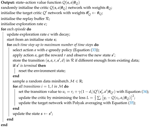
Figure 1 shows an AUV attempting to dock onto a platform. For simplicity, the problem is constrained to the vertical plane, with motions limited to surge, heave and pitch. Furthermore, the effects from currents are neglected. Let us define the vector of generalised coordinates in the inertial reference frame as

$$\mathit{\eta }={\left[\begin{array}{ccc}x& z& \theta \end{array}\right]}^T,$$

(1)

where x is the displacement in surge, z in heave and $\theta$ the pitch angle, and the vector of generalised coordinate rates in the body-fixed frame as

$$\mathit{\nu }={\left[\begin{array}{ccc}u& w& q\end{array}\right]}^T,$$

(2)

where u and w are the components of the absolute velocity of the centre of buoyancy in the body-fixed frame in surge and heave, respectively, and q is the pitch rate (identical in the inertial and body-fixed frames, since the analysis is planar). Note that, as shown in Figure 1, a right-hand reference system is employed, with the z-axis being positive downwards, as is standard practice [33]. It is possible to show that the velocity of the AUV in the inertial reference frame is given by the following relation [33]:

$$\dot{\mathit{\eta }}=\mathit{J}\left(\mathit{\eta }\right)\mathit{\nu },$$

(3)

where the transformation matrix is

$$\mathit{J}\left(\mathit{\eta }\right)=\left[\begin{array}{ccc}cos\theta & sin\theta & 0\\ -sin\theta & cos\theta & 0\\ 0& 0& 1\end{array}\right].$$

(4)

Here, the AUV is assumed to be torpedo-shaped, so that is actuated by a propeller and a sternplane. Additionally, the centres of gravity and buoyancy are assumed to be vertically in line to avoid trim angles, but the centre of gravity is lower to provide hydrostatic stability. Therefore, it is possible to show that the velocity vector of the AUV in the body-fixed frame can be expressed with the following system of nonlinear equations [24,33]:

$$\dot{\mathit{\nu }}={\mathit{M}}^{-1}\mathit{f}(\mathit{\eta },\mathit{u}),$$

(5)

where the input vector is

$$\mathit{u}={\left[\begin{array}{cc}{Q}_{\mathrm{m}}& {\delta }_{\mathrm{s}}\end{array}\right]}^T,$$

(6)

with $Q_{\mathrm{m}}$ being the motor torque and ${\delta }_{\mathrm{s}}$ the sternplane angle. The mass matrix is expressed as

$$\mathit{M}=\left[\begin{array}{ccc}(m-X_{\dot{u}})& 0& m{z}_{\mathrm{g}}\\ 0& (m-Z_{\dot{w}})& -Z_{\dot{q}}\\ m{z}_{\mathrm{g}}& -M_{\dot{w}}& (I_{yy}-M_{\dot{q}})\end{array}\right]$$

(7)

and the nonlinear vector

$$\mathit{f}(\mathit{\eta },\mathit{u})=\left[\begin{array}{c}-(W-B)sin\theta +X_{u\left|u\right|}u\left|u\right|+(X_{wq}-m)wq+X_{qq}{q}^2+(1-{\tau }_{\mathrm{p}})T_{n\left|n\right|}n\left|n\right|\\ (W-B)cos\theta +Z_{uw}uw+(Z_{uq}+m)uq+Z_{w\left|w\right|}w\left|w\right|+Z_{q\left|q\right|}q\left|q\right|+m{z}_{\mathrm{g}}{q}^2+Z_{uu{\delta }_{\mathrm{s}}}{u}^2{\delta }_{\mathrm{s}}\\ -W{z}_{\mathrm{g}}sin\theta +M_{uw}uw+M_{uq}uq+M_{w\left|w\right|}w\left|w\right|-m{z}_{\mathrm{g}}wq+M_{q\left|q\right|}q\left|q\right|+M_{uu{\delta }_{\mathrm{s}}}{u}^2{\delta }_{\mathrm{s}}\end{array}\right].$$

(8)

The physical meaning of the hydrodynamic and hydrostatic coefficients in these equations is explained in [24,33], to which the reader is referred. Additionally, the work of Hall and Anstee [24] contains the numerical values for the coefficients for the REMUS-100 AUV, which are reported in Appendix A for completeness.

The equations of motion for a torpedo-shaped AUV are completed by the dynamic equations for the propulsion units, which include an equation for the propeller revolutions, n, and an equation for the surge velocity in the propeller plane due to wake effects, $u_{\mathrm{p}}$ [24]:

$$\begin{array}{c}\hfill \dot{n}=\frac{Q_{\mathrm{m}}-K_{n}n-Q_{n\left|n\right|}n\left|n\right|}{J_{\mathrm{m}}},\end{array}$$

(9a)

$$\begin{array}{c}\hfill {\dot{u}}_{\mathrm{p}}=\frac{T_{n\left|n\right|}n\left|n\right|-d_{\mathrm{l}}{u}_{\mathrm{p}}-d_{\mathrm{q}}\left|u_{\mathrm{p}}\right|\left[u_{\mathrm{p}}-(1-w_{\mathrm{p}})u\right]}{m_{\mathrm{f}}}.\end{array}$$

(9b)

Similar to the hydrodynamic coefficients, the model parameters can be found in Appendix A.

By merging Equations (3), (5), (9a) and (9b), it is possible to express the dynamic model of the AUV through a system of nonlinear, ordinary differential equations:

$$\dot{\mathit{x}}=\mathit{g}(\mathit{x},\mathit{u}),$$

(10)

where

$$\mathit{x}={\left[\begin{array}{cccccccc}x& z& \theta & u& w& q& n& u_{\mathrm{p}}\end{array}\right]}^T.$$

(11)

A standard integration scheme can then be employed to solve the equations in time, with a fixed-step, fourth-order-accurate Runge–Kutta scheme being used in this study [34].

2.2. Relative Motion of the AUV with Respect to the Platform

The vectors of the relative displacement and velocity of the AUV with respect to the platform can be simply expressed as

$$\begin{array}{c}\hfill {\mathit{\eta }}_{\mathrm{r}}={\mathit{\eta }}_{\mathrm{p}}-\mathit{\eta },\end{array}$$

(12a)

$$\begin{array}{c}\hfill {\dot{\mathit{\eta }}}_{\mathrm{r}}={\dot{\mathit{\eta }}}_{\mathrm{p}}-\dot{\mathit{\eta }}=-\dot{\mathit{\eta }}\end{array}$$

(12b)

for a fixed platform with state vector ${\mathit{\eta }}_{\mathrm{p}}$. In reality, the velocity vector in the body-fixed frame and the pitch angle in the inertial frame are computed from the accelerometer and gyrocompass on the AUV, whereas the relative position and velocity vectors in the inertial frame are determined from either visual or sonic sensors (with lights or beacons sited on the platform, as, for instance, described by the authors of [10,12]).

3. Classical Control of the AUV for the Docking Manoeuvre

3.1. PID Control of the Docking of the AUV

A combination of classical PID controllers and line-of-sight guidance can provide a realistic benchmark for the docking problem, as opposed to trajectory control, as described in [35]. On AUVs, it is common to have separate decoupled controllers for the surge velocity, depth and heading (yaw angle) [33], with the latter being ignored in this study because of the analysis of only motions in the vertical plane. Surge can be controlled by modifying the motor torque. Conversely, since the AUV considered here does not have side thrusters, depth can only be controlled through the sternplane angle. As a result, line-of-sight guidance can be used to determine the desired pitch angle to move the AUV to the target depth. A further controller can then change the sternplane angle to match the desired angle.

As shown in Figure 2, two controllers are employed: one to control the surge speed in the body-fixed frame and one to control the pitch angle. The desired speed is calculated with the simple formula

$$u_{\mathrm{d}}=0.5u_0\left[1+tanh\left(e_x-x_{\mathrm{d}}\right)\right],$$

(13)

where $u_0$ indicates the speed at the start of the docking manoeuvre (as defined by a fixed distance from the docking platform), $e_x=x_{\mathrm{r}}$ is the relative horizontal distance of the AUV from the platform and $x_{\mathrm{d}}$ is an arbitrary parameter that needs tuning and that is used to help the AUV slow down before reaching the platform. Similarly, line of sight-guidance is used to obtain the desired pitch angle:

$${\theta }_{\mathrm{d}}=arctan\left(\frac{e_z}{z_{\mathrm{d}}}\right),$$

(14)

where $e_z=z_{\mathrm{r}}$ is the relative vertical distance of the AUV from the platform and $z_{\mathrm{d}}$ is an arbitrary parameter that needs tuning and that is used to help the AUV turn by looking ahead. Lower values result in more aggressive manoeuvres.

The PID controllers then apply a control signal that is given by

$$u=k_{\mathrm{p}}e+k_{\mathrm{i}}{\int }_0^{t}e\left(\tau \right)\mathrm{d}\tau +k_{\mathrm{d}}\dot{e},$$

(15)

where e indicates the error signal of interest [33]. The proportional term adjusts the control signal based on the current value of the error, while the derivative term takes into account expected future variations of the error and the integral term corrects for steady-state errors by looking at past values of the error.

Furthermore, the values of the torque and sternplane angles are limited within saturation blocks to prevent them from exceeding realistic physical constraints:

$$\begin{array}{c}\hfill Q_{\mathrm{m},\min }\le Q\le Q_{\mathrm{m},\max },\end{array}$$

(16a)

$$\begin{array}{c}\hfill {\delta }_{\mathrm{s},\min }\le {\delta }_{\mathrm{s}}\le {\delta }_{\mathrm{s},\max }.\end{array}$$

(16b)

Finally, the PID controller is turned off and the simulation stopped when the vehicle is close enough to the docking point, i.e., when

$$x_{\mathrm{r}}^2+z_{\mathrm{r}}^2+{\theta }_{\mathrm{r}}^2<l_{\eta },$$

(17)

where $l_{\eta }$ is a measure of the prescribed docking accuracy.

3.2. Optimal Control of the Docking of the AUV

A parametric optimal control approach is used to find the time-dependent control input vector $\mathit{u}$ that minimises a cost function over a predefined time interval [36]. Examples for the application of parametric optimal control to nonlinear systems can be found in [37,38,39], from which this article takes inspiration. The aim is to have the AUV reach the desired docking position, orientation and velocity,

$${\mathit{x}}_{\mathrm{f}}={\left[\begin{array}{cccccccc}{x}_{\mathrm{f}}& z_{\mathrm{f}}& {\theta }_{\mathrm{f}}& u_{\mathrm{f}}& w_{\mathrm{f}}& q_{\mathrm{f}}& \mathrm{free}& \mathrm{free}\end{array}\right]}^T,$$

(18)

at the end time, $t_{\mathrm{f}}$. Note that no end condition is imposed on n and $u_{\mathrm{p}}$. Similarly, initial conditions on the states have to be specified for time $t_0=0$ s:

$${\mathit{x}}_0={\left[\begin{array}{cccccccc}{x}_0& z_0& {\theta }_0& u_0& w_0& q_0& n_0& u_{\mathrm{p},0}\end{array}\right]}^T.$$

(19)

The end condition represents the state of the AUV before starting the docking manoeuvre, i.e., when it is near the docking platform. Additionally, the control action is constrained within physical limits ${\mathit{u}}_{\min }$ and ${\mathit{u}}_{\max }$, which are due to the maximum magnitude of the torque that can be delivered by the motor and the maximum magnitude of the sternplane angle to prevent stall.

Although it is possible to form the necessary conditions whose two-point boundary value problem solution should yield the optimal trajectory, the necessary conditions for optimality result in a two-point boundary value problem whose solution is the optimal trajectory in surge, heave and pitch [36]. However, no solution was found for the docking problem due to the nonlinear and cross-coupling terms in the dynamic equations and the constraints imposed on the optimisation.

Therefore, a direct, parametric sub-optimal solution has been sought instead [36]. With this approach, the constraints were removed and included as quadratic penalty terms in the cost function instead. Fixing the end time $t_{\mathrm{f}}$ and the time step used in the computation of the cost function greatly reduces the complexity of the problem and improves the robustness of the solution. Additionally, the control input signals, i.e., the motor torque $Q_{\mathrm{m}}$ and sternplane angle ${\delta }_{\mathrm{s}}$, are represented parametrically through predefined curves. This enables the solver to find a solution, since it reduces the number of unknowns from the number of time steps to the much smaller number of parameters. Although constraints or saturation limits cannot be imposed on the control signals, a cost should be imposed on their magnitude to prevent the controller from selecting unrealistically high values.

The solution from the PID control was used to provide a more appropriate starting point to guide selection of the shape functions to parameterise the control signals for the motor torque and sternplane angle of Equation (6), respectively:

$$\begin{array}{c}\hfill Q_{\mathrm{m}}=p_1(1-tanh(t-p_2))+p_{3}exp\left[-{\left(\frac{t-p_4}{p_5}\right)}^2\right],\end{array}$$

(20a)

$$\begin{array}{c}\hfill {\delta }_{\mathrm{s}}=\sum _{i=1}^4{p}_{5+i}sin\left(\frac{i\pi t}{t_{\mathrm{f}}}\right),\end{array}$$

(20b)

where $\mathit{p}\in {\mathbb{R}}^9$ is the vector of parameters. In Equation (20b), the sternplane signal is modelled as the sum of four sinusoidal basis functions. Conversely, Equation (20a) is more heavily engineered, as it presents the sum of a hyperbolic tangent and a Gaussian function. The hyperbolic tangent creates a smoothly decaying signal, while the Gaussian function creates the dip (for $p_3<0$) shown by the PID control response in Section 5 when the motor torque inverts its direction to break the vehicle’s forward motion. A more general approach can be found in [40]. Adopting the proposed basis functions and replacing the time independent variable with a trajectory signal can result in a neater expression with fewer parameters. However, this will be the scope of future work.

The optimal control problem is thus defined as follows:

$$\underset{\mathit{u}}{min}J=0.5\left\{{\sum }_{i=1}^6{\omega }_{x,i}{\left[x_i\left(t_{\mathrm{f}}\right)-x_{\mathrm{f}}\right]}^2+{\int }_0^{t_{\mathrm{f}}}{\sum }_{j=1}^2{\omega }_{u,j}{\left[u_j(t,\mathit{p})\right]}^2\mathrm{d}t+{\omega }_{Q,0}{\left[Q_{\mathrm{m}}(t_0,\mathit{p})-Q_{\mathrm{m},0}\right]}^2+{\omega }_{Q,\mathrm{f}}{Q}_{\mathrm{m}}{(t_{\mathrm{f}},\mathit{p})}^2\right\},$$

(21)

where ${\mathit{\omega }}_x$, ${\mathit{\omega }}_u$, ${\omega }_{Q,0}$ and ${\omega }_{Q,\mathrm{f}}$ are weight terms. The last two terms of Equation (21) ensure that the motor torque signal has an initial value close to $Q_{\mathrm{m},0}$, i.e., the value of the motor torque in steady-state before initiating the docking manoeuvre, and a final value close to 0 Nm at the docking point. The dynamic equations are solved in time using Equation (10) for each computation of the cost function (21).

4. Reinforcement Learning Control of the AUV for the Docking Manoeuvre

4.1. Reinforcement Learning Statement

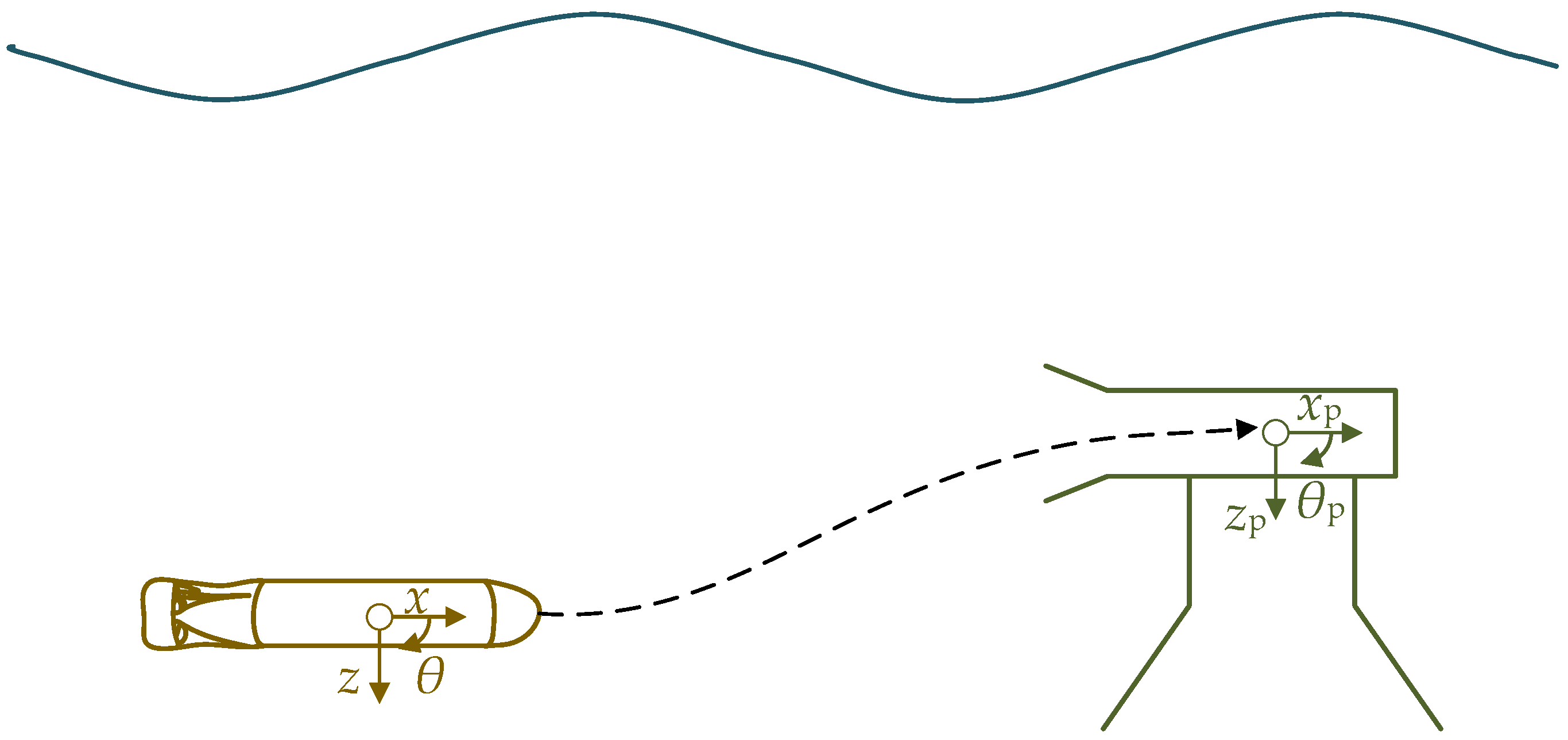
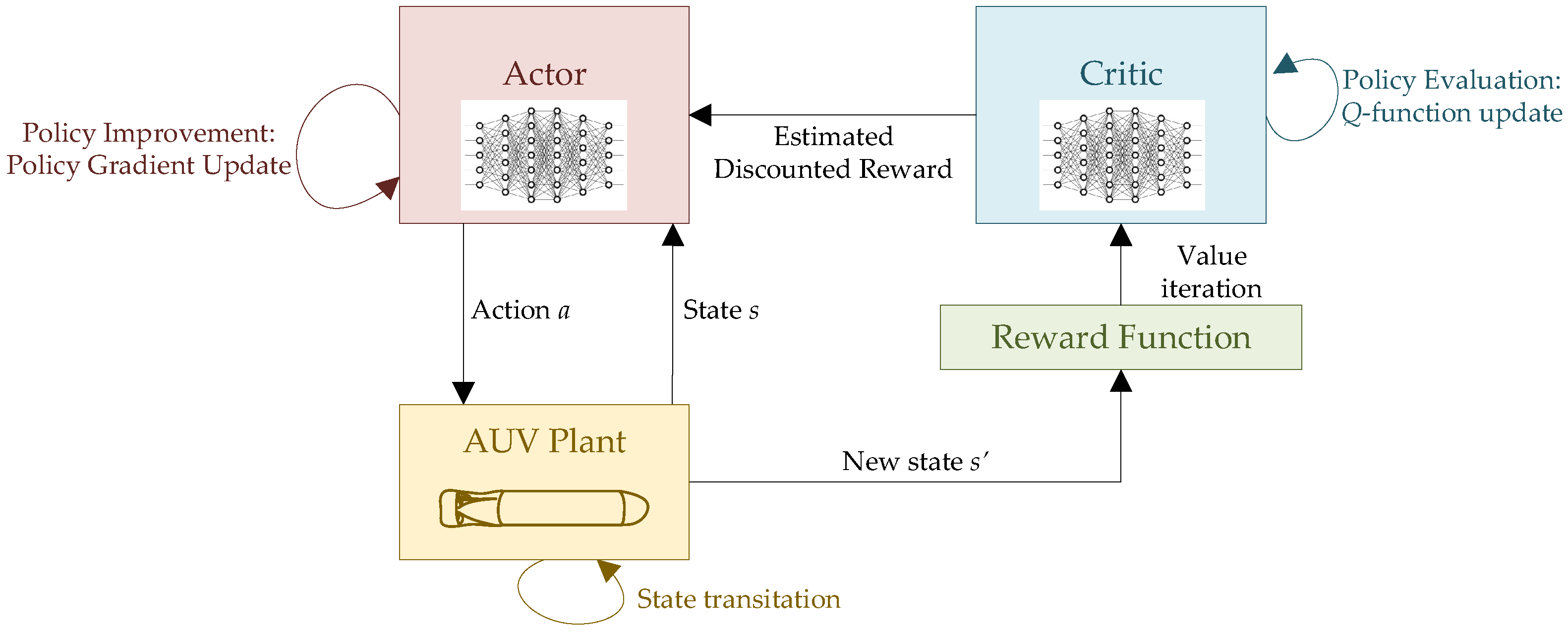
RL is a decision-making framework in which an agent learns a desired behaviour, or policy $\pi$, from direct interactions with the environment [41]. At each time step, the agent is in a states and takes and actiona. As a result, it lands in a new state $s^{\prime }$ while receiving a rewardr. A Markov decision process is used to model the action selection depending on the value function $Q(s,a)$, which represents an estimate of the future reward. By interacting the environment for a long time, the agent learns an optimal policy, which maximises the total expected reward. This is shown graphically in Figure 3.

The on-policy action-value function $Q^{\pi }(s,a)$ yields the expected reward if the agent starts in state s, takes an action a and afterwards acts according to policy $\pi$ [41]:

$$Q^{\pi }(s,a)=E_{\tau \sim \pi }\left[\sum _{t=0}^{\infty }{\gamma }^t{r}_t|s_0=s\right],$$

(22)

where $\tau =(s_0,a_0,s_1,a_1,\cdots )$ indicates a sequence of actions and states, $\gamma \in [0,1]$ is a discount factor and E expressed the expected, discounted value. Conversely, the optimal action-value function $Q^{*}(s,a)$ yields the expected reward if the optimal policy is followed after starting from state s and taking action a

$$Q^{*}(s,a)=\underset{\pi }{max}{E}_{\tau \sim \pi }\left[\sum _{t=0}^{\infty }{\gamma }^t{r}_t|s_0=s\right].$$

(23)

Since the optimal policy will result in the selection of the action that maximises the expected reward starting from s, it is possible to obtain the optimal action $a^{*}\left(s\right)$ from $Q^{*}$ as follows:

$$a^{*}\left(s\right)=\arg \underset{a}{max}{Q}^{*}(s,a).$$

(24)

As a result, it is possible to express the Bellman equation for the optimal action-value function as follows [41]:

$$Q^{*}(s,a)=E_{s^{\prime }\sim P}\left[r(s,a)+\gamma \underset{a^{\prime }}{max}{Q}^{*}(s^{\prime },a^{\prime })\right],$$

(25)

where P indicates state transitions according to a stochastic policy $\pi$.

RL algorithms can be subdivided into model-based and model-free schemes [42]. Whereas model-based strategies enable the agent to plan by exploiting the model of the environment, thus greatly improving their behaviour, exact models of the environment are generally unavailable in practice. Any existing bias in the model is likely to cause significant problems with generalising the agent’s behaviour to the actual environment. As a result, RL research has focused on model-free approaches to date.

Within model-free schemes, RL algorithms can be further categorised based on what they learn. On the one hand, the strategies in the policy optimisation group directly represent the policy and optimise its parameters. Since the policy update only relies on data collected while following the policy, these approaches are known as on-policy. Note that policies can be stochastic, defined as $\pi$, or deterministic, defined as $\mu$. On the other hand, Q-learning strategies learn an approximation for the optimal action-value function based on the Bellman equation. As the update of the optimal Q-value may employ data collected at any point during training, these schemes are known as off-policy. Whereas policy optimisation schemes are more robust, since they directly optimise what is being sought, Q-learning methods can be significantly more sample-efficient when they work.

Additionally, RL algorithms can be subdivided into on-line and off-line types. With on-line schemes, learning occurs in real time from the data stream. In off-line strategies, the policy is updated only at regular intervals and stored in memory. Both types of algorithms have much lower computational cost at deployment time than during training.

The first RL algorithms dealt with discretised state and action spaces [41]. Subsequently, linear features were introduced to approximate the state space to enable the treatment of complex control problems [43]. More recently, deep neural networks have been shown to provide better generalisation and improved learning, allowing scientists to develop systems capable of outperforming humans in complex games [44]. However, only recently have deep neural network been used to approximate the action selection process, thus enabling the inclusion of continuous action signals in the RL framework, which are typical of realistic control problems [45].

4.2. Problem Formulation

RL has been successfully applied to control applications (e.g., see, [43,46,47]). In these tasks, the controller represents the agent, while the system plant corresponds to the environment. The control output is the action, whereas the observable and estimated states may represent the state. The reward is typically expressed through a cost function. Most applications of RL to control tasks to date refer to episodic problems, i.e., the task can be defined as an episode with a specific desired outcome signalling its completion. Expressing the control problem as an episodic task greatly reduces the problem formulation complexity, as it enables the designer to exploit the classical RL framework.

For the specific application to the docking of the AUV onto a fixed platform in surge, heave and pitch, it is possible to define the RL state space as follows:

$$\mathit{s}={\left[\begin{array}{ccccccc}{x}_{\mathrm{r}}& z_{\mathrm{r}}& {\theta }_{\mathrm{r}}& \dot{x}& \dot{z}& \dot{\theta }& n\end{array}\right]}^T.$$

(26)

It is necessary to add the propeller revolutions, n, to the state-space to provide an indication of the propeller thrust. Changes in motor torque will affect the thrust, but with a delay. Hence, ideally, the controller should learn to reduce the propeller revolutions as it approaches the goal position and orientation. Similarly, the action space is identical to the control output $\mathit{u}$:

$$\mathit{a}=\mathit{u}={\left[\begin{array}{cc}{Q}_{\mathrm{m}}& {\delta }_{\mathrm{s}}\end{array}\right]}^T.$$

(27)

However, to prevent stall and because of torque limitations, the selected continuous action should be constrained to minimum and maximum values (${\mathit{a}}_{\min }$ and ${\mathit{a}}_{\max }$, respectively).

Specifying an appropriate reward function is fundamental to have the agent learn the desired behaviour. Although it is possible to inverse-engineer reward functions from examples or expert pilots [48], here a reward function is designed similarly to cost functions for control problems. In particular, the reward function for the docking problem should comprise of different elements: a continuous cost on the action to limit excessive power expenditures, a continuous cost on position so that the AUV is guided towards the docking point, a continuous cost on velocity so that small terminal speed is achieved, a high penalty for exceeding realistic environmental boundaries and high rewards once the AUV is close enough to docking point and at low speeds. The penalty and rewards make the reward function discontinuous and reliant on an if-loop. Inspiration for the reward function is taken from [32], where the authors employed RL for the landing of a spacecraft. Similarly, the cost on the velocity is expressed as a function of the distance to the desired docking point. This is because at low speeds the sternplane becomes ineffective due to the drop in lift force. Hence, a higher speed away from the docking point is necessary to achieve the desired level of control. Therefore, the reward function that has been designed for the docking of an AUV to a fixed or moving platform is

$$c=-{\omega }_x{x}_{\mathrm{r}}^2-{\omega }_z{z}_{\mathrm{r}}^2-{\omega }_{\theta }{\theta }_{\mathrm{r}}^2-{\omega }_Q{Q}_{\mathrm{m}}^2-{\omega }_{{\delta }_{\mathrm{s}}}{\delta }_{\mathrm{s}}^2-{\omega }_u\frac{u^2}{max(x_{\mathrm{r}}^2,l_u)},$$

(28)

$$r=\left\{\begin{array}{}\mathrm{(29a)}& \begin{array}{cc}c\hfill & \mathrm{if} f=0 \mathrm{and} h=0,\hfill \end{array}\hfill \mathrm{(29b)}& \begin{array}{cc}-p\hfill & \mathrm{if} h=1,\hfill \end{array}\hfill \mathrm{(29c)}& \begin{array}{cc}c+r_{\mathrm{f}}+\frac{{\omega }_{\dot{x}}}{max({\dot{x}}_{\mathrm{r}}^2,l_{\dot{x}})}+\frac{{\omega }_{\dot{z}}}{max({\dot{z}}_{\mathrm{r}}^2,l_{\dot{z}})}+\frac{{\omega }_{\dot{\theta }}}{max({\dot{\theta }}_{\mathrm{r}}^2,l_{\dot{\theta }})}\hfill & \mathrm{if} f=1.\hfill \end{array}\hfill \end{array}\right.$$

The constants $\omega$ indicate weights and l limiting values. The parameter $r_{\mathrm{f}}$ is an additional reward achieved at the end of the episode for successful docking. Note that f is a boolean that expresses whether docking is achieved to the desired level of accuracy:

$$f=\left\{\begin{array}{}\mathrm{(30a)}& \begin{array}{cc}1\hfill & \mathrm{if} x_{\mathrm{r}}^2+z_{\mathrm{r}}^2+{\theta }_{\mathrm{r}}^2<l_{\eta },\hfill \end{array}\hfill \mathrm{(30b)}& \begin{array}{cc}0\hfill & \mathrm{if} x_{\mathrm{r}}^2+z_{\mathrm{r}}^2+{\theta }_{\mathrm{r}}^2\ge l_{\eta }.\hfill \end{array}\hfill \end{array}\right.$$

Additionally, the boolean h describes whether the episode should be terminated because the AUV exceeds sensible environmental boundaries:

$$h=\left\{\begin{array}{}\mathrm{(31a)}& \begin{array}{cc}1\hfill & \mathrm{if} x_{\mathrm{r}}>l_{x,\max } \mathrm{or} x_{\mathrm{r}}<l_{x,\min } \mathrm{or} z_{\mathrm{r}}>l_{z,\max } \mathrm{or} z_{\mathrm{r}}<l_{z,\min } \mathrm{or} {\theta }_{\mathrm{r}}>l_{\theta ,\max } \mathrm{or} {\theta }_{\mathrm{r}}<l_{\theta ,\min },\hfill \end{array}\hfill \mathrm{(31b)}& \begin{array}{cc}0\hfill & \mathrm{otherwise}.\hfill \end{array}\hfill \end{array}\right.$$

The limiting values as well as the weights and other parameters in the reward function need to be tweaked until the desired performance is achieved. In particular, a compromise needs to be found between docking time, accuracy and the end speed. The boolean variables f and h are combined into an additional variable d that determines whether the episode ends:

$$d=\left\{\begin{array}{}\mathrm{(32a)}& \begin{array}{cc}1\hfill & \mathrm{if} f=1 \mathrm{or} h=1,\hfill \end{array}\hfill \mathrm{(32b)}& \begin{array}{cc}0\hfill & \mathrm{otherwise}.\hfill \end{array}\hfill \end{array}\right.$$

d is used in the following section to determine the RL algorithm behaviour.

4.3. Deep Q-Network

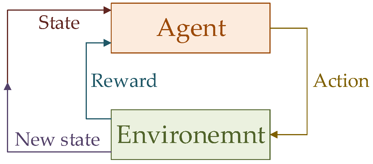
The first RL algorithm investigated is deep Q-network (DQN), a popular model-free, on-line, off-policy strategy [44,49]. DQN trains a critic to approximate the action-value (or Q-) function $Q(\mathit{s},a|{\mathit{\theta }}_Q)$, i.e., to estimate the return of future rewards. Hence, the algorithm relies on a discrete action-space and a continuous state-space. As a result, the action is selected with an $ϵ$-greedy policy [41]:

$$a=\left\{\begin{array}{}\mathrm{(33a)}& \begin{array}{cc}\arg \underset{a^{\prime }\in \mathcal{A}}{max}Q(\mathit{s},a^{\prime }|{\mathit{\theta }}_Q)\hfill & \mathrm{if} b\le ϵ,\hfill \end{array}\hfill \mathrm{(33a)}& \begin{array}{cc}\mathrm{random}(a^{\prime }\in \mathcal{A})\hfill & \mathrm{if} b>ϵ,\hfill \end{array}\hfill \end{array}\right.$$

where $\mathcal{A}$ indicates the action space, i.e., a vector of all possible actions, $b\in [0,1]$ is a random number and $ϵ\in [0,1]$ is defined as the exploration rate. The exploration rate is typically set to a high value close to 1 at the start of the training process and as learning progresses a decay function is employed to lower its value. This ensures that the agent focuses on exploring the environment at the beginning and then shifts to exploiting the optimal actions as learning progresses.

In DQN, the critic approximator is represented by a deep neural network. Two features ensure that training occurs smoothly. Firstly, the algorithm relies on the concepts of experience replay buffer [44,45]. With this strategy, at each step, the state state, action, reward, new state and flag for episode end from the previous step $(\mathit{s},\mathit{a},r,{\mathit{s}}^{\prime },d)$ are saved as a transition inside the experience memory buffer $\mathcal{R}$. During training, a mini-batch of experiences $\mathcal{M}\in \mathcal{R}$ is then sampled from the memory to update the deep neural networks. If only the latest experience is used, the neural network is likely to suffer from overfitting. To ensure stability, the replay buffer should be large and contain data from a wide range for each variable. However, only a limited number of data points (usually in the order of ${10}^6$–${10}^7$) can be stored in memory. Hence, new experience should be stored only if it describes a data point different enough from the existing data. Furthermore, using batches sampled randomly from the experience buffer ensures the best compromise between computational performance and overfitting avoidance. Since learning occurs without relying on the current experience, DQN is described as off-policy scheme.

Furthermore, the DQN algorithm exploits the concept of a target network for the critic to improve learning and enhance the stability of the optimisation. This network, $Q^{\prime }(\mathit{s},a|{\mathit{\theta }}_Q^{\prime })$ has the same structure and parameterisation as $Q(\mathit{s},a|{\mathit{\theta }}_Q)$. The value function target is thus set as

$$y=r+\gamma (1-d)\underset{a^{\prime }\in \mathcal{A}}{max}{Q}^{\prime }({\mathit{s}}^{\prime },a^{\prime }|{\mathit{\theta }}_{Q^{\prime }}),$$

(34)

which indicates the sum of the immediate and discounted future reward. The main problem is that the value function target depends on the same parameters that are being learned in training, thus making the minimisation of the mean-squared Bellman error unstable. For this reason, the target network is used, as it has the same set of parameters are the critic network, but lags it in time. Hence, the target network is updated once per main network update by Polyak averaging [45]:

$${\theta }_{Q^{\prime }}=\tau {\theta }_Q+(1-\tau ){\theta }_{Q^{\prime }},$$

(35)

where $\tau \in [0,1]$ is the smoothing factor.

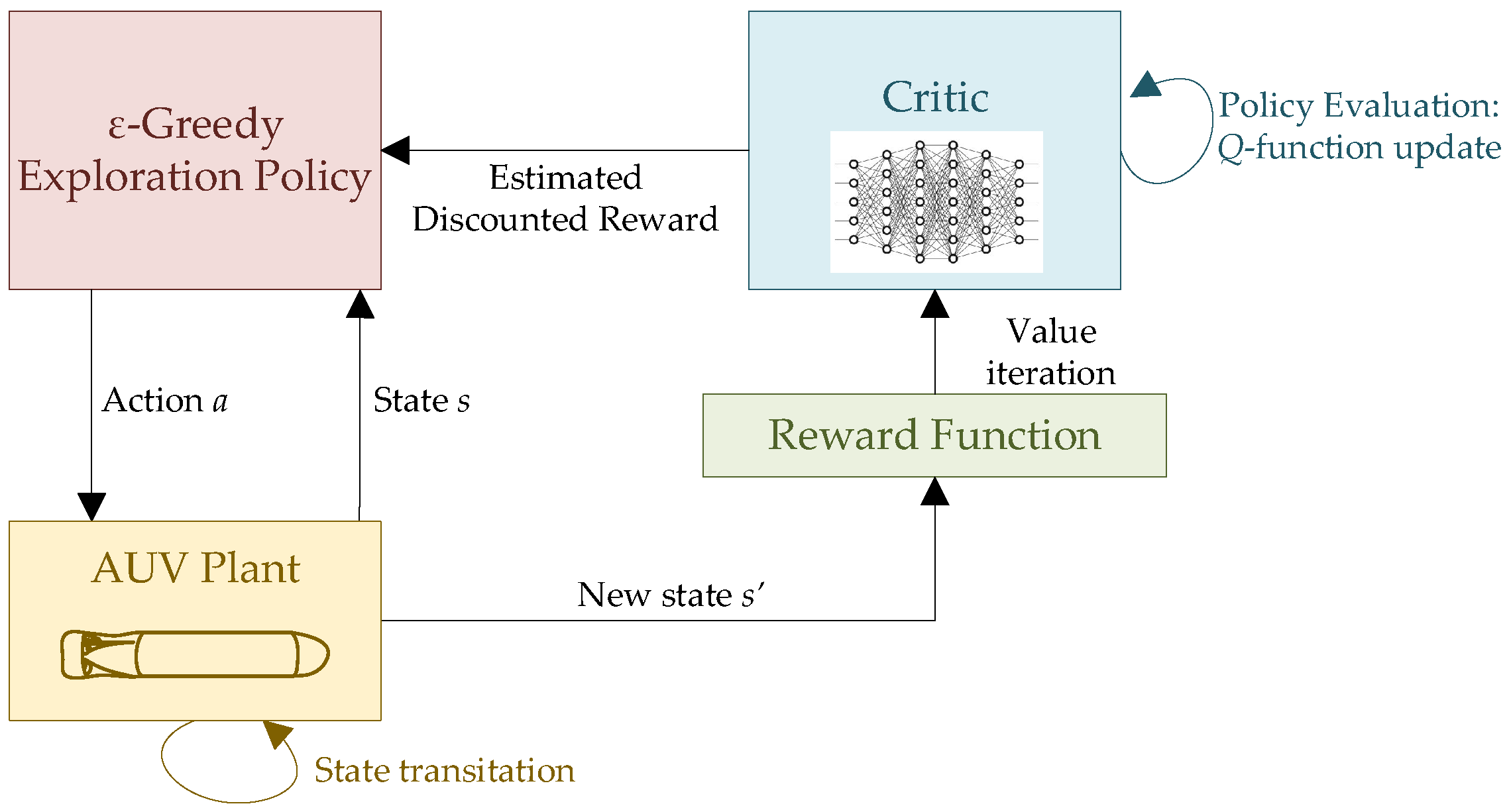
The DQN algorithm is summarised in Algorithm 1, which is taken from [44,49] with the addition of Polyak averaging as in the MATLAB implementation used here.

DQN Docking Control of an AUV in 3 DOF

Since DQN relies on discrete actions, only a limited set of actions $\mathcal{A}$ can be selected by the controller. One common approach with RL schemes with discrete actions is to select three actions per action signal: the maximum, minimum and zero values of the signal [43]. This results in a bang-bang control type, which can be proven to be optimal with Pontryagin’s principle [36]. However, here, a different approach is selected similarly to [50,51].

The action space is selected as the combination of positive, negative and zero step changes in the motor torque and sternplane angle, as described in Section 5.1. Therefore, at each time step, the motor torque and sternplane angle are changed by a fixed amount, which should be selected as a realistic value based on the physical constraints of the system. To ensure learning occurs, the values of $Q_{\mathrm{m}}$ and ${\delta }_{\mathrm{s}}$ must be tracked. Otherwise, the action information, i.e., a relative change in the control input, is not sufficient for the agent to successfully learn a policy, since information on the absolute (positive or negative) value of the motor torque and sternplane angle is required. Hence, the state space in Equation (26) is modified as follows for the DQN algorithm for the docking control of the AUV in 3 DOF:

$${\mathit{s}}_{\mathrm{DQN}}={\left[\begin{array}{ccc}\mathit{s}& Q_{\mathrm{m}}& {\delta }_{\mathrm{s}}\end{array}\right]}^T.$$

(36)

Note that upper and lower limits are imposed on the values of the motor torque and sternplane angles to reflect realistic physical boundaries. Hence, even if the action corresponding to a positive change in motor torque is selected for $Q_{\mathrm{m}}=Q_{\mathrm{m},\max }$, no changes will be applied, since the value of $Q_{\mathrm{m}}$ is saturated.

Algorithm 1: DQN algorithm adapted from [49].

The DQN aglorithm for the docking control of the AUV onto a fixed platform in surge, heave and pitch is shown graphically in Figure 4.

4.4. Deep Deterministic Policy Gradient

A popular model-free, on-line, off-policy RL algorithm known as deep deterministic policy gradient (DDPG) is adopted here [45]. Although DDPG has been found to be sensitive to hyperparameter tuning and to suffer from overestimating the Q-values [46,47], it has been successfully applied to the depth and low-level control of AUVs [30,31].

DDPG is a type of actor-critic strategy developed by Lillicrap et al. [45]. As shown in Figure 5, the critic evaluates the action-value (or Q-)function, while the actor improves the policy in the direction suggested by the critic. In DDPG, a deep neural network is used by the critic to approximate the expectation of the long-term reward based on the state observation $\mathit{s}$ and action $\mathit{a}$. Hence, the state–action value function can be expressed through the neural network features ${\mathit{\theta }}_Q$ as $Q(\mathit{s},\mathit{a},{\mathit{\theta }}_Q)$. An additional deep neural network is employed by the actor for the approximation of the optimal policy: based on state $\mathit{s}$, the network returns the continuous action $\mathit{a}$ that is expected to maximise the long-term reward or state–action value. Thus, by including the neural network features ${\mathit{\theta }}_{\mu }$, the policy can be expressed as $\mu (\mathit{s},{\mathit{\theta }}_{\mu })$. Hence, in the DDPG algorithm, the agent learns a deterministic policy and the Q-function concurrently.

Furthermore, similar to DQN, the DDPG algorithm exploits target networks for the critic and actor to improve learning and enhance the stability of the optimisation. These networks, $Q^{\prime }(\mathit{s},\mathit{a},{\mathit{\theta }}_Q^{\prime })$ and ${\mu }^{\prime }(\mathit{s},{\mathit{\theta }}_{\mu }^{\prime })$, respectively, have the same structure and parameterisation as $Q(\mathit{s},\mathit{a},{\mathit{\theta }}_Q)$ and $\mu (\mathit{s},{\mathit{\theta }}_{\mu })$, respectively. The value function target is thus set as

$$y=r+\gamma (1-d)Q^{\prime }({\mathit{s}}^{\prime },{\mu }^{\prime }\left({\mathit{s}}^{\prime }\right|{\mathit{\theta }}_{\mu }^{\prime })|{\mathit{\theta }}_{Q^{\prime }}),$$

(37)

which indicates the sum of the immediate and discounted future reward. In Equation (37), the agent first obtains the new observation from the policy through the actor. Then, the cumulative reward is found through the critic. As for DQN, the target networks are updated once per main network updated by Polyak averaging [45] with the following equation in addition to Equation (35):

$${\theta }_{{\mu }^{\prime }}=\tau {\theta }_{\mu }+(1-\tau ){\theta }_{{\mu }^{\prime }}.$$

(38)

Similar to DQN, DDPG is an off-policy strategy as it relies on an experience replay buffer. Using the samples in the data batch $\mathcal{M}$, the parameters of the deep neural network for the critic are updated by minimising the loss over all I samples [45]:

$$L=\frac{1}{I}\sum _i{\left[y_i-Q(s_i,a_i|{\mathit{\theta }}_Q)\right]}^2.$$

(39)

Conversely, the parameter of the deep neural network for the actor are updated by maximising the expected discounted reward:

$${\nabla }_{{\mathit{\theta }}_{\mu }}J\approx \frac{1}{I}\sum _i{\nabla }_{\mathit{a}}Q(\mathit{s},\mathit{a}|{\mathit{\theta }}_Q){{|}_{\mathit{s}={\mathit{s}}_i,\mathit{a}=\mu \left({\mathit{s}}_i\right)}{\nabla }_{{\mathit{\theta }}_{\mu }}\mu \left(\mathit{s}\right|{\mathit{\theta }}_{\mu })|}_{{\mathit{s}}_i}.$$

(40)

The off-policy nature of the DDPG algorithm is further exploited to deal with the RL long-standing compromise of exploration and exploitation. Especially during the initial stages of learning, it is fundamental for the agent to explore the state–action space to optimise performance and avoid getting stuck in a local optimum. As learning progresses, the agent can focus on exploiting the action that yields maximum overall reward. Since the policy provided by the actor is deterministic, noise needs to be added to the action during training to ensure sufficient levels of exploration. Ornstein–Uhlenbeck noise is selected as in [45].

The DDPG algorithm is summarised in Algorithm 2.

Algorithm 2: DDPG algorithm adapted from [45].

5. Results

5.1. Simulation Framework

The equations of motion in Section 2 were used to simulate the dynamics of a REMUS 100 AUV in surge, heave and pitch. The model parameters for this device were taken from [24] and are included in Appendix A for completeness. Note that for simplicity zero net buoyancy was assumed here. The simulation was implemented in the MATLAB/Simulink interface using specially designed C-coded S-functions. The MATLAB fminunc optimisation function was used by the optimal controller with the Quasi-Newton optimisation algorithm [52]. A fourth-order-accurate Runge–Kutta method with fixed time step was used for the integration [53]. Although the simulation time step was set at 0.01 s to prevent numerical instabilities, the parametric optimal and the RL controllers operate with a more realistic sample period of 0.2 s. This value is a compromise between hardware limitations, power consumption and control performance. Although the sample rate was much higher than typical AUV operations, a shorter time step was required for the docking manoeuvre due to the required level of accuracy. The total simulation time was capped at 50 s (i.e., a time-out), with shorter times possible if docking occurs sooner.

The AUV starting state vector was set as

$${\mathit{x}}_0={\left[\begin{array}{cccccccc}0\mathrm{m}& 1\mathrm{m}& 0\mathrm{rad}& 1.10513\mathrm{m}/\mathrm{s}& 0\mathrm{m}/\mathrm{s}& 0\mathrm{rad}/\mathrm{s}& 80.1440\mathrm{rad}/\mathrm{s}& 0.792386\mathrm{m}/\mathrm{s}\end{array}\right]}^T,$$

(41)

which corresponds to steady-state conditions for ${\delta }_{\mathrm{s}}=0$ rad and $Q_{\mathrm{m}}=40$ Nm. The docking platform was sited at $x_{\mathrm{p}}=20$ m, $z_{\mathrm{p}}=0$ m and ${\theta }_{\mathrm{p}}=0$ rad. The measure of docking accuracy was set at $l_{\eta }=0.1$. Additionally, ideally, the desired velocity vector of the AUV at the docking pointwas set to ${\dot{x}}_{\mathrm{f}}=0.1$ m/s, ${\dot{z}}_{\mathrm{f}}=0$ m/s and ${\dot{\theta }}_{\mathrm{f}}=0$ rad/s, as these values ensure a gentle manoeuvre. To prevent stall and include realistic constraints on the motor torque, $Q_{\mathrm{m}},\max =100$ Nm, $Q_{\mathrm{m}},\min =-100$ Nm, ${\delta }_{\mathrm{s}},\max ={15}^{\circ }$ and ${\delta }_{\mathrm{s}},\min =-{15}^{\circ }$.

The discrete action space for the DQN algorithm was selected as

$$\mathcal{A}={\left[\begin{array}{ccccccccc}\delta Q_{\mathrm{m}}& 0& -\delta Q_{\mathrm{m}}& \delta Q_{\mathrm{m}}& 0& -\delta Q_{\mathrm{m}}& \delta Q_{\mathrm{m}}& 0& -\delta Q_{\mathrm{m}}\\ \delta {\delta }_{\mathrm{s}}& \delta {\delta }_{\mathrm{s}}& \delta {\delta }_{\mathrm{s}}& 0& 0& 0& -\delta {\delta }_{\mathrm{s}}& -\delta {\delta }_{\mathrm{s}}& -\delta {\delta }_{\mathrm{s}}\end{array}\right]}^T,$$

(42)

where $\delta Q_{\mathrm{m}}=10$ Nm represents the selected step change in motor torque and $\delta {\delta }_{\mathrm{s}}=3^{\circ }$ in sternplane angle.

Table 1. Parameters used by the PID controller.

${\mathit{u}}_0$ (m/s)	${\mathit{x}}_{\mathbf{d}}$ (m)	${\mathit{z}}_{\mathbf{d}}$ (m)	${\mathit{k}}_{\mathbf{p},\mathit{u}}$	${\mathit{k}}_{\mathbf{i},\mathit{u}}$	${\mathit{k}}_{\mathbf{d},\mathit{u}}$	${\mathit{k}}_{\mathbf{p},\mathit{\theta }}$	${\mathit{k}}_{\mathbf{i},\mathit{\theta }}$	${\mathit{k}}_{\mathbf{d},\mathit{\theta }}$
1.10513	10	2	100	2	4	100	2	4

,

Table 2. Parameters used by the parametric optimal controller.

${\mathit{\omega }}_{\mathit{x},1}$	${\mathit{\omega }}_{\mathit{x},2}$	${\mathit{\omega }}_{\mathit{x},3}$	${\mathit{\omega }}_{\mathit{x},4}$	${\mathit{\omega }}_{\mathit{x},5}$	${\mathit{\omega }}_{\mathit{x},6}$	${\mathit{\omega }}_{\mathit{u},1}$	${\mathit{\omega }}_{\mathit{u},2}$	${\mathit{\omega }}_{\mathit{Q},0}$	${\mathit{t}}_{\mathit{Q},\mathbf{f}}$	${\mathit{Q}}_{\mathbf{m},0}$	${\mathit{t}}_{\mathbf{f}}$
1000	1000	100	10000	100	100	0.001	0.1	500	500	40 Nm	30 s

,

Table 3. Weights used by the RL reward function.

${\mathit{\omega }}_{\mathit{x}}$	${\mathit{\omega }}_{\mathit{z}}$	${\mathit{\omega }}_{\mathit{\theta }}$	${\mathit{\omega }}_{{\mathit{Q}}_{\mathbf{m}}}$	${\mathit{\omega }}_{{\mathit{\delta }}_{\mathbf{s}}}$	${\mathit{\omega }}_{\mathit{u}}$	${\mathit{\omega }}_{\dot{\mathit{x}}}$	${\mathit{\omega }}_{\dot{\mathit{z}}}$	${\mathit{\omega }}_{\dot{\mathit{\theta }}}$	p	${\mathit{r}}_{\mathbf{f}}$
0.4	1.2	0.2	0.05	0.1	0.5	10,000	1000	500	20,000	10,000

and

Table 4. Parameters used by the RL reward function.

${\mathit{l}}_{\mathit{u}}$	${\mathit{l}}_{\dot{\mathit{x}}}$	${\mathit{l}}_{\dot{\mathit{z}}}$	${\mathit{l}}_{\dot{\mathit{\theta }}}$	${\mathit{l}}_{\mathit{x},\mathbf{min}}$	${\mathit{l}}_{\mathit{x},\mathbf{max}}$	${\mathit{l}}_{\mathit{z},\mathbf{min}}$	${\mathit{l}}_{\mathit{z},\mathbf{max}}$	${\mathit{l}}_{\mathit{\theta },\mathbf{min}}$	${\mathit{l}}_{\mathit{\theta },\mathbf{max}}$
0.05	0.01	0.01	0.01	−2 m	22 m	−4 m	4 m	−45°	45°

contain the parameters used by the PID, parametric optimal and RL controllers, respectively. For the RL algorithms, the parameters were initialised from common-sense values based on the literature (e.g., from [32]) and then tuned to achieve successful docking for the analysed cases. Furthermore, the following limits were used to normalise the state vector to help the training of the deep neural networks:

$$\begin{array}{c}\hfill {\mathit{s}}_{\min }={\left[\begin{array}{ccccccc}{l}_{x,\min }& l_{z,\min }& l_{\theta ,\min }& -2\mathrm{m}/\mathrm{s}& -1\mathrm{m}/\mathrm{s}& -2\mathrm{rad}/\mathrm{s}& -200\mathrm{rad}/\mathrm{s}\end{array}\right]}^T,\end{array}$$

(43a)

$$\begin{array}{c}\hfill {\mathit{s}}_{\max }={\left[\begin{array}{ccccccc}{l}_{x,\max }& l_{z,\max }& l_{\theta ,\max }& 2\mathrm{m}/\mathrm{s}& 1\mathrm{m}/\mathrm{s}& 2\mathrm{rad}/\mathrm{s}& 200\mathrm{rad}/\mathrm{s}\end{array}\right]}^T.\end{array}$$

(43b)

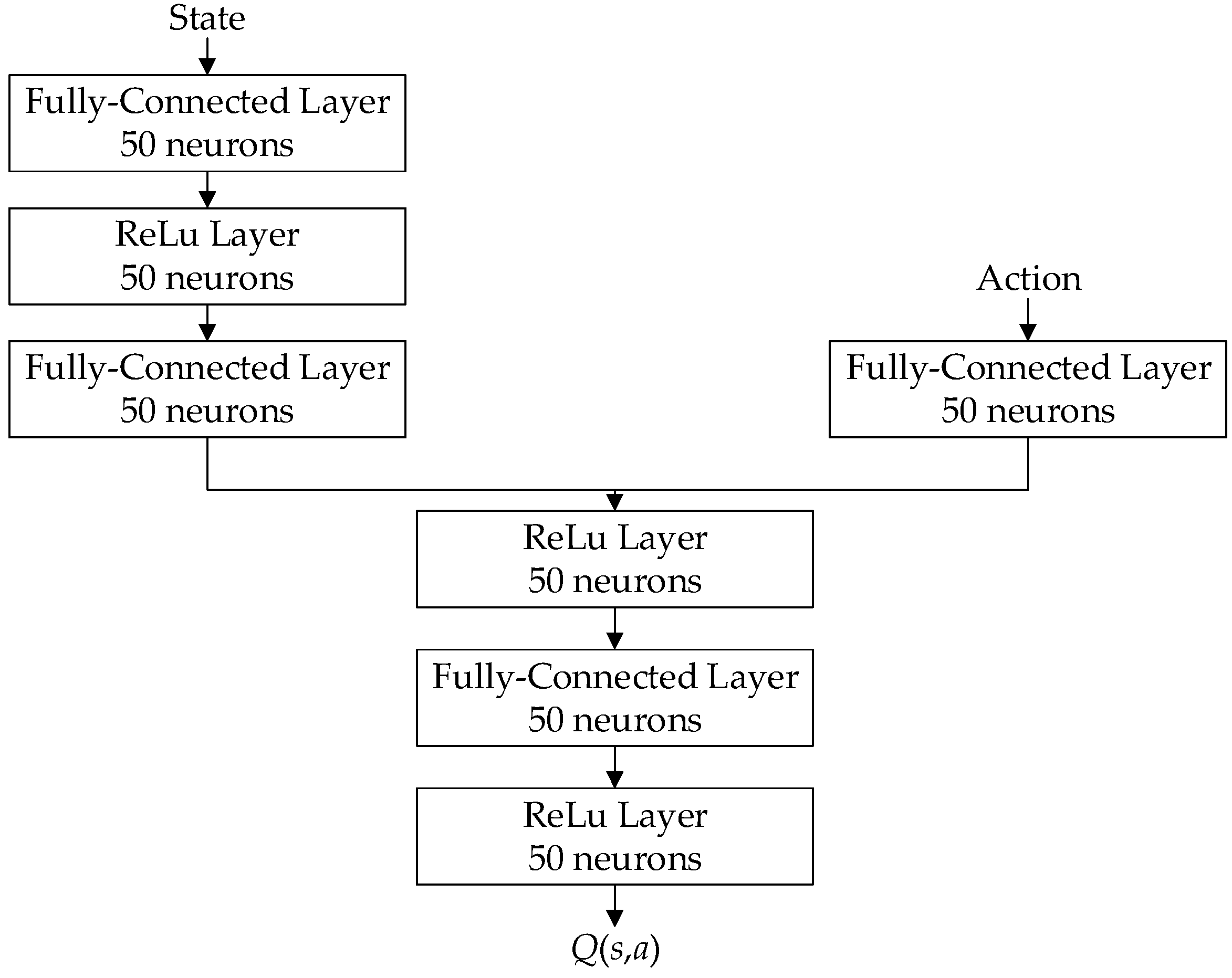
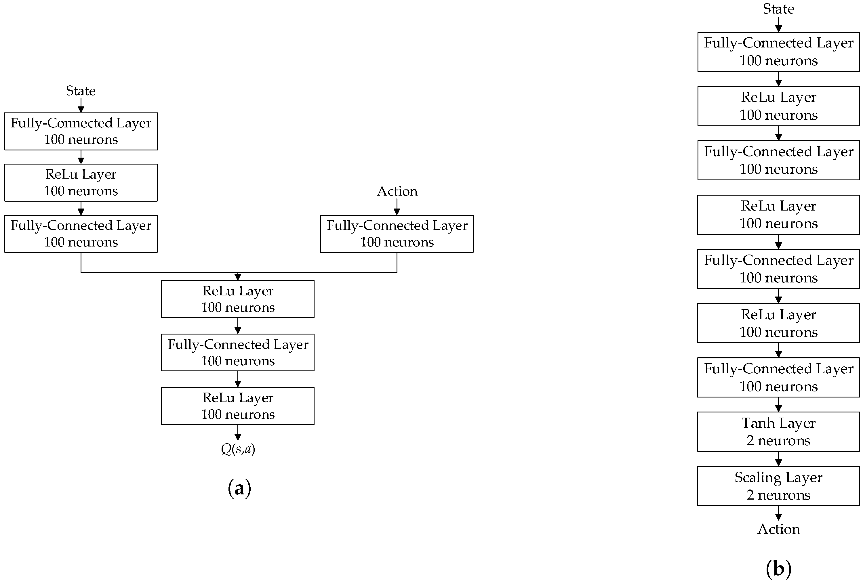
The deep neural networks used to approximate the critic for the DQN algorithm and the critic and the actor for the DDPG algorithm can be seen in Figure 6 and Figure 7, respectively. While the number of neurons was selected for optimal docking performance (out of 25, 50, 100 and 200 neurons for a single seed value), the network layout and number of layers were adopted from recommendations by Mathworks. A fully connected layer employs a linear function to multiply the input by a weight matrix and then add a bias vector. A ReLu layer employs the rectified linear unit activation function, which is the most popular type of activation function in deep neural networks nowadays. A tanh layer, which employs the hyperbolic tangent activation function, was used to constrain the action output to the range $(-1,1)$, which was then scaled back up to the desired magnitude by a linear layer. The adaptive learning rate optimisation algorithm Adam was used for training the neural networks [54]. The learning rate was set at 0.001 with a gradient threshold of 1 for both critic networks, while the actor network had a learning rate of 0.0001. The reader is referred to [55] for greater information.

Batches of 128 data samples were used for experience replay during learning. An experience buffer length of ${10}^6$ points was set to reduce the memory cost. The discount factor was set to $\gamma =0.99$ to favour learning of long-term reward. For the DQN algorithm, the initial exploration rate was set to ${ϵ}_0=1$ with a decay of 0.0001 and a minimum value of ${ϵ}_{\min }=0.01$. For the DDPG algorithm, the initial variance was set to 0.3 with a decay of 0.0001. The smoothing factor was set to $\tau =0.001$. The reinforcement learning and deep learning toolboxes of MATLAB were used to model the RL agents and deep neural networks.

5.2. Docking of an AUV onto a Fixed Platform

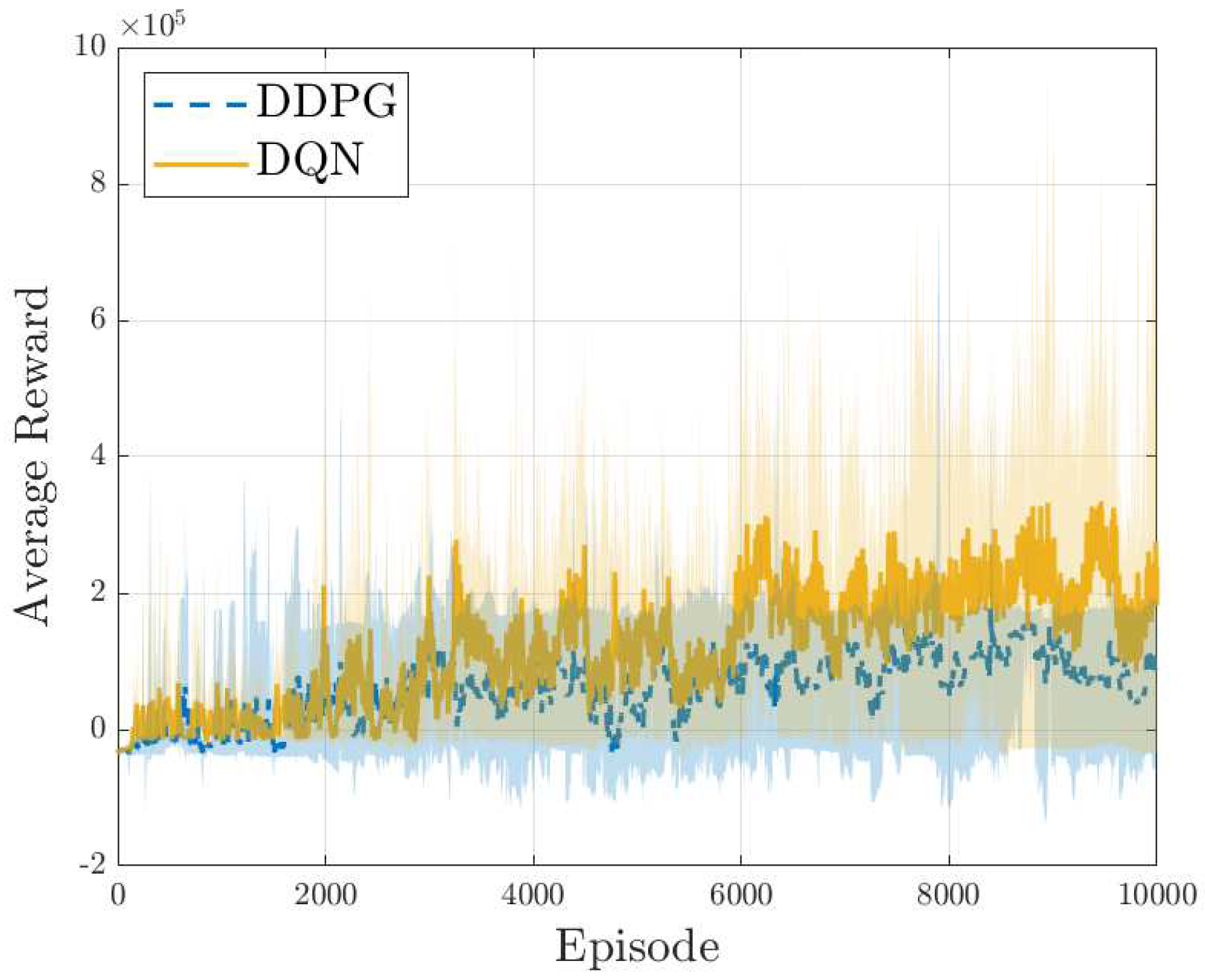
The learning behaviour of the DQN and DDPG algorithms is shown in Figure 8, which shows the convergence with episode number of the reward per episode averaged over a moving window of 10 episodes. The research was averaged over five training sessions per algorithm, initialised with different seed numbers. The shaded region indicates the values within the minimum and maximum observed average reward values.

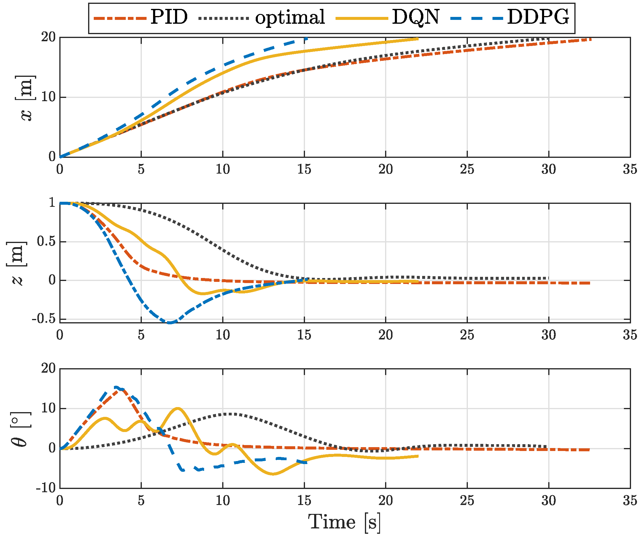
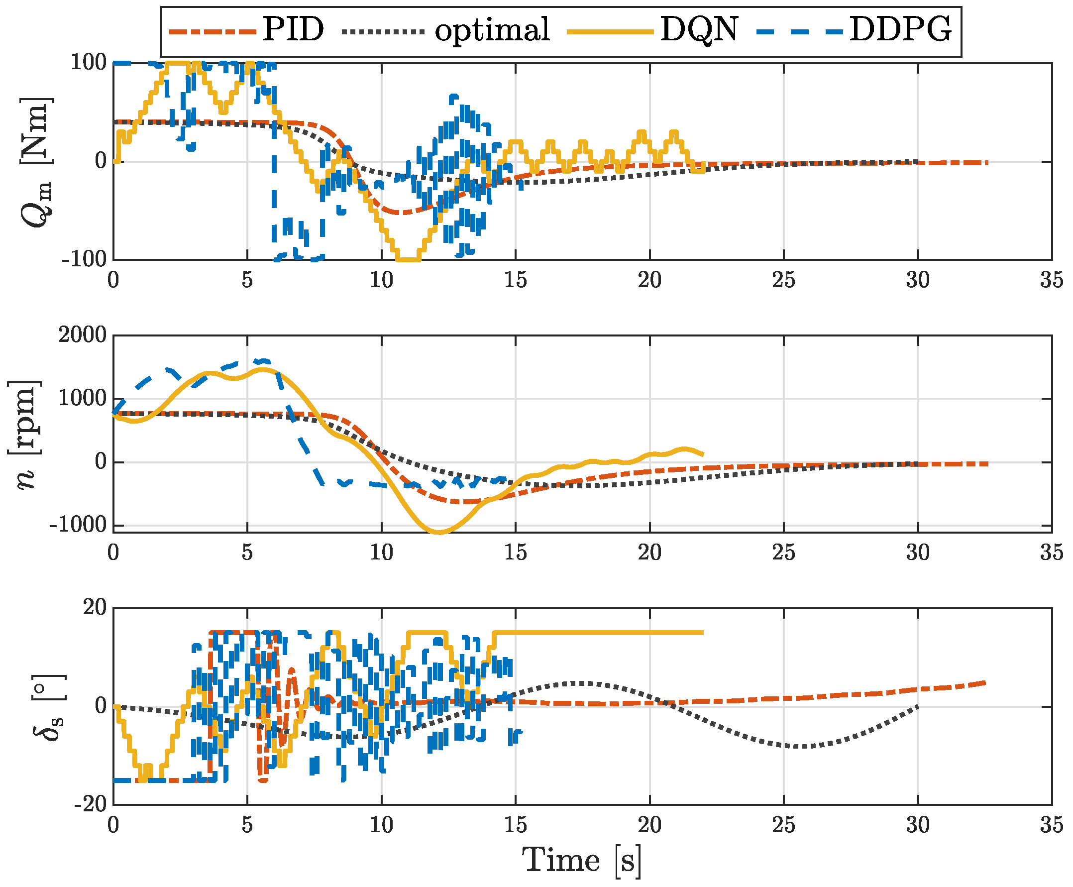
The performance of the AUV during the docking manoeuvre under the different control strategies is shown in Figure 9, Figure 10 and Figure 11. Figure 9 shows the time evolution of the translations in surge and heave and the rotation in pitch. The docking point was placed at $x=20$ m and $z=0$ m and zero pitch angle was desired. The time evolution of the translational and rotational velocities can be seen in Figure 10. The control input to the motor and sternplane is shown in Figure 11 for the different control schemes in addition to the motor rotational speed.

The DQN and DDPG curves show results after learning for 10,000 episodes. During learning, the starting vertical position of the AUV was randomly initialised in the range [0.9,1.1], as recommended by Gaudet et al. [32]. However, here, the starting position was fixed at $z=1$ m.

Note that the signals had a different duration for each control algorithm, since the docking criteria (as defined by Equation (17)) were met at different times.

Table 5. Order of magnitude of the mean computational time (in seconds) required by each algorithm during training and deployment.

Algorithm	PID	Optimal Parametric	DQN	DDPG
Training (total)	-	-	${10}^5$	${10}^5$
Deployment (at every time step)	${10}^{-4}$	${10}^2$	${10}^{-3}$	${10}^{-3}$

summarises the computational time required by each control scheme during deployment and training when running on an Intel Core i7-6700 quadcore processor with 32 GB RAM with the selected MATLAB/Simulink implementation. In fact, only the order of magnitude is shown to enable a clearer comparison. Note that training is required only for the RL algorithms.

6. Discussion

As can be seen in Figure 9, the DDPG algorithm results in the shortest docking time, while PID control in the longest time. However, as shown in Figure 10, the DQN scheme is best at slowing down the AUV in the horizontal direction, whereas the DDPG control presents a high and potentially dangerous final velocity.

In Figure 11, it is clear that the PID and parametric optimal control present the smoothest control signals. In particular, the weights in Equation (21) ensure neither the torque nor the sternplane angle saturation limits are exceeded. While the DQN algorithm presents some oscillations, the control signals of the trained DDPG scheme are very noisy and present an almost bang-bang type of behaviour. This chattering behaviour is a particularly interesting feature, which is likely to be caused by the layer with the hyperbolic tangent activation function in the deep neural network of the actor in Figure 7. The bang-bang behaviour of the DDPG is unlikely to be achievable in reality due to the physical limits of the motor and sternplane. This problem could be alleviated by including the change in the value of the actions as a penalty in the cost function. However, to ensure learning, the previous action signals should also be tracked in a scheme more similar to SARSA than Q-learning [41].

In Figure 11, it is also interesting to notice that all algorithms show an initial high positive motor torque signal, followed by a dip into negative values and then a settling onto zero torque. The dip corresponds to an inversion in the thrust direction which ensures the AUV breaks before reaching the docking point, as reflected in Figure 10. An inversion in the propeller revolutions is undesirable, since in practice it could result in cavitation (depending on the depth of the AUV) and/or increased loading on the propeller blades, whose associated higher drag and turbulent flow is not described by the simple model employed here. However, inverting the direction of the thrust is fundamental to reduce the docking time, whilst ensuring a soft contact to the docking station. Although it would be possible to prioritise the avoidance of the motor breaking effect in favour of breaking purely through damping at the expense of a longer docking time, maintaining relatively high forward speed ensures the AUV has sufficient handling abilities as close to the docking station as possible. High manoeuvrability is especially desirable in situations where there are strong disturbances, e.g., due to ocean currents, or where the AUV is attempting to dock onto a moving platform, e.g., for retrieval from a floating vessel.

The better performance of DQN over DDPG is also reflected in Figure 8, with DQN exhibiting a higher mean average reward per episode. However, the standard deviation of the curves is still very high with no clear plateau as compared with [44,46,47]. Hence, it is likely that both DQN and DDPG algorithms have not fully converged yet after 10,000 episodes. For instance, Haarnoja et al. [47] showed results after 10 million steps. Therefore, further improvements over the policies shown here are possible for the DQN and DDPG schemes. Similarly, investigating different network architectures with hyper-parameter tuning can further improve the performance of both algorithms.

Overall, the DQN algorithm outperformed the DDPG scheme for the docking of the AUV onto a fixed platform in 3 DOF by presenting smoother control action signals and a lower final velocity. These features enable a realistic implementation that abides by the systems physical limits and lower the risk of damage due to high collision forces, respectively. Furthermore, DQN results in a shorter docking time as compared with PID control at the expense of an inversion in the spinning direction of the motor and propeller. The success of DQN is mainly due to the bespoke state and action signals that have been selected here, with the action space being represented by the step changes in the control input. Conversely, a bang-bang control type would be hardly achievable with real hardware. The results from the DDPG algorithm can be improved, but ultimate docking is still achieved. In the future, penalties should be imposed on changes in the motor torque and sternaplane angle. Additionally, alternative RL algorithms with continuous state and action spaces can be investigated, e.g., soft-actor critic, which present much higher performance than DDPG in complex control tasks [47].

In Table 5, it is interesting to compare the performance of RL and classical control strategies. PID control is most efficient during deployment and requires no training. However, the algorithm is more likely to suffer in more complex scenarios, e.g., under strong disturbances due to waves or currents or an AUV attempting to dock onto a moving platform. Parametric optimal control does not require training either as compared with RL strategies, which typically take up to 24 h per seed with the selected implementation on a stand-alone desktop. However, during deployment, both RL schemes are five orders of magnitude faster than parametric optimal control. In fact, optimal control would be replaced by nonlinear model predictive control with a moving window. Hence, although the computation of the control signal would be expensive for the first time step, the calculations for the subsequent time steps would take fewer resources because they can be initialised from the previous time step. Additionally, a pure C implementation is likely to be faster than the prototype code developed here. However, the point stands that RL strategies achieve comparable performance to parametric optimal control (in fact, shorter docking time), whilst presenting a much lower computational cost at deployment. Fundamentally, the computational time at deployment for both DQN and DDPG enables a realistic on-line implementation of these control schemes considering the selected time step used by the controller (0.2 s).

7. Conclusions

In this initial study, RL schemes were applied for the first time to the docking control of an AUV. In particular, classical and RL strategies were assessed for the control of an AUV attempting to dock onto a fixed platform without external disturbances. The analysis was performed in a simulation environment developed specifically for the task. The motion of the AUV was constrained to surge, heave and pitch. Benchmarking for the RL schemes was provided by PID and parametric optimal control.

Two RL algorithms were investigated: DQN and DDPG. DDPG employs continuous state and action spaces by relying on deep neural networks to approximate the state–action value (critic) and to approximate the action selection process (actor). As a result, the action signals can be selected as the control input signals, namely the motor torque and sternplane angle, while the states can be set to be the position, orientation and velocity of the AUV in addition to the propeller revolutions. Conversely, DQN presents a discrete action space and an $ϵ$-greedy policy instead of the actor. As a result, the action vector is selected as the set of positive, negative and zero step changes in the motor torque and sternplane angle, while the control input signals are added to the state space so that the absolute values can be tracked.

All algorithms successfully managed to dock the AUV onto a fixed platform. This was achieved by keeping a high speed until the AUV was close to the docking station and then breaking the vehicle’s motion by inverting the propeller revolutions so as to maintain high manoeuvrability as far as possible. While DDPG presents chattering in the control input selection due to the hyperbolic-tangent layer in the actor, the innovative DQN implementation developed here presents the best compromise between short docking time and low control effort, whilst meeting the docking objective. Evolutions of the DDPG algorithm can be used in the future to improve the performance of RL strategies with a continuous action space. Additionally, whereas parametric optimal control presents a high computational cost at deployment time, the RL schemes are much more efficient and enable an on-line implementation. Conversely, the computational burden is placed on training instead. However, this can be done through simulations and experiments. As the algorithm was implemented on the real system, the data can slowly be replaced with the data coming from the actual vehicle and the neural networks can be retrained off-line. In this way, RL can provide the performance of optimal control at a much lower computational cost at deployment. Furthermore, its model-free nature provides a general framework that can be easily adapted to the control of different systems, although it is necessary to tune the parameters for the task at hand for best results.

References

1. Allard, Y.; Shahbazian, E.; Isenor, A. Unmanned Underwater Vehicle (UUV) Information Study; Technical Report; OODA Technologies Inc.: Montreal, QC, Canada, 2014. [Google Scholar]
2. Wynn, R.B.; Huvenne, V.A.I.; Le Bas, T.P.; Murton, B.J.; Connelly, D.P.; Bett, B.J.; Ruhl, H.A.; Morris, K.J.; Peakall, J.; Parsons, D.R.; et al. Autonomous Underwater Vehicles (AUVs): Their past, present and future contributions to the advancement of marine geoscience. Mar. Geol. 2014, 352, 451–468. [Google Scholar] [CrossRef] [Green Version]
3. German, C.R.; Jakuba, M.V.; Kinsey, J.C.; Partan, J.; Suman, S.; Belani, A.; Yoerger, D.R. A long term vision for long-range ship-free deep ocean operations: Persistent presence through coordination of Autonomous Surface Vehicles and Autonomous Underwater Vehicles. In Proceedings of the IEEE/OES Autonomous Underwater Vehicles (AUV 2012), Southampton, UK, 24–27 September 2012. [Google Scholar]
4. Lane, D.M.; Maurelli, F.; Kormushev, P.; Carreras, M.; Fox, M.; Kyriakopoulos, K. Persistent autonomy: The challenges of the PANDORA project. In IFAC Proceedings Volumes (IFAC-PapersOnline); IFAC Secretariat: Laxenburg, Austria, 2012; Volume 9, pp. 268–273. [Google Scholar]
5. Griffiths, G. Technology and Applications Vehicles of Autonomous Underwater; Taylor & Francis: London, UK, 2003. [Google Scholar]
6. LiVecchi, A.; Copping, A.; Jenne, D.; Gorton, A.; Preus, R.; Gill, G.; Robichaud, R.; Green, R.; Geerlofs, S.; Gore, S.; et al. Underwater Vehicle Charging. In Powering the Blue Economy: Exploring Opportunities for Marine Renewable Energy in Martime Markets; Chapter 3; U.S. Department of Energy, Office of Energy Efficiency and Renewable Energy: Washington, DC, USA, 2019; pp. 22–37. [Google Scholar]
7. Stokey, R.; Purcell, M.; Forrester, N.; Austin, T.; Goldsborough, R.; Allen, B.; Alt, C.V. A docking system for REMUS, an autonomous underwater vehicle. In Proceedings of the MTS/IEEE Conference Proceedings Oceans ’97, Halifax, NS, Canada, 6–9 October 1997; pp. 1132–1136. [Google Scholar]
8. Mcewen, R.S.; Hobson, B.W.; Bellingham, J.G. Docking Control System for a 21 in Diameter Auv. IEEE J. Ocean. Eng. 2008, 33, 550–562. [Google Scholar] [CrossRef]
9. Li, D.J.; Chen, Y.H.; Shi, J.G.; Yang, C.J. Autonomous underwater vehicle docking system for cabled ocean observatory network. Ocean Eng. 2015, 109, 127–134. [Google Scholar] [CrossRef]
10. Palomeras, N.; Vallicrosa, G.; Mallios, A.; Bosch, J.; Vidal, E.; Hurtos, N.; Carreras, M.; Ridao, P. AUV homing and docking for remote operations. Ocean Eng. 2018, 154, 106–120. [Google Scholar] [CrossRef]
11. Palomeras, N.; Peñalver, A.; Massot-Campos, M.; Negre, P.L.; Fernández, J.J.; Ridao, P.; Sanz, P.J.; Oliver-Codina, G. I-AUV docking and panel intervention at sea. Sensors 2016, 16, 1673. [Google Scholar] [CrossRef] [PubMed]
12. Kimball, P.W.; Clark, E.B.; Scully, M.; Richmond, K.; Flesher, C.; Lindzey, L.E.; Harman, J.; Huffstutler, K.; Lawrence, J.; Lelievre, S.; et al. The ARTEMIS under-ice AUV docking system. J. Field Robot. 2018, 35, 299–308. [Google Scholar] [CrossRef]
13. Tan, C.S.; Sutton, R.; Ahmad, S.; Chudley, J. Autonomous underwater vehicle retrieval manoeuvre using artificial intelligent strategy. In IFAC Proceedings Volumes (IFAC-PapersOnline); IFAC Secretariat: Laxenburg, Austria, 2003; Volume 36, pp. 139–144. [Google Scholar]
14. Ahmad, S.M.; Sutton, R.; Burns, R.S. Retrieval of an Autonomous Underwater Vehicle: An Interception Approach. Underw. Technol. 2003, 25, 185–197. [Google Scholar] [CrossRef]
15. Hardy, T.; Barlow, G. Paper on UUV Deployment and Retrieval Options for Submarines presented at INEC; INEC: Abuja, Nigeria, 2008. [Google Scholar]
16. Sarda, E.I.; Dhanak, M.R. Launch and Recovery of an Autonomous Underwater Vehicle From a Station-Keeping Unmanned Surface Vehicle. IEEE J. Ocean. Eng. 2019, 44, 290–299. [Google Scholar] [CrossRef]
17. Jantapremjit, P.; Wilson, P.A. Control and Guidance Approa ch Using an Autonomous Underwater Vehicle. Int. J. Marit. Eng. Sci. 2008, 150, 1–12. [Google Scholar]
18. Yan, Z.; Xu, D.; Chen, T.; Zhou, J.; Wei, S.; Wang, Y. Modeling, Strategy and Control of UUV for Autonomous Underwater Docking Recovery to Moving Platform. In Proceedings of the 36th Chinese Control Conference, Dalian, China, 26–28 July 2017. [Google Scholar]
19. Li, Y.; Jiang, Y.; Cao, J.; Wang, B.; Li, Y. AUV docking experiments based on vision positioning using two cameras. Ocean Eng. 2015, 110, 163–173. [Google Scholar] [CrossRef]
20. Sans-Muntadas, A.; Brekke, E.F.; Hegrenæs, Ø.; Pettersen, K.Y. Navigation and probability assessment for successful AUV docking using USBL. IFAC-PapersOnLine 2015, 28, 204–209. [Google Scholar] [CrossRef]
21. Vallicrosa, G.; Ridao, P. Sum of gaussian single beacon range-only localization for AUV homing. Ann. Rev. Control 2016, 42, 177–187. [Google Scholar] [CrossRef]
22. Myint, M.; Yonemori, K.; Lwin, K.N.; Yanou, A.; Minami, M. Dual-eyes Vision-based Docking System for Autonomous Underwater Vehicle: An Approach and Experiments. J. Intell. Robot. Syst. Theory Appl. 2017, 92, 1–28. [Google Scholar] [CrossRef]
23. Sans-Muntadas, A.; Pettersen, K.Y.; Brekke, E.; Kelasidi, E. Learning an AUV docking maneuver with a convolutional neural network. Proc. IEEE Oceans 2017, 8, 100049. [Google Scholar] [CrossRef]
24. Hall, R.; Anstee, S. Trim Calculation Methods for a Dynamical Model of the REMUS 100 Autonomous Underwater Vehicle; Technical Report; DSTO: Canberra, Australia, 2011.
25. Jewison, C.M. Guidance and Control for Multi-Stage Rendezvous and Docking Operations in the Presence of Uncertainty. Ph.D. Thesis, Massachusetts Institute of Technology, Cambridge, MA, USA, 2017. [Google Scholar]
26. El-Fakdi, A.; Carreras, M.; Palomeras, N.; Ridao, P. Autonomous Underwater Vehicle Control Using Reinforcement Learning Policy Search Methods. In Proceedings of the Europe OCEANS 2005, Brest, France, 20–23 June 2005. [Google Scholar]
27. Fjerdingen, S.A.; Kyrkjebø, E.; Transeth, A.A. AUV Pipeline Following using Reinforcement Learning. In Proceedings of the 41st International Symposium on Robotics, Munich, Germany, 7–9 June 2010; VDE: Munich, Germany, 2010. [Google Scholar]
28. Carlucho, I.; De Paula, M.; Wang, S.; Menna, B.V.; Petillot, Y.R.; Acosta, G.G. AUV Position Tracking Control Using End-to-End Deep Reinforcement Learning. In Proceedings of the OCEANS 2018 MTS/IEEE Charleston, Charleston, SC, USA, 22–25 October 2018. [Google Scholar]
29. Yu, R.; Shi, Z.; Huang, C.; Li, T.; Ma, Q. Deep reinforcement learning based optimal trajectory tracking control of autonomous underwater vehicle. In Proceedings of the 36th Chinese Control Conference (CCC), Dalian, China, 26–28 July 2017; pp. 4958–4965. [Google Scholar]
30. Carlucho, I.; De Paula, M.; Wang, S.; Petillot, Y.; Acosta, G.G. Adaptive low-level control of autonomous underwater vehicles using deep reinforcement learning. Robot. Auton. Syst. 2018, 107, 71–86. [Google Scholar] [CrossRef] [Green Version]
31. Wu, H.; Song, S.; You, K.; Wu, C. Depth Control of Model-Free AUVs via Reinforcement Learning. IEEE Trans. Syst. Man Cybern. Syst. 2018. [Google Scholar] [CrossRef]
32. Gaudet, B.; Linares, R.; Furfaro, R. Deep Reinforcement Learning for Six Degree-of-Freedom Planetary Powered Descent and Landing. arXiv 1810, arXiv:1810.08719v1. [Google Scholar]
33. Fossen, T.I. Handbook of Marine Craft Hydrodynamics and Motion Control, 1st ed.; John Wiley & Sons: Hoboken, NJ, USA, 2011. [Google Scholar]
34. Süli, E.; Mayers, D. An Introduction to Numerical Analysis, paperback ed.; Cambridge University Press: Cambridge, MA, USA, 2003. [Google Scholar]
35. Anderlini, E.; Parker, G.G.; Thomas, G. Control of a ROV carrying an object. Ocean Eng. 2018, 165, 307–318. [Google Scholar] [CrossRef]
36. Liberzon, D. Calculus of Variations and Optimal Control Theory: A Concise Introduction; Princeton University Press: Princeton, NJ, USA, 2012. [Google Scholar]
37. Agostini, M.J.; Parker, G.G. Command Shaping Nonlinear Inputs Using Basis Functions. J. Intell. Mater. Syst. Struct. 2002, 13, 181. [Google Scholar] [CrossRef]
38. Agostini, M.J.; Parker, G.G.; Schaub, H.; Groom, K.; Robinett, R.D. Generating swing-suppressed maneuvers for crane systems with rate saturation. IEEE Trans. Control Syst. Technol. 2003, 11, 471–481. [Google Scholar] [CrossRef]
39. Rizzo, D.M.; Parker, G.G. Determining optimal state of charge for a military vehicle microgrid. Int. J. Powertrains 2014, 3, 303. [Google Scholar] [CrossRef]
40. Yakimenko, O.A. Direct Method for Rapid Prototyping of Near-Optimal Aircraft Trajectories. J. Guid. Control Dyn. 2000, 23, 865–875. [Google Scholar] [CrossRef] [Green Version]
41. Sutton, R.S.; Barto, A.G. Reinforcement Learning, hardcover ed.; MIT Press: Cambridge, MA, USA, 1998; p. 344. [Google Scholar]
42. Francois-Lavet, V.; Henderson, P.; Islam, R.; Bellemare, M.G.; Pineau, J. An Introduction to Deep Reinforcement Learning. Found. Trends Mach. Learn. 2018, 11, 219–354. [Google Scholar] [CrossRef] [Green Version]
43. Busoniu, L.; Babuska, R.; Schutter, B.D.; Ernst, D.; Busoniu, L.; Babuska, R.; Schutter, B.D.; Ernst, D. Reinforcement Learning and Dynamic Programming Using Function Approximators, 1st ed.; CRC Press: Boca Raton, FL, USA, 2010. [Google Scholar]
44. Mnih, V.; Kavukcuoglu, K.; Silver, D.; Rusu, A.a.; Veness, J.; Bellemare, M.G.; Graves, A.; Riedmiller, M.; Fidjeland, A.K.; Ostrovski, G.; et al. Human-level control through deep reinforcement learning. Nature 2015, 518, 529–533. [Google Scholar] [CrossRef] [PubMed]
45. Lillicrap, T.P.; Hunt, J.J.; Pritzel, A.; Heess, N.; Erez, T.; Tassa, Y.; Silver, D.; Wierstra, D. Continuous control with deep reinforcement learning. In Proceedings of the International Conference on Learning Representations, San Juan, Puerto Rico, 2–4 May 2016. [Google Scholar]
46. Fujimoto, S.; van Hoof, H.; Meger, D. Addressing Function Approximation Error in Actor-Critic Methods. In Proceedings of the 35th International Conference on Machine Learning, Stockholm, Sweden, 10–15 July 2018. [Google Scholar]
47. Haarnoja, T.; Zhou, A.; Abbeel, P.; Levine, S. Soft Actor-Critic: Off-Policy Maximum Entropy Deep Reinforcement Learning with a Stochastic Actor. In Proceedings of the 35th International Conference on Machine Learning, Stockholm, Sweden, 10–15 July 2018. [Google Scholar]
48. Abbeel, P. Apprenticeship Learning and Reinforcement Learning with Application to Robotic Control. Ph.D. Thesis, Stanford University, Stanford, CA, USA, 2008. [Google Scholar]
49. Mnih, V.; Silver, D.; Riedmiller, M. Playing Atari with Deep Reinforcement Learning. In Proceedings of the NIPS Deep Learning Workshop 2013, Lake Tahoe, CA, USA, 9 December 2013; pp. 1–9. [Google Scholar]
50. Anderlini, E.; Forehand, D.I.M.; Stansell, P.; Xiao, Q.; Abusara, M. Control of a Point Absorber using Reinforcement Learning. IEEE Trans. Sustain. Energy 2016, 7, 1681–1690. [Google Scholar] [CrossRef]
51. Anderlini, E.; Forehand, D.I.; Bannon, E.; Abusara, M. Control of a Realistic Wave Energy Converter Model Using Least-Squares Policy Iteration. IEEE Trans. Sustain. Energy 2017, 8, 1618–1628. [Google Scholar] [CrossRef] [Green Version]
52. Arora, J.S. Introduction to Optimum Design, 3rd ed.; Academic Press: Cambridge, MA, USA, 2012; pp. 377–409. [Google Scholar]
53. Hutchinson, I.H. A Student’s Guide to Numerical Methods; Cambridge University Press: Cambridge, UK, 2015. [Google Scholar]
54. Kingma, D.P.; Ba, J.L. Adam: A Method for Stochastic Optimization. arXiv 2015, arXiv:1412.6980. [Google Scholar]
55. Goodfellow, I.; Bengio, Y.; Courville, A. Deep Learning; MIT Press: Cambridge, MA, USA, 2016. [Google Scholar]
Figure 1. Diagram of the docking of an AUV onto a moving platform in surge, heave and pitch.
Applsci 09 03456 g001
Figure 2. Diagram of the PID control algorithm for the docking control of an AUV.
Applsci 09 03456 g002
Figure 3. Reinforcement learning diagram.
Applsci 09 03456 g003
Figure 4. Diagram of the DQN algorithm for the docking control of an AUV.
Applsci 09 03456 g004
Figure 5. Diagram of the DDPG algorithm for the docking control of an AUV.
Applsci 09 03456 g005
Figure 6. Diagram of the neural network used to approximate the action-value function by the critic of the DQN algorithm.
Applsci 09 03456 g006
Figure 7. Diagram of the neural networks used: to approximate the action-value function by the critic (a); and to select the action that maximises the discounted reward by the actor (b) of the DDPG algorithm.
Applsci 09 03456 g007
Figure 8. Convergence of the average reward per episode with episode number for the DQN and DDPG algorithms.
Applsci 09 03456 g008
Figure 9. Translation and rotation of the AUV during docking with different control strategies.
Applsci 09 03456 g009
Figure 10. Translational and rotational velocity of the AUV during docking with different control strategies.
Applsci 09 03456 g010
Figure 11. Input motor torque, motor rotational speed and input sternplane angle of the AUV during docking with different control strategies.
Applsci 09 03456 g011