Fault Diagnosis of Rolling Bearings in Rail Train Based on Exponential Smoothing Predictive Segmentation and Improved Ensemble Learning Algorithm

Featured Application

The proposed model of this paper is for the fault diagnosis of rolling bearings in rail train.

Abstract

The rolling bearing is a key component of the bogie of the rail train. The working environment is complex, and it is easy to cause cracks and other faults. Effective rolling bearing fault diagnosis can provide an important guarantee for the safe operation of the track while improving the resource utilization of the rolling bearing and greatly reducing the cost of operation. Aiming at the problem that the characteristics of the vibration data of the rolling bearing components of the railway train and the vibration mechanism model are difficult to establish, a method for long-term faults diagnosis of the rolling bearing of rail trains based on Exponential Smoothing Predictive Segmentation and Improved Ensemble Learning Algorithm is proposed. Firstly, the sliding time window segmentation algorithm of exponential smoothing is used to segment the rolling bearing vibration data, and then the segmentation points are used to construct the localized features of the data. Finally, an Improved AdaBoost Algorithm (IAA) is proposed to enhance the anti-noise ability. IAA, Back Propagation (BP) neural network, Support Vector Machine (SVM), and AdaBoost are used to classify the same dataset, and the evaluation indexes show that the IAA has the best classification effect. The article selects the raw data of the bearing experiment platform provided by the State Key Laboratory of Rail Traffic Control and Safety of Beijing Jiaotong University and the standard dataset of the American Case Western Reserve University for the experiment. Theoretical analysis and experimental results show the effectiveness and practicability of the proposed method.

1. Introduction

In various large industrial equipment, the rolling bearing is a key equipment in the rotor system; moreover, it frequently works in the adverse environment of high velocity, high temperature, high voltage, etc., this is the very reason why it is particularly important to exercise fault diagnosis over it through its real-time monitoring data [1]. In the rail transit field, the potential fault of rolling bearing has seriously threatened the rail transit safety, especially nowadays the rapid popularization of high-speed railway puts up the urgent requirement of real-time monitoring and online fault analysis to the critical equipment of rolling bearing [2,3,4,5]. By installing sensors at the special location of rolling bearing, vibration data are obtained that possess the characteristics of large amount, nonlinear, and non-stationary [6,7]. A rapid and effective fault diagnosis algorithm is the key to the systematic implementation [8,9].

The fault diagnosis algorithms of equipment mainly include statistical-based methods, signal processing-based methods, analytical model-based methods, and knowledge-based methods [10,11]. The statistical-based method is to compare the statistical characteristics of faults and normal time-domain data. Gustafsson et al. proposed to compare the peak value of the vibration acceleration data of the bearing with the peak value of normal bearing to judge the running state of the bearing [12]. The signal processing-based methods include time-domain and frequency-domain analysis methods [13,14,15,16]. Fourier transform is one of the classical frequency-domain analysis methods. The feature extraction methods for nonlinear, non-stationary signals are mainly wavelet transform and Hilbert transform [17,18]. On this basis, researchers have proposed some new improved methods, including improved denoising method based on empirical mode decomposition and improved Hilbert Huang transform method (HHT) [19], bearing fault diagnosis method based on adaptive Fourier decomposition, fault diagnosis method based on new nonlinear dynamic model, and fusion of time-frequency-domain feature parameters. Duan et al. [20] proposed a fault diagnosis method by combining local mean decomposition (LMD) and the ratio correction method to process the short-time signals. The vibration signal of rolling bearing is decomposed into a series of product functions (PFs) by LMD. The PF, which contains the richest fault information, is selected to perform envelope spectrum analysis by the Hilbert transform (HT). Ding et al. [21] proposed a new method based on wavelet denoising and nonlinear independent component analysis (ICA) to tackle the nonlinear blind source separation problem with additive noise. The analytical model-based method includes state estimation method and parameter estimation method [22,23]. State estimation is a method of estimating the internal state of a dynamic system based on available measurement data. The use of state estimation to design a distributed fault observer can solve the problem that the calculation is difficult when there are uncertain parameters in the system. Parameter estimation is the process of calculating system model parameters using system input and output data when the system model structure is known. Commonly used methods of parameter estimation include moment estimation, least squares estimation, maximum likelihood estimation, etc. With the increasing complexity of industrial equipment systems, the number and types of data recorded during the monitoring process are increasing. Knowledge-based fault diagnosis methods have gradually become the mainstream method in the field of monitoring [24]. Among them, artificial neural network [25], D-S evidence theory [26], Bayesian [27] are the most widely used. This kind of method, which can be applied in nonlinear, dynamic, and high-latitude systems can avoid the establishment of complex mechanism models. Islam et al. [28] proposed an online fault diagnosis system for bearings that detects emerging fault modes and then updates the diagnostic system knowledge (DSK) to incorporate information about the newly detected fault modes.

Directed at the characteristics of nonlinear and non-stationary data of rail train, a complete long-term fault diagnosis method for rolling train rolling bearings based on exponential smoothing prediction and improved integrated learning algorithm is designed and applied to the measured bearing data set designed in this paper. The Sliding Window based on Exponential Smoothing Segmentation Algorithm (SWESSA) is used in this method to segment the original data. Then, the local feature extraction is performed on the segmented data, and the improved local frequency is defined. The extreme point is replaced by the segmentation point as a marker for judging the motion limit, which can eliminate the interference from high-frequency noise and multi-excitation source to local frequency. Finally, the Improved AdaBoost Algorithm (IAA) is used to classify the sample data. Before the classification, the sample data is clustered to filter the noise data, so the anti-noise ability is enhanced, and the classification effect is improved.

In this paper, the vibration data of the rolling bearing of the rail train is analyzed, and the fault is diagnosed. The content of this paper is divided into the following parts: Section 2 introduces the complete process of the proposed fault diagnosis method for the rolling bearing of the rail train and the specific work of each part. Section 3 introduces the time-series segmentation method, feature extraction algorithm based on local spectrum, and the specific algorithm flow of IAA. Section 4 presents the experimental results and analysis of the proposed method, and Section 5 concludes the paper.

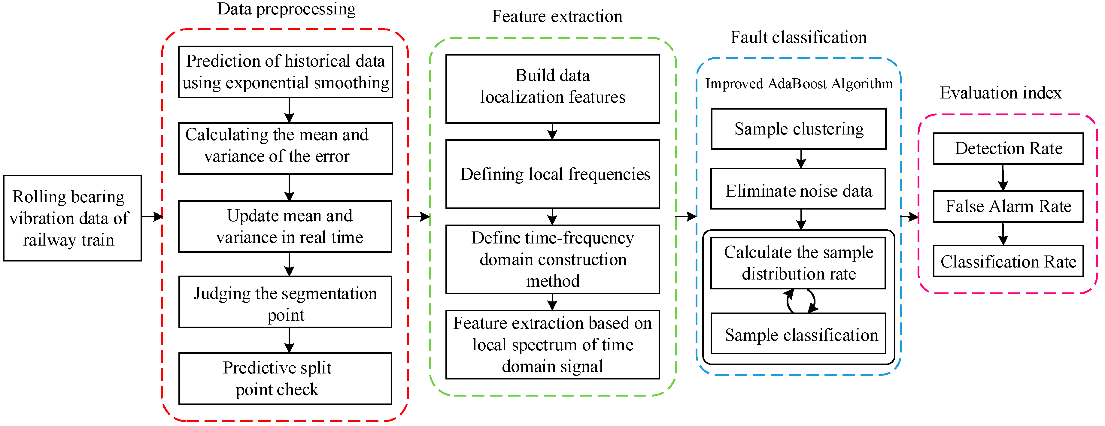
2. Complete Fault Diagnosis Process

The complete fault diagnosis process of rolling bearing mainly consists of four steps of data preprocessing, feature extraction, fault diagnosis, and evaluation index. The fault diagnosis process includes the data analysis to the diagnosis results. The classification and comparison experiments are carried out based on effective data, and the evaluation is carried out to prove the effectiveness of the method. This paper designed a way of diagnosis directed on the four major steps, respectively, as shown in Figure 1.

The specific implementation of the steps is as follows.

(1)

Firstly, the data is cleaned, and the data dimension is unified by the method of data visualization; then the exponential smoothing method is used to smooth the sequence to eliminate the random error, and the main trend of the time-series is obtained. The adaptive sliding window model based on the short-term prediction ability of the exponential smoothing method and the statistical characteristics of historical data is used to segment the time-series data, and the relationship between the statistical characteristics of the historical data and the prediction error is used to determine the segmentation point.

In the process of detecting data and transmitting data by the sensor, it is possible to be interfered to obtain an unrealized outlier point. Therefore, in the process of detecting the segmentation point, it is necessary to add a verification step to determine that the obtained split point is not an outlier generated due to interference. In the verification step, the method of setting the flag is used, that is, when a certain point of the time-series does not satisfy the historical trend, the point is set as a suspicious segmentation point. Then, check the next point, when the next point also does not satisfy the historical trend, the suspect split point is determined as the split point, and the flag bit is set; otherwise, the suspicious segmentation point is determined to be the outlier point, and the flag bit is cleared.

(2)

The nonlinear and non-stationary data characteristics extraction method based on local frequency is designed, which smartly combines the split point obtained from preprocessed data with the spectrum analysis and constructs the localization feature of data. Then, the definition of local frequency and the construction method of time-frequency-domain to proceed with the feature extraction are finalized. This method overcomes the limitation of HHT, only applicable to describe the narrowband signal, while in the meantime, it makes up the setback of Fourier global frequency, which is only worthy for unlimited fluctuating periodical signals.

(3)

Aiming at the shortcomings of the AdaBoost algorithm in anti-noise, an Improved AdaBoost Algorithm (IAA) is proposed. The method first clusters the data, filters out the noise data, and then combines AdaBoost for classification experiments which enhances the anti-noise ability and improves the classification accuracy. During the learning of the base classifier, the distribution rate of the sample is continuously calculated, and the samples with excessive sample distribution rate are deleted. The IAA is compared with the current mainstream Back Propagation (BP) neural network, standard SVM, and AdaBoost. The classification results of each classification algorithm are obtained through experiments.

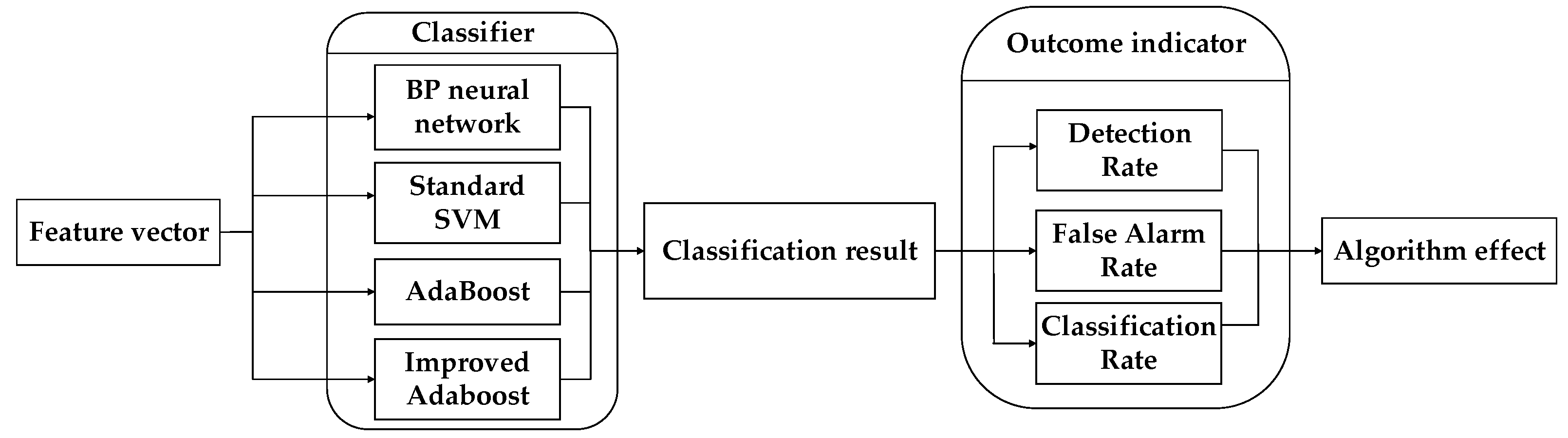
(4)

To compare the performance of each classification algorithm, three evaluation indexes, namely Detection Rate (DR), False Alarm Rate (FAR), and Classification Rate (CR), are defined. The classification results of BP neural network, standard SVM network, AdaBoost, and IAA are evaluated, respectively. The superiority of the IAA is reflected by comparison.

The whole fault diagnosis method is synthesized. From the perspective of the research object, this method comprehensively considers the characteristics of the data and the relevance and provides a reliable diagnosis strategy for the fault diagnosis of the track rolling bearing.

3. Fault Diagnosis Method

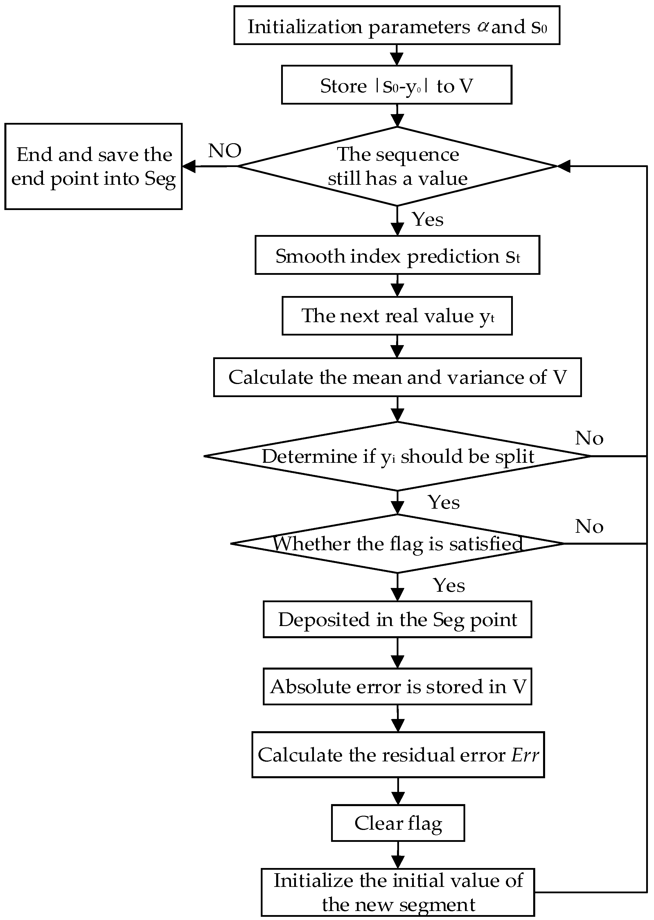
3.1. Time-Series Segmentation

Rail transit rolling bearing data is massive online data, and the overall processing is large. If the data analysis is performed directly on the original time-series, the time and space cost will be too high. In response to this situation, the original sequence is generally segmented first, and then the segmented data is subjected to feature extraction. The cost of analyzing and processing the extracted data features is much lower. We have done some work on time-series segmentation and feature extraction. The proposed SWESSA [29] can quickly and efficiently segment online data, and using local spectrum for feature extraction of rolling bearing faults [30], which can better highlight the local features of the data, clearly has strong anti-noise ability.

Time-series segmentation as an important step in time-series mining and time-series representation must meet two basic requirements: streamlining and computational efficiency. Streamlining means that the algorithm must guarantee fewer segments and smaller residual errors; computational efficiency means that the segmentation algorithm can adapt to the online computing environment [31]. For the rolling bearing data applied in this paper, it needs to have a certain anti-interference ability for data noise while being compact and computationally efficient.

For time-series segmentation, the practical meaning is time-series dimension reduction. The most important question is how to quickly and accurately detect the split point. The earliest online segmentation algorithms include the classic Sliding Window algorithm (SW), proposed by Keogh [32], and Sliding Windows and Bottom-up algorithm (SWAB) [33]. To enhance the approximation effect, we proposed a Sliding Window based on Exponential Smoothing Segmentation Algorithm (SWESSA) [29]. The basic idea is to smooth the sequence and eliminate random errors with the exponential smoothing method and then obtain the main trend of time-series. The adaptive sliding window model based on the short-term prediction ability of the exponential smoothing method and the statistical characteristics of historical data is used to segment the time-series data, obtain the data trend through prediction, and judge the segmentation point by the relationship between the statistical characteristics of the historical data and the prediction error.

We have compared the performance of SWESSA, SW, and SWAB from the normal segmentation number (NSN), normal residual error (NRES), and calculation time (NTIME) in the literature [29], as shown in

Table 1. Performance comparison of different segmentation algorithms.

Indicator	SW	SWAB	SWESSA
NSN	1	0.982	1.028
NRES	1	1.052	0.978
NTIME	1	2.372	0.852

NSN: normal segmentation number; NRES: normal residual error; NTIME: calculation time; SW: Sliding Window; SWAB: Sliding Windows and Bottom-up; SWESSA: Sliding Window based on Exponential Smoothing Segmentation Algorithm.

. The NSN for SW and SWAB and SWESSA is the same. NRES represents the error between the segmentation result and the original data. The smaller the NRES, the better the segmentation effect. The SWESSA is closer to the original sequence than SW and SWAB, and the NRES is the smallest. The NTIME only includes the time to calculate the segmentation point and the residual error. It can be seen from the NTIME that SWESSA is better than SW and SWAB. It is proved by experiments that SWESSA can meet the task of data segmentation with efficient calculation, and it has certain anti-interference ability for data noise, paving the way for the whole fault diagnosis method.

The flow chart of SWESSA is shown in Figure 2.

Where $s_t$ represents a smooth prediction value, $y_t$ represents the true value of the time-series, $s_0$ represents the initial value of the exponential segmentation algorithm, and the calculation method is as follows:

$$s_0=(y_0+y_1+y_2)/3$$

(1)

$\alpha$ is the weight of the smoothing algorithm, $\alpha =0.2$. V represents a vector that stores absolute errors, Seg represents the set of stored partition points, and Err represents the residual error between the Linear fit of the segmentation point and the original sequence. The formula for the mean $\mu$ and the variance $\sigma$ of the absolute prediction error is as follows:

$$\mu =\frac{1}{m}{\displaystyle \sum _1^m\Delta Er{r}_i},\hspace{1em}\sigma =\sqrt{\frac{1}{m}{\displaystyle \sum _{i=1}^m{(\Delta Er{r}_i-\mu )}^2}}$$

(2)

The algorithm repeats the loop until all data is processed. After initializing the parameters:

(a)

Use a single exponential smoothing method to calculate the smoothed value $s_t$ as the predicted value of the next time point t;

(b)

Obtain the true value $y_t$ of the time point t, calculate the prediction error $y_t-s_t$, and store the value in the vector V;

(c)

Calculate the mean $\mu$ and standard deviation $\sigma$ of V, and the standard deviation and mean are updated in real-time;

(d)

Determine whether the point is a split point by Equation (3). If not, continue to loop the next point; if yes, set the flag to cache the point at the same time. If the next point also satisfies the requirements of the split point, the previous point is stored in Seg, and the initial $s_0$ of the split segment is reinitialized to continue the loop.

$$P\{\mu -2x\sigma <R<\mu +2x\sigma \}\le 1-p$$

(3)

where p is the split compression ratio of the time-series (p needs to be set in advance by user, $0<p<1$), R represents a random variable.

3.2. Feature Extraction Based on Local Spectrum of Time-Domain Signal

The focus of the feature extraction of the segmented data is to maximize the difference between different categories of samples under the premise of ensuring that the loss of sample data information is minimized. The main points of data feature parameter extraction include dimensionality reduction and noise elimination. The method mainly includes time-domain feature extraction and frequency-domain feature extraction [34]. The time-domain feature extraction method mainly extracts the time-domain feature value of each sample data as the feature value of the sample and is generally based on statistics or shape. The frequency-domain feature extraction transforms the original data from the time-domain to the frequency-domain by using the Fourier transform, so that features that are difficult to find in the time-domain can be mined. The main frequency-domain feature acquisition methods are divided into two categories - one is the global frequency defined for harmonic signals from a global perspective. While another is the instantaneous frequency, which is the reciprocal of the period [35].

In the analysis of rolling bearing faults, the time-domain analysis is random, the accuracy is not high, the feature comparison is not obvious, and the ability of noise reduction is poor. The frequency-domain analysis is effective because the vibration frequency of the bearing will be different due to the existence of the fault, which will produce a clear difference in the spectrum or power spectrum. Therefore, the frequency characteristics can not only diagnose faulty bearings but also diagnose sub-health bearings. According to the concept of global frequency and instantaneous frequency mentioned above, it is found that the applicable conditions are relatively harsh. The global frequency is suitable for periodic signals with infinite smooth fluctuations, and the instantaneous frequency is suitable for narrow-bandwidth non-stationary signals. The applicable conditions of the two are not suitable for the data signals extracted by the rolling bearings of rail train and lack of universality. So, a method for extracting fault characteristics of rolling bearings based on the local spectrum is proposed [30]. This method defines the concept of local frequency of time-domain data. The original signal can be approximated as consisting of a series of V-waves containing two adjacent segmentation points and data points between them. The local period $T(t)$ of the original signal $x(t)$ can be defined by the V-wave, as follows:

$$T(t)=t_{k+1}-t_k,t_k<t<t_{k+1}$$

(4)

$T(t)$ represents the time required for the signal to complete a local vibration in the local time range. The starting position $t(k)$ is the moment of the i-th local maximum in the original signal $x(t)$, and then the local frequency $v(t)$ is defined as the reciprocal of the generalized local period $T(t)$, namely:

$$v(t)=\frac{1}{T(t)}=\frac{1}{t_{k+1}-t_k},t_k<t<t_{k+1}$$

(5)

The local frequency $v(t)$ indicates the number of vibrations completed in the unit local time, and $v(t)$ is used to measure the speed of local vibration in Hz.

Besides, the local frequency spectrum is constructed by using the idea of constructing the frequency-domain in the global frequency spectrum, which is used to analyze the rolling bearing data. The construction method of local spectrogram and time-frequency-domain construction method are used to extract the local features of the original signal, and the segmentation points obtained by the denoising process with spectrum analysis are ingeniously combined. A set of feature extraction methods based on the local spectrum is constructed, which provides a very reliable feature vector for subsequent fault classification of rolling bearings. The physical meaning of this method, which can better highlight the local features of the data, is clearer and has strong anti-noise ability. It compensates for the shortcomings of global frequency and instantaneous frequency and optimizes the concept of the local spectrum. The author has expounded the specific process of feature extraction of the local spectrum of the time-domain signal in the literature [30].

3.3. Improved AdaBoost Algorithm

For the bearing fault diagnosis data type, the classification accuracy of general machine learning algorithms, such as BP neural network and standard SVM, can’t achieve the desired effect. However, integrated learning algorithms, such as Bagging or Boosting, can effectively improve the classification accuracy of weak classifiers. AdaBoost is a classic iterative integration algorithm in the integrated learning algorithm. It improves classification accuracy by integrating weak classifiers with weak classification. The weak classifier can be any classifier, such as a simple decision tree, a simple linear logistic classifier, a BP algorithm, and so on.

The core idea of AdaBoost is to iteratively train the weak learning algorithm for the same data set and integrate them into a strong learning algorithm. The upper limit of the training error decreases with the number of iterations, so there is no over-fitting phenomenon [36]. The strong learning algorithm can greatly improve the accuracy of the weak classifier, which is easy to encode and does not require parameter adjustment with a lower generalized bit error rate, and, at the same time, it is sensitive to outliers or noise [37]. Therefore, the initial condition is to ensure that the classifier uses the sample set data with the least noise. When there are abnormal points or noise in the data, the AdaBoost algorithm does not process it, which will seriously affect the classification result. To enhance the anti-noise ability, this paper improves the AdaBoost algorithm and proposes an improved AdaBoost algorithm (Improved AdaBoost Algorithm, IAA). The main idea of the algorithm is to filter the sample data and eliminate samples with too large sample distribution during the iterative process first, which ensure the diversity of the sample. Then, the data after denoising are classified, during which the classification accuracy is greatly improved.

First, for the noisy data, IAA first clusters the sample data to make the sample data of the same category more compact, and the difference between the different categories of sample data is greater through clustering. There are many clustering algorithms, such as Self-organizing Maps and K-means. In this paper, the improved K-means is selected to optimize the clustering process of the K-means clustering algorithm. The improved K-means eliminate the impact of random initial cluster centers on classification results and improve the discrimination of different categories. The specific optimization details of the clustering process are as follows (Take two categories as an example):

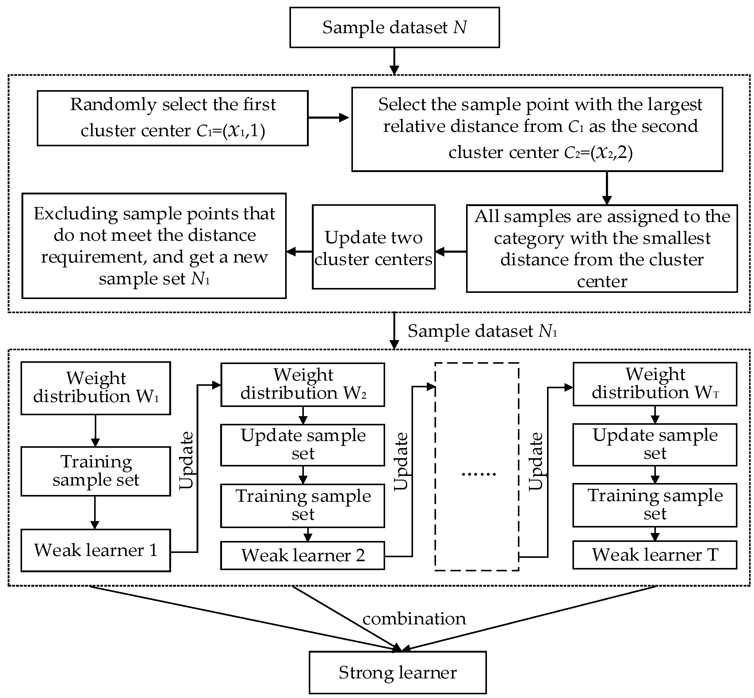
(1)

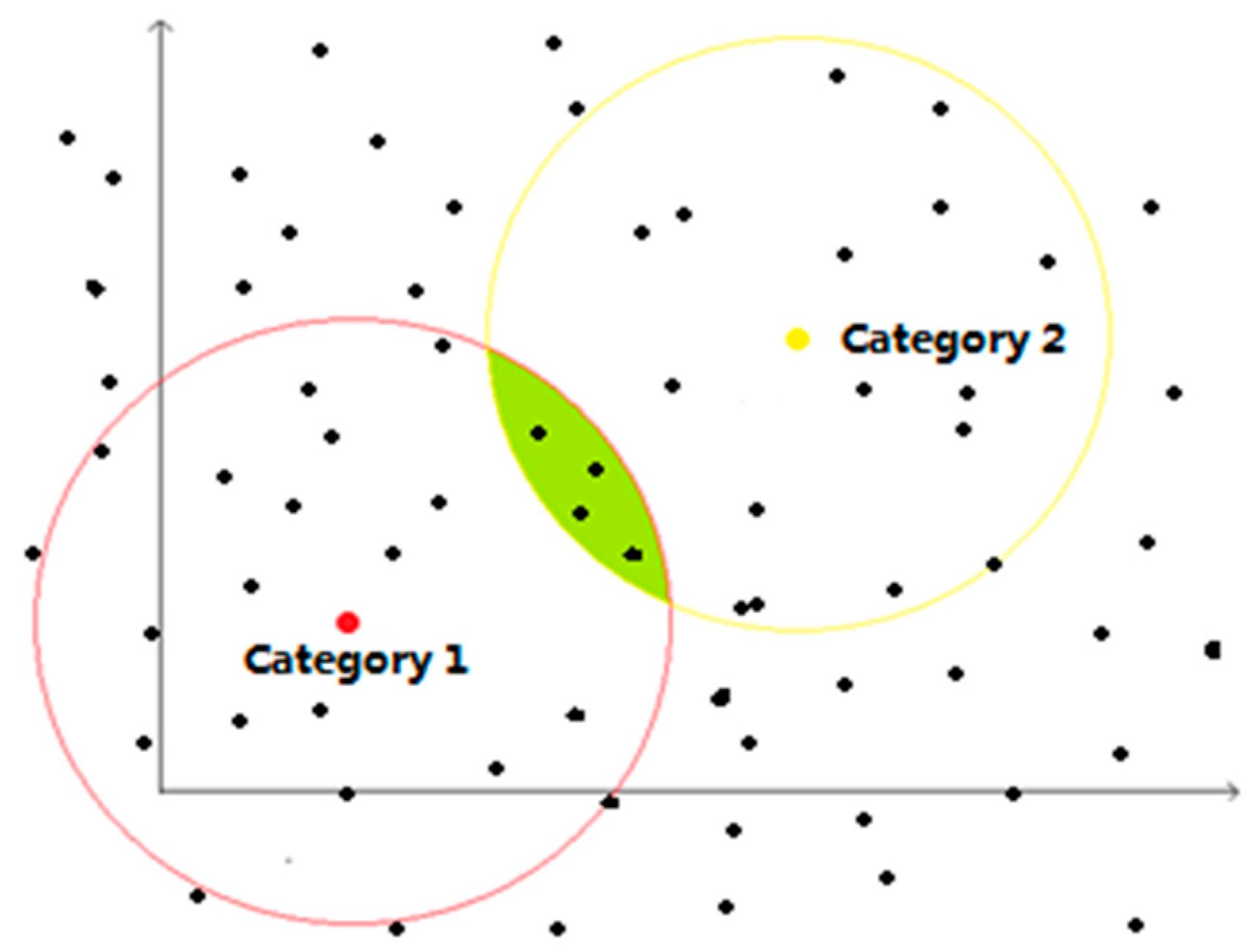
For a given sample data set, $N$ = {$(x_1,y_1)$$(x_2,y_2)$, …, $(x_n,y_n)$}, $x_i\in X$, $y_i\in Y=\{1,2\}$, where $x_i$ is the sample data with attributes of r dimensions, $y_i$ is the category to which the sample belongs. The K-means clustering operation is performed on the two types of samples, and the selection of the initial cluster center is optimized. Finally, the cluster center of the two types of samples, $({\tilde{x}}_1,1)$ and $({\tilde{x}}_2,2)$, is obtained.

(2)

Traversing all the samples in the sample dataset. All the samples belonging to category “1” are required to have a distance to ${\tilde{x}}_1$ less than $l_1$, and the distance to ${\tilde{x}}_2$ greater than $l_2$. At the same time, all the samples belonging to category “2” are required to have a distance to ${\tilde{x}}_2$ less than $l_2$, and the distance to ${\tilde{x}}_1$ greater than $l_1$. Samples that do not meet the requirements are rejected. Then, the new training set is $N_1$ = {$(x_1,y_1)$$(x_2,y_2)$, …, $(x_m,y_m)$}, $x_i\in X$, $y_i\in Y=\{1,2\}$, and Figure 3 shows the case when the number of clusters is 2 and 2 dimensions in the sample.

It is seen from the bipartite classification graph in Figure 3 that the cluster center of category ″1″ is red sample point, whereas that for category ″2″ is yellow. The red and yellow circles represent, respectively, $l_1$, $l_2$ in the above-described algorithm, i.e., at the farthest distance to the sample set center, the sample point inside the circle is the sample set of this variety while that outside the circle shall be eliminated. The green area is the common share field of the two varieties. According to the original cluster algorithm flow, the sample close to the sample center belongs to that category. To enlarge the differentiation between sample sets, the sample in the green area is to be dropped out. As a result, the two varieties of sample set become more compact, and the differences between the two are more obvious.

Second is the problem of excessive sample distribution probability. If a sample is misclassified multiple times, the distribution rate of the sample will be too large, which will interfere with the diversity of the sample data. Therefore, IAA removes samples with a distribution rate greater than $F$($F$ need to be set in advance) from the training set and distributes the distribution rate equally among the remaining samples during the iterative process of the algorithm.

Based on this optimization, IAA combines the idea of AdaBoost to learn a series of weak classifiers or weak learners and combines these weak classifiers into one strong classifier, which will improve the classification accuracy greatly. The specific block diagram of the algorithm is shown in Figure 4 (Take two categories as an example).

After the above analysis, the clustering process, the calculated sample distribution rate, and the AdaBoost algorithm are integrated. The execution steps of the complete IAA fault classification method are shown in Algorithm 1.

Algorithm 1. Execution steps of the complete IAA (Improved AdaBoost Algorithm) fault classification method.
Step	Execution Steps
Input:	Sample set $N$ = {$(x_1,y_1)$ $(x_2,y_2)$, …, $(x_n,y_n)$}, $x_i\in X$, $y_i\in Y=\{1,2,\dots ,K\}$; Number of cluster categories K; Distance parameter $l_1$, $l_2$, …, $l_K$; Maximum sample distribution rate F; Number of weak learners T; Base learning algorithm $\wp$; sum = 0.
Output:	Classification result
1:	Randomly select a point from the sample set as the cluster center $c_1=({\tilde{x}}_1,1)$
2:	fori = 1 to n
3:	Calculate the shortest Euclidean distance $d_i$ between the sample point $x_i$ and the current existing cluster center
4:	sum$\leftarrow$sum + ${d_i}^2$, $i\leftarrow i+1$
5:	end for
6:	fori = 1 to n
7:	Calculate the probability $p_i=d_i^2/sum$ that $x_i$ is selected as the next cluster center
8:	Calculate the probability interval of $x_i$
9:	end for
10:	Generate random numbers “r” between 0 and 1
11:	The sample corresponding to the interval, to which the random number “r” belongs, is the second cluster center $c_2=({\tilde{x}}_2,2)$
12:	Repeat steps 2~12 to find the third and fourth cluster centers $c_3=({\tilde{x}}_3,3)$~$c_K=({\tilde{x}}_K,K)$
13:	fori = 1 to n
14:	Calculate the Euclidean distance from $x_i$ for all cluster centers separately and classify $x_i$ into the category corresponding to the cluster center with the smallest distance
15:	Update cluster center $c_k\leftarrow \frac{1}{\left|c_k\right|}{\displaystyle \sum _{x\in c_k}x},k=1,2,\dots ,K$
16:	end for
17:	Samples in the k-th category with a distance greater than $l_k$ from $c_k$ are excluded, samples with a distance less than $l_k$ from $c_k$ and, at the same time, the distance less than $l_k$ from one of $c_1$,$c_2$,…,$c_{k-1}$,$c_{k+1}$,…,$c_K$ are excluded, get a new sample set N1
18:	fork = 1 to T
19:	Calculate the initial weight distribution $W_1=(w_{11},w_{12},\dots ,w_{1m}),w_{1i}=1/m,i=1,2,\dots ,m$ of the sample set N1
20:	Use Wk training sample set to get the k-th weak learner $G_k(x)$
21:	Calculate the classification error rate $e_k$ of $G_k(x)$ on the sample set N1
22:	Calculate the weight coefficient ${\alpha }_k$ of $G_k(x)$
23:	Update the weight distribution Wk+1 of sample set N1
24:	Update the sample distribution rate q, eliminate the sample with a sample distribution rate greater than F, update the sample set N1, and count the number of samples n
25:	Strong learner $f(x)\leftarrow f(x)+{\alpha }_k{G}_k(x)$
26:	Calculate sample classification results $G(x)=sign(f(x))$
27:	end for

4. Experimental Results and Analysis

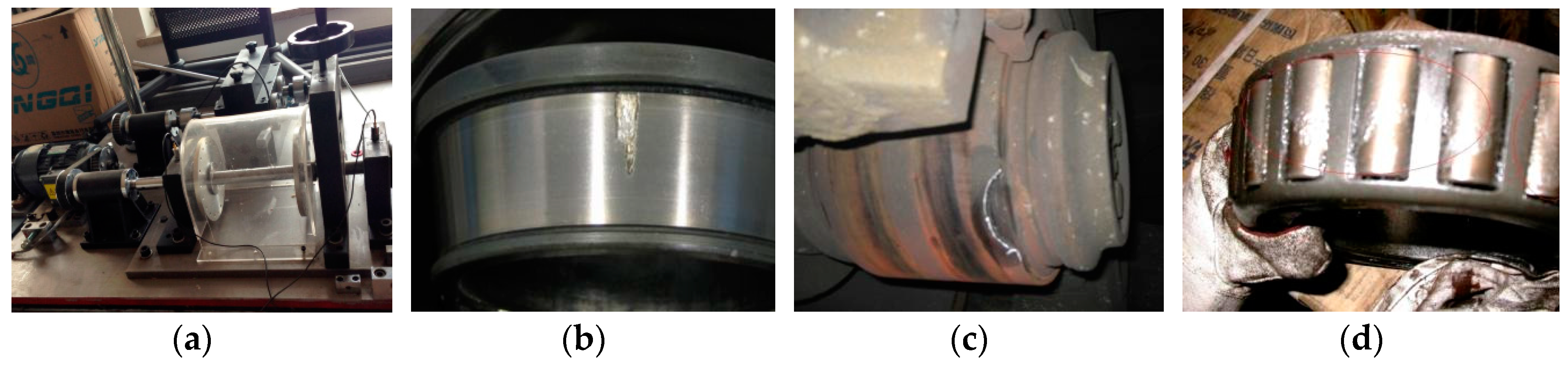
4.1. Experimental Data

The applied sample sets are the original data of rolling bearing experiment platform provided by the National Key Laboratory of Rail Transit Control and Safety under the Beijing Transport University. The main equipment used to collect the simulation data includes rolling bearing fault detection test bench, piezoelectric acceleration sensor, pulsator, data acquisition card, three types of fault rolling bearings, and normal Rolling bearings, as well as service terminals for diagnosing the collected raw data, the specific equipment, and the typical failure of train rolling bearings, as shown in Figure 5. The performance evaluation program is implemented using MATLAB. The experimental system is window10, and the experimental hardware configuration is: CPU: Intel(R) Xeon(R) CPU E5-2643, RAN size: 64 G, memory size: 12 GB × 2.

To be exact, they are the vibration data at rotating speed of 2 Hz, 4 Hz, 6 Hz, 8 Hz of the bogie rolling bearing in the running department of the rail train at normal, inner fault, outer fault, and rolling fault, respectively, and the sampling frequency is 51,200 Hz, the value is vibration acceleration, the unit is m/s². The number of samples for various sample set is 80. To increase the reliability of the experiment, the rolling bearing standard data set of the Western Reserve University is increased. The standard data set is Fan End (FE) accelerometer data and the sampling frequency is 12 kHz. The damage of the bearing is a single point of damage by electric discharge machining (EDM), and the diameter of the damage is 0.1778 mm. The data set has a rotating speed of 1796r/min, which is equivalent to 30 Hz, and the motor load is 0 hp. The following

Table 2. The sample-set information on rail transit experimental data.

Rolling Velocity	Category	Sampling Frequency	Number of Data Samples
2 Hz	Normal	51,200 Hz	80
	Inner fault	51,200 Hz	80
	Outer fault	51,200 Hz	80
	Rolling fault	51,200 Hz	80
4 Hz	Normal	51,200 Hz	80
	Inner fault	51,200 Hz	80
	Outer fault	51,200 Hz	80
	Rolling fault	51,200 Hz	80
6 Hz	Normal	51,200 Hz	80
	Inner fault	51,200 Hz	80
	Outer fault	51,200 Hz	80
	Rolling fault	51,200 Hz	80
8 Hz	Normal	51,200 Hz	80
	Inner fault	51,200 Hz	80
	Outer fault	51,200 Hz	80
	Rolling fault	51,200 Hz	80

and

Table 3. The sample-set information of standard data set.

Rolling Velocity	Category	Sampling Frequency	Number of Data Samples
30 Hz	Normal	12,000 Hz	80
	Inner fault	12,000 Hz	80
	Outer fault	12,000 Hz	80
	Rolling fault	12,000 Hz	80

show the specific detailed information of experimental data.

The normal rolling bearing time-domain diagram and fault rolling bearing timing diagram are shown in Figure 6a,b. The amplitude of the vibration acceleration of the normal bearing, which has periodicity, fluctuates around the zero points. The upper and lower fluctuation range of the amplitude is small. Also, the amplitude has Root Mean Square (RMS), Kurtosis, and Energy characteristics. The RMS is the root mean square value of the vibration amplitude. The Kurtosis is the fourth-order central moment of normalized original data, which can effectively reflect the distribution characteristics of the vibration signal. When the amplitude vibration law changes due to a malfunction or other reasons, the value of this statistic is higher than the normal value. The Energy is the sum of the squares of the amplitudes of the data signals. After a component fails, it often causes an increase in the amplitude of the vibration, increasing the amount of energy obtained. Therefore, we can see from Figure 6 that the RMS, Kurtosis, and Energy of the amplitude of the normal bearing are smaller than that of the faulty bearing.

The normal bearing time-domain diagram and fault bearing timing diagram of the sample of the standard data set are shown in Figure 7.

Each type of sample, $x_i,i=1,2,\dots ,80$ (80 is the number of samples), is converted to obtain the local frequency $v_{ij}$ of all samples. $i=1,2,\dots ,80,j=0,1,\dots ,m$, i represents the i-th sample, $v_{ij}$ represents the j-th local frequency of the i-th sample, and m is the number of intervals of the local spectrum. Then, find the maximum value Max ($v_{ij}$) and the minimum value Min ($v_{ij}$) of the local frequency in the sample, and use Max ($v_{ij}$) and Min ($v_{ij}$) as the span of all local frequency. Therefore, the interval of the local frequency of each sample is obtained as follows:

$$\frac{j}{m}[Max(v_{ij})-Min(v_{ij})]+Min(v_{ij}),i=1,2,\dots ,80,\hspace{1em}j=0,1,\dots ,m-1$$

(6)

The center frequency of the frequency interval of the top, having the highest local spectrum amplitude in the local spectrum of each sample, is extracted as the feature vectors of the sample, and the conversion of the sample data to the corresponding feature vectors is completed.

Table 4. The top five center frequency for the standard data set.

Serial Number	Normal	Inner Fault	Outer Fault	Rolling Fault
1	1202	2523	4822	3104
2	1183	2558.5	4790	3085.5
3	1267.5	2570	4831	3091
4	1256	2585	4764	3169
5	1162.5	2506	4814.5	3064

shows the top five center frequency data for the four types of samples in the standard data set. The frequency of the normal rolling bearing is mainly around 1200 Hz. The frequency of the inner fault mainly surrounds between 2500–2600 Hz. The frequency of the outer fault is mainly around 4800 Hz, and the frequency of the rolling fault is mainly concentrated at 3100 Hz. The distinction between the categories is obvious.

The specific feature vectors of the rail train experimental data set with a rotational speed of 4 Hz and standard data set are, respectively, shown in

Table 5. The feature vector of rail train experimental data.

Fault Type	Feature Vector Dimension	Feature Vector Label
4 r/s Normal	80 × 100	0
4 r/s Inner fault	80 × 100	1
4 r/s Outer fault	80 × 100	2
4 r/s Rolling fault	80 × 100	3

and

Table 6. The feature vector of standard data set.

Fault Type	Feature Vector Dimension	Feature Vector Label
Normal	80 × 100	0
Inner fault	80 × 100	1
Outer fault	80 × 100	2
Rolling fault	80 × 100	3

. As seen from the two tables, the feature vectors dimension of each sample is 100. That is, the conversion of the sample with the local spectrum and the center frequency of the top 100 frequency interval with the highest amplitude in the local spectrum are obtained as the eigenvector of the sample, and the number of samples per category is 80. The experiment classifies all the samples’ feature vectors into four categories. The effectiveness and practicability of the algorithm are determined by the evaluation indexes given in Section 4.2.

4.2. Experimental Target

Aiming to reflect the performance of the classification algorithm in an all-sided way, three evaluation indexes have been adopted in this paper. These are detection rate (DR), false alarm rate (FAR), and classification rate (CR), respectively. Their definitions are given here:

(1)  Detection Rate (DR)

DR is applied to measure the classification accuracy of a certain variety of sample set, reflecting the percentage of detected number occupying the total number of a sample set of this variety. It is shown as follows:

$$DR=\frac{\mathrm{Detected} \mathrm{number} \mathrm{of} \mathrm{sample} \mathrm{set} \mathrm{of} \mathrm{a} \mathrm{variety}}{\mathrm{total} \mathrm{number} \mathrm{of} \mathrm{sample} \mathrm{set} \mathrm{of} \mathrm{the} \mathrm{variety}}$$

(7)

(2)  False Alarm Rate (FAR)

FAR is for measuring the false alarm rate of a variety of sample set. This index is used to reflect the percentage of not belong to this variety being detected as the variety occupying the total not belong to this variety. It is shown as follows:

$$FAR=\frac{\mathrm{Number} \mathrm{of} \mathrm{data} \mathrm{not} \mathrm{belong} \mathrm{to} \mathrm{the} \mathrm{variety} \mathrm{but} \mathrm{detected} \mathrm{as} \mathrm{they} \mathrm{are}}{\mathrm{Number} \mathrm{of} \mathrm{real} \mathrm{not} \mathrm{belong} \mathrm{to} \mathrm{this} \mathrm{variety} \mathrm{data}}$$

(8)

(3)  Classification Rate (CR)

CR is applied to measure the classification accuracy for all sample set. This norm reflects the percentage of all accurately classified sample set number occupying total sample set number. The calculation is done as follows:

$$CR=\frac{\mathrm{All} \mathrm{accurately} \mathrm{classified} \mathrm{sample} \mathrm{set} \mathrm{number}}{\mathrm{Total} \mathrm{number} \mathrm{of} \mathrm{sample} \mathrm{set}}$$

(9)

In the above listed three indexes, DR and FAR reflect the probability that a certain sample set is correctly or wrongly classified, and it is directed to a single sample set. While CR reflects the entire classification effects of the algorithm. Directed to a certain variety of sample set, if DR is approaching one and FAR is approaching to 0, it means the variety of sample set is classified by higher accuracy. In the case of the entire sample set, if CR is approaching one, it indicates the entire accuracy of the classification algorithm is still higher.

4.3. Result and Analysis of Experiment

The comparison of the classification algorithm in the experiment is the BP neural network, SVM classifier, AdaBoost, and IAA. The same experimental data set is used for the comparison experiments.

Due to the stochastic character of the BP neural network, the 8 folds cross method has been adopted to conduct cross verification in this paper for the BP, i.e., the experimental data set is divided into eight equal parts, then turn is taken to have one part as the test data, while the rest seven parts as training data. This procedure is repeated eight times. Finally, the mean value of the results of each index is taken.

The standard SVM classifier is applied. Radial Basis Function (RBF) core is taken for core function, where penalty factor parameter c and RBF core function parameter g are extracted with the grid method. In the specific experimental method, $c=2^{-5},2^{-4},2^5, g=2^{-5},2^{-4},2^5$. conduct cross-verification within the scope. On completion of ergodic, the optimum values of c and g are found. If there are existing several groups of c and g, then the smallest c group is chosen. The reasons are that too high penalty factor would increase the cross-verified data accuracy rate, but possibly make the whole classifier dropped in over learning state that would lead the classifiers inferior.

AdaBoost and the IAA’s weak classifier are all applied in the BP neural network, and the number of weak classifiers is 10.

The input vector of each classifier is the feature vector of the training sample, and the results of the classification experiment are compared by the evaluation index mentioned above. The specific experimental flow is shown in Figure 8.

Classification and comparison experiments are conducted according to the experimental flow chart. The results of each algorithm based on the vibration data set at 4 r/s and the standard data set are taken as an example.

Table 7. DR (Detection Rate) performance of different algorithms.

Fault Type	BP	SVM	AdaBoost	IAA
4 r/s Inner fault	0.85	0.76	0.81	0.83
4 r/s Outer fault	0.72	0.88	0.92	0.93
4 r/s Rolling fault	0.73	0.76	0.8	0.95
Standard inner fault	0.81	0.82	0.89	0.85
Standard outer fault	0.76	0.81	0.81	0.88
Standard rolling fault	0.80	0.90	0.92	0.95
Mean	0.78	0.82	0.86	0.90

BP: Back Propagation; SVM: Support Vector Machine; IAA: Improved AdaBoost Algorithm.

shows the performance of the DR;

Table 8. FAR (False Alarm Rate) performance of different algorithms.

Fault Type	BP	SVM	AdaBoost	IAA
4 r/s Inner fault	0.03	0.07	0.07	0.03
4 r/s Outer fault	0.04	0.03	0.03	0.04
4 r/s Rolling fault	0.03	0.05	0.04	0.03
Standard inner fault	0.09	0.06	0.06	0.05
Standard outer fault	0.10	0.05	0.04	0.03
Standard rolling fault	0.07	0.06	0.05	0.05
Mean	0.060	0.053	0.048	0.038

BP: Back Propagation; SVM: Support Vector Machine; IAA: Improved AdaBoost Algorithm.

shows the performance of the FAR, and

Table 9. CR (Classification Rate) performance of different algorithms.

Fault Type	BP	SVM	AdaBoost	IAA
4r/s Inner fault	0.83	0.76	0.78	0.83
4r/s Outer fault	0.8	0.91	0.92	0.95
4r/s Rolling fault	0.73	0.76	0.81	0.9
Standard inner fault	0.70	0.85	0.90	0.91
Standard outer fault	0.84	0.83	0.83	0.88
Standard rolling fault	0.85	0.88	0.91	0.94
Mean	0.79	0.83	0.86	0.90

BP: Back Propagation; SVM: Support Vector Machine; IAA: Improved AdaBoost Algorithm.

shows the performance of the CR.

Table 7 shows that in the entire manifestation, the IAA is slightly higher than the rest few algorithms, the next is AdaBoost, then is the SVM, the last one is the BP algorithm. Each algorithm in a single data set manifests differently. In the inner fault detection rate at rotation velocity 4 r/s of the rolling bearing in the running department of rail train, the detection rate of the BP algorithm is better than the other algorithms. This means a different classification algorithm should be tried in the different data set. The good average performance does not necessarily confirm all data set. The solution is to be taken according to the specific situation.

It can be seen from Table 8 that the FAR of BP is the highest, the FAR of IAA is the lowest, and the FAR of the SVM algorithm is slightly higher than AdaBoost. This proves the shortcomings of the BP algorithm, that is, it is easily dropped in local optimum, to obtain the most satisfactory result.

It is found out from Table 9 that the overall performance on the correct rate of IAA is higher than other algorithms, approving the effectiveness of this algorithm. The next is AdaBoost, and the little inferior is the SVM algorithm. The essential cause of their similar accuracy is that AdaBoost is upgrading to weak classifier algorithm, while SVM emphasizes on largely bipartite classification. Therefore, the two algorithm effects are higher than BP neural network. BP neural network is like AdaBoost’s weak classifier, whose classification result is not satisfactorily obtained, depending on its network framework.

It can be summed up from the above three tables that the mean performance of the IAA is somewhat being raised, no matter from DR, FAR, or CR. What’s more, the 90% CR verifies that the IAA is reliably superior than the other three comparative algorithms. Simultaneously, it is testified that the algorithm is applicable in the present study and provides a reliable method for fault diagnosis of the rolling bearing in the running department of a rail train.

5. Conclusions

Through the acquisition of vibration data of rolling train rolling bearings, the bearing fault can be predicted, which can ensure driving safety and reduce operating costs. However, rolling bearing vibration data has the characteristics of a large amount of data, nonlinearity, non-stationary, etc. Therefore, directed at the characteristics of nonlinear and non-stationary data of rail train, a complete long-term fault diagnosis method for rolling train rolling bearings based on exponential smoothing prediction and improved integrated learning algorithm is designed and applied to the measured bearing data set designed in this paper. First, the data is segmented using SWESSA, then the features through the local spectrum are extracted, and the segmentation points with spectrum analysis are combined. To enhance the anti-noise ability, the AdaBoost algorithm is improved into Imported AdaBoost Algorithm. The experimental results prove the reliability and practicability of Imported AdaBoost Algorithm. The paper provides a complete set of a new method for complicated fault diagnosis on rolling bearing in a rail train, that has extremely high practical value in rolling bearing fault diagnosis.

References

- Smith, W.A.; Randall, R.B. Rolling element diagnostics using the Case Western Reserve University data: A benchmark study. Mech. Syst. Signal Process. 2015, 64–65, 100–131. [Google Scholar] [CrossRef]
- Liu, R.; Yang, B.; Zio, E.; Chen, X. Artificial intelligence for fault diagnosis of rotating machinery: A review. Mech. Syst. Signal Process. 2018, 108, 33–47. [Google Scholar] [CrossRef]
- Glowacz, A.; Glowacz, W.; Glowacz, Z.; Kozik, J. Early fault diagnosis of bearing and stator faults of the single-phase induction motor using acoustic signals. Measurement 2018, 113, 1–9. [Google Scholar] [CrossRef]
- Duan, Z.; Wu, T.; Guo, S.; Shao, T.; Malekian, R.; Li, Z. Development and trend of condition monitoring and fault diagnosis of multi-sensors information fusion for rolling bearings: A review. Int. J. Adv. Manuf. Technol. 2018, 96, 803–819. [Google Scholar] [CrossRef]
- Li, Z.; Jiang, Y.; Hu, C.; Peng, Z. Recent progress on decoupling diagnosis of hybrid failures in gear transmission systems using vibration sensor signal: A. review. Measurement 2016, 90, 4–19. [Google Scholar] [CrossRef]
- Wang, L.; Liu, Z.; Miao, Q.; Zhang, X. Time–frequency analysis based on ensemble local mean decomposition and fast kurtogram for rotating machinery fault diagnosis. Mech. Syst. Signal Process. 2018, 103, 60–75. [Google Scholar] [CrossRef]
- Zheng, K.; Luo, J.; Zhang, Y.; Li, T.; Wen, J.; Xiao, H. Incipient fault detection of rolling bearing using maximum autocorrelation impulse harmonic to noise deconvolution and parameter optimized fast EEMD. ISA Trans. 2019, 89, 256–271. [Google Scholar] [CrossRef] [PubMed]
- Lu, S.; He, Q.; Zhao, J. Bearing fault diagnosis of a permanent magnet synchronous motor via a fast and online order analysis method in an embedded system. Mech. Syst. Signal Process. 2018, 113, 36–49. [Google Scholar] [CrossRef]
- Peng, K.; Ma, L.; Zhang, K. Review of quality-related fault detection and diagnosis techniques for complex industrial processes. Acta Autom. Sin. 2017, 43, 349–365. [Google Scholar]
- Gao, Z.; Cecati, C.; Ding, S.X. A survey of fault diagnosis and fault-tolerant techniques—Part I: Fault diagnosis with model-based and signal-based approaches. IEEE Trans. Ind. Electron. 2015, 62, 3757–3767. [Google Scholar] [CrossRef]
- Gao, Z.; Cecati, C.; Ding, S. A Survey of Fault Diagnosis and Fault-Tolerant Techniques Part II: Fault Diagnosis with Knowledge-Based and Hybrid/Active Approaches. IEEE Trans. Ind. Electron. 2015, 62, 3768–3774. [Google Scholar] [CrossRef]
- Gusstafsson, H.; Claesson, I.; Nordholm, S. Signal Noise Reduction by Spectral Subtraction Using Linear Convolution and Casual Filtering. U.S. Patent No. 6,175,602, 16 January 2001. [Google Scholar]
- Cheng, M.; Gao, F.; Li, Y. Vibration detection and experiment of PMSM high speed grinding motorized spindle based on frequency domain technology. Meas. Sci. Rev. 2019, 19, 109–125. [Google Scholar] [CrossRef]
- Caesarendra, W.; Tjahjowidodo, T. A review of feature extraction methods in vibration-based condition monitoring and its application for degradation trend estimation of low-speed slew bearing. Machines 2017, 5, 21. [Google Scholar] [CrossRef]
- Yan, X.; Jia, M. Application of CSA-VMD and optimal scale morphological slice bispectrum in enhancing outer race fault detection of rolling element bearings. Mech. Syst. Signal Process. 2019, 122, 56–86. [Google Scholar] [CrossRef]
- Glowacz, A. Fault diagnosis of single-phase induction motor based on acoustic signals. Mech. Syst. Signal Process. 2019, 117, 65–80. [Google Scholar] [CrossRef]
- Saravanan, N.; Ramachandran, K.I. Incipient gear box fault diagnosis using discrete wavelet transform (DWT) for feature extraction and classification using artificial neural network (ANN). Expert Syst. Appl. 2010, 37, 4168–4181. [Google Scholar] [CrossRef]
- Deng, W.; Zhang, S.; Zhao, H.; Yang, X. A novel fault diagnosis method based on integrating empirical wavelet transform and fuzzy entropy for motor bearing. IEEE Access 2018, 6, 35042–35056. [Google Scholar] [CrossRef]
- Li, X.; Li, Z.; Wang, E.; Feng, J.; Kong, X.; Chen, L.; Li, B.; Li, N.-y. Analysis of natural mineral earthquake and blast based on Hilbert–Huang transform (HHT). J. Appl. Geophys. 2016, 128, 79–86. [Google Scholar] [CrossRef]
- Duan, Y.; Wang, C.; Chen, Y.; Liu, P. Improving the accuracy of fault frequency by means of local mean decomposition and ratio correction method for rolling bearing failure. Appl. Sci. 2019, 9, 1888. [Google Scholar] [CrossRef]
- Ding, H.; Wang, Y.; Yang, Z.; Pfeiffer, O. Nonlinear blind source separation and fault feature extraction method for mining machine diagnosis. Appl. Sci. 2019, 9, 1852. [Google Scholar] [CrossRef]
- Xi, X.; Zhao, J.; Liu, T.; Yan, L. Observer-based fault diagnosis of discrete interconnected systems. Chin. J. Sci. Instrum. 2018, 39, 167–178. [Google Scholar]
- Sawalhi, N.; Randall, R.B. Gear parameter identification in a wind turbine gearbox using vibration signals. Mech. Syst. Signal Process. 2014, 42, 368–376. [Google Scholar] [CrossRef]
- Straczkiewicz, M.; Czop, P.; Barszcz, T. Supervised and unsupervised learning process in damage classification of rolling element bearings. Diagnostyka 2016, 17, 71–80. [Google Scholar]
- Glowacz, A.; Glowacz, W. Vibration-based fault diagnosis of commutator motor. Shock Vib. 2018, 2018, 10. [Google Scholar] [CrossRef]
- Yuan, J.; Wang, F.-L.; Wang, S.; Zhao, L.-P. A fault diagnosis approach by D-S fusion theory and hybrid expert knowledge system. Acta Autom. Sin. 2017, 43, 1580–1587. [Google Scholar]
- Qin, A.; Hu, Q.; Lv, Y.; Zhang, Q. Concurrent Fault Diagnosis Based on Bayesian Discriminating Analysis and Time Series Analysis with Dimensionless Parameters. IEEE Sens. J. 2019, 19, 2254–2265. [Google Scholar] [CrossRef]
- Islam, M.R.; Kim, Y.H.; Kim, J.Y.; Kim, J.M. Detecting and Learning Unknown Fault States by Automatically Finding the Optimal Number of Clusters for Online Bearing Fault Diagnosis. Appl. Sci. 2019, 9, 2326. [Google Scholar] [CrossRef]
- Cui, S.; Yu, C.; Su, W.; Cheng, X. One kind of massive real-time series data segmentation algorithm based on exponential smoothing prediction. Appl. Res. Comput. 2016, 33, 2712–2715. [Google Scholar]
- Su, W.; Yang, F.; Yu, C.; Cheng, X.; Cui, S. Rolling bearing fault feature extraction method based on local spectrum. Chin. J. Electron. 2018, 46, 160–166. [Google Scholar]
- Li, G.; Cai, Z.; Kang, X.; Wu, Z.; Wang, Y. A prediction-based algorithm for streaming time series segmentation. Expert Syst. Appl. 2014, 41, 6098–6105. [Google Scholar] [CrossRef]
- Keogh, E.; Selina, C.; David, H.; Pazzani, M. An online algorithm for segmenting time series. In Proceedings of the 2001 IEEE International Conference on Data Mining, San Jose, CA, USA, 29 November–2 December 2001; pp. 289–296. [Google Scholar]
- Keogh, E.; Lin, J.; Fu, A. HOT SAX: Efficiently finding the most unusual time series subsequence. In Proceedings of the Fifth IEEE International Conference on Data Mining (ICDM’05), Houston, TX, USA, 27–30 November 2005; pp. 226–233. [Google Scholar]
- Smith, J.S. The local mean decomposition and its application to EEG perception data. J. R. Soc. Interface 2005, 2, 443–454. [Google Scholar] [CrossRef]
- Jonathan, M.L.; Sofia, C.O. Bivariate Instantaneous Frequency and Bandwidth. IEEE Trans. Signal Process. 2010, 58, 591–603. [Google Scholar]
- Zhao, Y.; Gong, L.; Zhou, B.; Huang, Y.; Liu, C. Detecting tomatoes in greenhouse scenes by combining Adaboost classifier and colour analysis. Biosyst. Eng. 2016, 148, 127–137. [Google Scholar] [CrossRef]
- Kong, K.K.; Hong, K.S. Design of coupled strong classifiers in Adaboost framework and its application to pedestrian detection. Pattern Recognit. Lett. 2015, 68, 63–69. [Google Scholar] [CrossRef]