A New Maximum Likelihood Estimator Formulated in Pole-Residue Modal Model

Abstract

Recently, a lot of efforts have been devoted to developing more precise Modal Parameter Estimation (MPE) techniques. This is explained by the necessity in civil, mechanical and aerospace engineering of obtaining accurate estimates for the modal parameters of the tested structures, as well as of determining reliable confidence intervals for these estimates. The Non-linear Least Squares (NLS) identification techniques based on Maximum Likelihood (ML) have been increasingly used in modal analysis to improve precision of estimates provided by the Least Squares (LS) based estimators when they are not accurate enough. Apart from providing more accurate estimates, the main advantage of the ML estimators, with regard to their LS counterparts, is that they allow for taking into account not only the measured Frequency Response Functions (FRFs) but also the noise information during the parametric identification process and, therefore, provide the modal parameters estimates together with their uncertainties bounds. In this paper, a new derivation of a Maximum Likelihood Estimator formulated in Pole-residue Modal Model (MLE-PMM) is presented. The proposed formulation is meant to be used in combination with the Least Squares Frequency Domain (LSCF) to improve the precision of the modal parameter estimates and compute their confidence intervals. Aiming at demonstrating the efficiency of the proposed approach, it is applied to two simulated examples in the final part of the paper.

1. Introduction

Over the last years a lot of efforts have been spent in developing more accurate modal parameter estimation techniques. The outcome of these efforts are the development of precise and robust estimators, as, for instance, the poly-reference Least Squares Complex Frequency Domain (pLSCF) [1,2] formulated in frequency domain and the Stochastic System Identification (SSI) algorithms developed to estimate the modal parameters from the measured responses [3]. Initially formulated for input-output systems and also known by its commercial name PolyMAX [2], the pLSCF was afterwards extended to output-only systems [4]. One of the main advantages of this technique is the possibility of creating clear stabilization diagrams, since the physical poles tend to stabilize faster over the identified model orders when compared to other Modal Parameter Estimation (MPE) algorithms, as, for instance, the poly-reference Least Squares Complex Exponential (pLSCE) (also known as LSCE-Prony) [5]. Later on, the capability of estimating confidence intervals for modal parameter estimates was added both to the LSCF [6] and pLSCF [7] estimators, as well as to the SSI [8,9,10] technique.

Recently, new improvements were added to the estimation with the pLSCF algorithm to overpass the loss of precision and robustness observed when dealing with very noisy Frequency Response Functions (FRF)s and poorly excited modes [11,12,13]. It is verified that, under these circumstances, the algorithm is not so robust and tends to underestimate the damping ratios. This new variant of the algorithm consists of a 2-step approach which was developed to address these issues [14]. In fact, this approach consists of a combination of two different estimators, for example, the pLSCF and the poly-reference Maximum Likelihood Estimator in Modal Model formulation (pMLE-MM) [12,14,15,16,17] used in a final step of the identification process to increase the precision of the estimates provided by pLSCF as well as to compute the uncertainties bounds on the estimated modal parameters.

The combination of these two estimators enhances the MPE by taking advantage of the specific features of each one of them, as for instance, the fast and clear stabilization diagrams provided by the pLSCF and the precision and numeric stability of the pMLE-MM to improve the accuracy of the identified modal parameters and estimate their confidence intervals. More recently, new improvements were added to the combined pLSCF-pMLE-MM by imposing identification constraints based both on the assumption of reciprocity of the identified modal model and of normal (real) mode shape vectors [18]. In this paper, a new ML Estimator (MLE) formulated in Pole-residue Modal Model (MLE-PMM) is proposed to improve the accuracy of the modal parameters estimated with the Least Squares Complex Frequency (LSCF) [1]. Similarly to the combined pLSCF-pMLE-MM, the idea of using the MLE-PMM in combination with the LSCF estimator is to retain and improve multi-reference information provided by the latter in a Non-linear LS sense (NLS) with the former. Similarly to the non-linear optimization technique described in Reference [19], the proposed ML-based approach is formulated with the modal model in pole-residue form.

The innovative characteristics of the latter with regard to the former, however, are related to the fact that: (1) both the FRFs and the noise information are taken into account in the modal parameter estimation and, therefore, apart from providing the modal parameter estimates the technique also provides the uncertainties on the estimated modal parameters; (2) the initial values can be calculated by the LSCF estimator that gives good starting values in easy way by means of a clear stabilization chart and (3) the optimization is done by using an advanced technique that enlarges the convergence region and prevents the algorithm from converging to local minima. The paper is basically divided in three parts. The LSCF identification technique and the Least Squares Frequency-Domain (LSFD) [20] estimator in pole-residue modal model with upper and lower residual terms are briefly described in the first part. Next, the novel MLE-PMM is derived in the the second part and, finally, in the last part of the paper, the implementation of the MLE-PMM herein proposed is evaluated, both in terms of accuracy of the modal parameter estimates and precision of the predicted confidence bounds, using two simulated examples.

2. Structure of the Combined LSCF-MLE-PMM

The ML-based technique proposed in this paper optimizes the invariants of the Pole-residue Modal Model iteratively and, therefore, it requires a good starting guess to assure convergence over the performed iterations. Though the model parameter estimates provided by any LS estimator can be used as starting guess, some particular advantages are obtained if the ML-based estimator described in the second part of the paper is combined with the LSCF identification technique formulated in Common Denominator Model (CDM). These advantages include: (1) the fact that the Pole-residue Modal Model and the CDM are closely related and, therefore, the LS multi-reference information provided by the LSCF estimator can be retained and iteratively optimized by the MLE-PMM; and (2) the possibility of combining the ML Estimator formulated in CDM (MLE-CDM) [21] with the LSCF estimator to improve even more the accuracy of the LSCF estimates used as starting guess.

The identification process with the combined LSCF-MLE-PMM consists basically of the following steps: (1) primary identification of the physical poles with LSCF estimator from the measured FRFs and estimation of the corresponding modal residues together with the lower and upper residuals with the Least Squares Frequency Domain (LSFD) estimator [20]; and (2) optimization of the model parameters provided both by the LSCF and LSFD estimators and estimation of their respective uncertainty bounds with the MLE-PMM in the final step of the identification process. The second step of this combined technique is derived in this paper and consists of the novel ML-based estimator itself. The chart flow of the identification process with the combined LSCF-MLE-PMM is shown in Figure 1.

2.1. Modal Identification with the LSCF and LSFD Estimators (1st Step)

This step aims at estimating the poles corresponding to the natural frequencies and modal damping ratios of the tested structures with the LSCF technique. This estimation is normally carried out by means of stabilization charts constructed by identifying models with increasing order. Once the poles are identified, they are subsequently used by the LSFD technique to estimate the modal residues in a LS sense. For completeness, a brief description of both techniques used in the first step of the identification process with combined LSCF-MLE-PMM is presented in following subsections.

2.1.1. The LSCF Estimator

The first derivation of the LSCF aimed at identifying input-output systems using the measured FRFs as primary data [5,20]. Afterwards, this derivation was extended to the identification of output-only systems [22]. This technique estimates the invariants of the Common Denominator Model which is assumed to represent the measured FRFs and is given by

$${\widehat{H}}_k(\Theta ,\omega )=\frac{N_k(\Theta ,\omega )}{d(\Theta ,\omega )},k=1,2,\cdots ,N_o{N}_i$$

(1)

where $N_i$ and $N_o$ denote the number of inputs and outputs, respectively, with the numerator matrix $N_k(\Theta ,\omega )$ and the denominator scalar $d(\Theta ,\omega )$ given, respectively, by

$$N_k(\Theta ,\omega )=\sum _{r=0}^n{\beta }_{kr}{\Omega }_r\left(\omega \right),$$

(2)

and

$$d(\Theta ,\omega )=\sum _{r=0}^n{\alpha }_r{\Omega }_r\left(\omega \right)$$

(3)

In Equations (2) and (3) the parameters ${\Omega }_r\left(\omega \right)=z^r$ represent discrete-time polynomial base, with $z=e^{-j\omega \Delta t}$ denoting the z-domain variable, $\Delta t$ the sampling time and $\omega$ the circular frequency. The coefficients ${\alpha }_r$ and ${\beta }_{kr}$ in Equations (2) and (3) are the unknown invariants to be estimated. Detailed discussion about the LSCF technique can be found in several publications and, therefore, it is not discussed in the context of the present paper. Further details about the implementation of this estimator can be found, for instance, in References [5,20,22].

2.1.2. The LSFD Estimator

The LSFD is a technique commonly used in frequency-domain modal analysis to estimate the modal residues and to model the influence of the out-of-band modes in the frequency band of interest. When the poles are known a priori, these parameters can be estimated in a LS sense with the following pole-residue modal model with upper and lower residual terms

$$H\left(\omega \right)=\sum _{m=1}^{N_m}\frac{{\left[Res\right]}_m}{j\omega -{\lambda }_m}+\frac{{\left[Res\right]}_m^{*}}{j\omega -{\lambda }_m^{*}}+a\left(\omega \right)\left[LR\right]+b\left(\omega \right)\left[UR\right]$$

(4)

where $H\left(\omega \right)\in {\mathbb{C}}^{N_o\times N_i}$ is the modelled FRF matrix; $N_o$, $N_i$ and $N_m$ denote, respectively, the number of outputs, the number of inputs and the number of vibration modes; ${\lambda }_m\in \mathbb{C}$ and ${\left[Res\right]}_m\in {\mathbb{C}}^{N_o\times N_i}$ stand for the pole and modal residue corresponding to the $m\mathrm{th}$ vibration mode; $LR$, $UR\in {\mathbb{C}}^{N_o\times N_i}$ are, respectively, the lower and upper residuals used to model the influence of the out of band modes in the considered frequency band and a and b are scalars defined according to the measured quantity (i.e., displacement, velocity or acceleration) and to the type of analysis performed (i.e., Experimental or Operational Modal Analysis (EMA or EMA)) in

Table 1. Definition of the scalar functions, $a\left(\omega \right)$ and $b\left(\omega \right)$, of the lower and upper residual matrices, $LR$ and $UR$, according to the type of the measured output and to the analysis performed

Output Quantity	FRFs		Full Spectra		Half Spectra
	$\mathit{a}\left(\mathit{\omega }\right)$	$\mathit{b}\left(\mathit{\omega }\right)$	$\mathit{a}\left(\mathit{\omega }\right)$	$\mathit{b}\left(\mathit{\omega }\right)$	$\mathit{a}\left(\mathit{\omega }\right)$	$\mathit{b}\left(\mathit{\omega }\right)$
Displacement	${\displaystyle \frac{1}{{\left(j\omega \right)}^2}}$	1	${\displaystyle \frac{1}{{\left(j\omega \right)}^4}}$	1	${\displaystyle \frac{1}{j\omega }}$	$j\omega$
Velocity	${\displaystyle \frac{1}{j\omega }}$	$\left(j\omega \right)$	${\displaystyle \frac{1}{{\left(j\omega \right)}^2}}$	${\left(j\omega \right)}^2$	${\displaystyle \frac{1}{\left(j\omega \right)}}$	$j\omega$
Acceleration	1	${\left(j\omega \right)}^2$	1	${\left(j\omega \right)}^4$	${\displaystyle \frac{1}{\left(j\omega \right)}}$	$j\omega$

[4]; and the operator ${(•)}^{*}$ denotes the complex conjugate and $j=\sqrt{-1}$ the imaginary unit. The poles ${\lambda }_m$ occur in complex-conjugated pairs and are related to the eigenfrequencies ${\omega }_{n_m}$ and damping ratios ${\xi }_{n_m}$ as

$${\lambda }_m,{\lambda }_m^{*}=-{\omega }_{n_m}{\xi }_{n_m}\pm j\sqrt{1-{\xi }_{n_m}^2}{\omega }_{n_m}$$

(5)

where ${\omega }_{n_m}=2\pi f_{n_m}$, with $f_{n_m}$ representing the natural frequencies of each mode. An extended description of the LSFD estimator formulated in Pole-residue Modal Model is found in Appendix A.

2.2. The MLE-PMM (2rd Step)

Once the poles are estimated with the LSCF technique and the modal residues with the LSFD algorithm, these parameters can be optimized by means of the ML estimator formulated using the Modal Model in Pole-residue form. The idea behind the MLE-PMM algorithm is to optimize the initial modal parameters given, for instance, by the LSCF and the LSFD estimators by adjusting these values so that FRF equation in Pole-residue Modal Model (4) is fitted to the measured FRF. Compared to the LS-based approaches with uncertainty estimation capabilities, the ML-based algorithms have the advantage of taking into account both the measured FRFs and the noise information at once during the parametric identification process and thus, apart from providing the more accurate estimates for the modal parameters, they also allows for computation of confidence intervals for these estimates directly from the Fisher information matrix.

Furthermore, the ML approach herein introduced is formulated in continuous-time with the Pole-residue Modal Model, meaning that it does not suffer from numerical ill-conditioning which is a well-known identification problem of the rational fraction polynomial models in Laplace domain. The optimization of the starting parameters with the MLE-PMM is accomplished by minimizing the following (negative) log-like cost function

$$l{\left(\Theta \right)}_{\mathrm{ML}-\mathrm{PMM}}=\sum _{k=1}^{N_o{N}_i}\sum _{f=1}^{N_f}{|E_k(\Theta ,{\omega }_f)|}^2$$

(6)

with $E_k(\Theta ,{\omega }_f)$ denoting the equation error given as follows:

$$E_k(\Theta ,{\omega }_f)=\frac{|{\widehat{H}}_k(\Theta ,{\omega }_f)-H_k\left({\omega }_f\right)|}{{\sigma }_{H_k\left({\omega }_f\right)}}$$

(7)

where $H_k\left({\omega }_f\right)$ and ${\sigma }_{H_k\left({\omega }_f\right)}$ are, respectively, the measured FRF and its standard deviation and $H_k(\Theta ,{\omega }_f)$ is the modelled FRF; k ($k=1,2,\cdots ,N_o{N}_i$) denotes any of the $N_o{N}_i$ elements of the measured and estimated FRF matrices; $N_f$ represents the number of frequency lines and ${\omega }_f=2\pi f$ the angular frequency evaluated at frequency line f. The parameter $\Theta$ is a column vector containing the invariants of the pole residue model to be optimized by the ML algorithm and is given as follows

$$\Theta =\left[{\begin{array}{ccccc}{\theta }_1& {\theta }_2& \cdots & {\theta }_{N_o{N}_i}& {\theta }_{\lambda }\end{array}}^T\right]\in {\mathbb{R}}^{1\times (2N_m+4)\left(N_o{N}_i\right)+2N_m}$$

(8)

with

$${\theta }_k=\left[\begin{array}{cccccc}\mathrm{Re}\left({\left[Res\right]}_{1k}\right)& \cdots & \mathrm{Re}\left({\left[Res\right]}_{N_{m}k}\right)& \mathrm{Re}\left({\left[LR\right]}_k\right)& \mathrm{Re}\left({\left[UR\right]}_k\right)& \cdots \\ \cdots & \mathrm{Im}\left({\left[Res\right]}_{1k}\right)& \cdots & \mathrm{Im}\left({\left[Res\right]}_{N_{m}k}\right)& \mathrm{Im}\left({\left[LR\right]}_k\right)& \mathrm{Im}\left({\left[UR\right]}_k\right)\end{array}\right]\in {\mathbb{R}}^{1\times (2N_m+4)}$$

(9)

and

$${\theta }_{\lambda }=\left[\begin{array}{cccccc}{f}_{n_1}& \cdots & f_{n_{N_m}}& {\xi }_{n_1}& \cdots & {\xi }_{n_{N_m}}\end{array}\right]\in {\mathbb{R}}^{1\times 2N_m}$$

(10)

The ML estimates of the invariants of the modal model is given by minimizing the cost function (6) with respect to parameter $\Theta$. Similarly to the MLE formulated in Commom Denominator Model (MLE-CDM) described in Reference [21], this minimization is accomplished by means of a Gauss-Newton optimization algorithm combined with Levenberg-Marquardt approach to guarantee a continuous reduction of the cost function over the performed iterations. In case of real coefficients, each Gauss-Newton iteration is performed in two steps:

• Solve the normal equations

  $$\mathrm{Re}\left(J_i^H{J}_i\right)\left(\Delta {\Theta }_i\right)=-\mathrm{Re}\left(J_i^H{E}_i\right)\mathrm{for}\Delta {\Theta }_i$$

  (11)
• Compute an update of the previous solution

  $${\Theta }_{i+1}={\Theta }_i+\Delta {\Theta }_i$$

  (12)

with $E_i=E\left({\Theta }_i\right)$ representing the equation error, $J_i=\frac{\partial E\left({\Theta }_i\right)}{\partial {\Theta }_i}$ the Jacobian matrix and $\Delta {\Theta }_i$ the perturbation on the parameters $\Theta$ evaluated at the $i\mathrm{th}$ iteration. The error equation or so-called residual vector is given by

$${\displaystyle E\left({\Theta }_i\right)=\left\{\begin{array}{c}{E}_1\left({\Theta }_i\right)\\ E_2\left({\Theta }_i\right)\\ ⋮\\ E_{N_o{N}_i}\left({\Theta }_i\right)\end{array}\right\}\in {\mathbb{C}}^{N_f{N}_o{N}_i\times 1},E_k\left({\Theta }_i\right)=\left\{\begin{array}{c}\frac{{\widehat{H}}_k({\omega }_1,{\Theta }_i)-H_k\left({\omega }_1\right)}{{\sigma }_{H_k\left({\omega }_1\right)}}\\ \frac{{\widehat{H}}_k({\omega }_2,{\Theta }_i)-H_k\left({\omega }_1\right)}{{\sigma }_{H_k\left({\omega }_1\right)}}\\ ⋮\\ \frac{{\widehat{H}}_k({\omega }_{N_f},{\Theta }_i)-H_k({\omega }_{N_f})}{{\sigma }_{H_k({\omega }_{N_f})}}\end{array}\right\}\in {\mathbb{C}}^{N_f\times 1},k=1,2,\cdots ,N_o{N}_i}$$

(13)

and the Jacobian matrix by

$$J=\left[\begin{array}{ccccc}{Y}_1& 0& \cdots & 0& X_1\\ 0& Y_2& \cdots & 0& X_2\\ ⋮& ⋮& \ddots & ⋮& ⋮\\ 0& 0& \cdots & Y_{N_o{N}_i}& X_{N_o{N}_i}\end{array}\right]$$

(14)

with $Y_k\in {\mathbb{C}}^{N_f\times 2(N_m+2)}$ containing the derivatives of the equation error (13) with respect to the real and imaginary parts of the $k\mathrm{th}$ element of the residue matrices ${\left[Res\right]}_r$ and to the real and imaginary parts of the $k\mathrm{th}$ element of the upper and lower residual terms, $\left[LR\right]$ and $\left[UR\right]$; and $X_k\in {\mathbb{C}}^{N_f\times 2N_m}$ the derivatives with respect to the natural frequencies and damping ratios. The entries $Y_k$ and $X_k$ are computed, respectively, by

$${\displaystyle Y_k=\left[\begin{array}{cccccc}\frac{\partial E_k\left(\Theta \right)}{\partial \mathrm{Re}\left({\left[Res\right]}_{1k}\right)}& \cdots & \frac{\partial E_k\left(\Theta \right)}{\partial \mathrm{Re}\left({\left[Res\right]}_{N_{m}k}\right)}& \frac{\partial E_k\left(\Theta \right)}{\partial \mathrm{Re}\left({\left[LR\right]}_k\right)}& \frac{\partial E_k\left(\Theta \right)}{\partial \mathrm{Re}\left({\left[UR\right]}_k\right)}& \cdots \\ \cdots & \frac{\partial E_k\left(\Theta \right)}{\partial \mathrm{Im}\left({\left[Res\right]}_{1k}\right)}& \cdots & \frac{\partial E_k\left(\Theta \right)}{\partial \mathrm{Im}\left({\left[Res\right]}_{N_{m}k}\right)}& \frac{\partial E_k\left(\Theta \right)}{\partial \mathrm{Im}\left({\left[LR\right]}_k\right)}& \frac{\partial E_k\left(\Theta \right)}{\partial \mathrm{Im}\left({\left[UR\right]}_k\right)}\end{array}\right]}$$

(15)

and

$$X_k=\left[\begin{array}{cccccccc}\frac{\partial E_k\left(\Theta \right)}{\partial f_{n_1}}& \frac{\partial E_k\left(\Theta \right)}{\partial f_{n_2}}& \cdots & \frac{\partial E_k\left(\Theta \right)}{\partial f_{n_{N_m}}}& \frac{\partial E_k\left(\Theta \right)}{\partial {\xi }_{n_1}}& \frac{\partial E_k\left(\Theta \right)}{\partial {\xi }_{n_2}}& \cdots & \frac{\partial E_k\left(\Theta \right)}{\partial {\xi }_{n_{N_m}}}\end{array}\right]$$

(16)

with the partial derivatives in each entry computed according the expressions found in Appendix C. By taking advantage of the block structure of the Jacobian matrix, the normal Equation (11) are rewritten as follows

$$\left[\begin{array}{ccccc}{R}_1& 0& \cdots & 0& S_1\\ 0& R_2& \cdots & 0& S_2\\ ⋮& ⋮& \ddots & ⋮& ⋮\\ 0& 0& \cdots & R_{N_o{N}_i}& S_{N_o{N}_i}\\ {S_1}^T& {S_2}^T& \cdots & {S_{N_o{N}_i}}^T& \sum _{k=1}^{N_o{N}_i}{T}_k\end{array}\right]\left\{\begin{array}{c}\Delta {\theta }_1\\ \Delta {\theta }_2\\ ⋮\\ \Delta {\theta }_{N_o{N}_i}\\ \Delta {\theta }_{\lambda }\end{array}\right\}=-\left\{\begin{array}{c}\mathrm{Re}\left(Y_1^H{E}_1\right)\\ \mathrm{Re}\left(Y_2^H{E}_2\right)\\ ⋮\\ \mathrm{Re}\left(Y_{N_o{N}_i}^H{E}_{N_o{N}_i}\right)\\ \sum _{k=1}^{N_o{N}_i}\mathrm{Re}\left(X_k^H{E}_k\right)\end{array}\right\}$$

(17)

with

$$\begin{array}{c}{R}_k=\mathrm{Re}\left(Y_k^H{Y}_k\right)\in {\mathbb{R}}^{2(N_m+2)\times 2(N_m+2)}\hfill \\ S_k=\mathrm{Re}\left(Y_k^H{X}_k\right)\in {\mathbb{R}}^{2(N_m+2)\times 2N_m}\hfill \\ T_k=\mathrm{Re}\left(X_k^H{X}_k\right)\in {\mathbb{R}}^{2N_m\times 2N_m}\hfill \end{array}$$

2.2.1. Fast Estimation of the Perturbations on Modal Parameters

From Equation (17), the perturbation on the coefficients $\Delta {\theta }_k$ (i.e., the perturbations on the real and imaginary parts of the modal residues and on the real and imaginary parts of the upper and lower residuals) can be written as a function of the perturbation on the poles, $\Delta {\theta }_{\lambda }$, as

$$\Delta {\theta }_k=-R_k^{-1}\left(\mathrm{Re}\left(Y_k^H{E}_k\right)+S_k\Delta {\theta }_{\lambda }\right)$$

(18)

By making use of Equation (18), the perturbations $\Delta {\theta }_k$ can eliminated from the normal Equation (17), yielding

$$\left(\sum _{k=1}^{N_k}{T}_k-S_k^T{R}_k^{-1}{S}_k\right)\Delta {\theta }_{\lambda }=\sum _{k=1}^{N_o{N}_i}{S}_k^T{R}_k^{-1}\mathrm{Re}\left(Y_k^H{E}_k\right)-\mathrm{Re}\left(X_k^H{E}_k\right)$$

(19)

or in a more compact form

$$M_1\Delta {\theta }_{\lambda }=M_2$$

(20)

with

$$\begin{array}{c}{M}_1=\sum _{k=1}^{N_o{N}_i}{T}_k-S_k^T{R}_k^{-1}{S}_k,\hfill \\ M_2=\sum _{k=1}^{N_o{N}_i}{S}_k^T{R}_k^{-1}\mathrm{Re}\left(Y_k^H{E}_k\right)-\mathrm{Re}\left(X_k^H{E}_k\right)\hfill \end{array}$$

(21)

This elimination decreases the memory, as well as the time required to run the algorithm. As for the MLE-CDM [21], an efficient implementation of the MLE-PMM is only possible if the variances are taken into account in the cost function (6). Also, because it uses the noise information as a weighting in its cost function, the MLE-PMM can handle measurements with a large dynamical range. Once the perturbations on the natural frequencies and damping ratios are calculated by means of Equation (19), then perturbations on the modal residues and on the upper and lower residuals are computed using Equation (18).

It is worth highlighting that, although the derivation of the reduced normal equations as in Equation (20) follows a strategy similar to those in References [1,14], the resulting system of equations is different. This follows from the fact that the system of equations represented by Equation (20) is formulated with the Pole-residue Modal Model with upper and lower residuals (4). The derivation of the reduced normal equations as in Equation (21) is described in Appendix B.

2.2.2. Estimation of the Covariance of the Measured FRFs

The estimation of the uncertainty bounds on the identified modal parameters is only possible if the variance of the noise is taken into account in the cost function (6). In the formulation of the MLE-PMM proposed in this paper, it was considered the following assumptions for the estimation of this variance [7]:

• the noise on the measured FRFs is circular complex normally distributed;
• the noise on the measured FRFs is zero-mean valued;
• the noise on the measured FRFs is uncorrelated over the frequencies; and
• the noise on the measured FRFs is uncorrelated over the outputs.

The estimation of this variance depends on the estimator used in the non-parametric estimation of the FRFs. If the $H_1$ and $H_2$ estimators are used to estimate the FRFs, the variance can be computed from the coherence function [22]. In case of Single Input Multiple Output (SIMO) systems, the variance of the $H_1$ FRF estimator can be calculated by [23]

$${\widehat{\sigma }}_{H_{oi}}^2=\frac{1}{N_b}\left(\frac{1-{\gamma }_{oi}^2}{{\gamma }_{oi}^2}\right){\left|H_{oi}\right|}^2$$

(22)

where $N_b$ is number of time data segments used to estimate the FRF and ${\gamma }_{oi}^2$ is the coherence function. This function is commonly used in EMA to indicate how the output is correlated with the input. The closer to one this function is, the more the outputs are influenced by the inputs. On the other hand, the closer to zero it is, the more the outputs are contaminated by noise. Assuming Multiple Input Single Output (MISO) and Multiple Input Multiple Output (MIMO) systems with noise uncorrelated over outputs, the covariance matrix of the $o\mathrm{th}$ row of the FRF matrix is given by [22]

$$\mathrm{Cov}\left(H_o\left({\omega }_f\right)\right)=\frac{1}{N_b}\left(1-m{\gamma }_o^2\left({\omega }_f\right)\right){\widehat{S}}_{y_o{y}_o}{\widehat{S}}_{uu}^{-1}$$

(23)

where ${\gamma }_o^2\left({\omega }_f\right)$, ${\widehat{S}}_{y_o{y}_o}$ and ${\widehat{S}}_{uu}$ are the multiple coherence function, the autopower spectrum of the output and the autopower spectrum of the input, respectively, with the subscript $y_o$ denoting the DFT spectrum of a single measured output.

2.2.3. Convergence of the ML Algorithm

The MLE-PMM algorithm optimizes iteratively the starting estimates provided by the LSCF. This is accomplished by setting a maximum number of iterations and a value for the relative error between two consecutive iterations of the ML-PMM algorithm (i.e., $|l\left({\Theta }_{i+1}\right)-l\left({\Theta }_i\right)|/l\left({\Theta }_i\right)$, with l denoting the cost function to be minimized and i the iteration number). In order to avoid local minima and enlarge the convergence region of the Gauss-Newton algorithm, the following Levenberg-Marquardt form of Equation (11) should be used [23] to ensure that the cost function decreases during the performed iterations

$$\left(J_i^H{J}_i+{\lambda }_{LM}{\left(J_i^H{J}_i\right)}_D\right)=-\Delta {\Theta }_i{J}_i^H{E}_i$$

(24)

Increasing the Levenberg-Marquardt parameter ${\lambda }_{LM}$ in Equation (24) forces the cost function to decrease but reduces the convergence speed. Normally ${\lambda }_{LM}=0$ is used as an initial value and then it is adapted in every iteration according to the variation of the cost function. If the cost function increases, the value of parameter ${\lambda }_{LM}$ is increased, otherwise, it is decreased [22].

2.2.4. Estimation of the Uncertainty Bounds

One of the main advantages of the ML-based algorithms is the possibility of estimating the confidence intervals for the identified modal parameters using the noise information measured together with the FRFs during the vibration tests. As shown in Reference [24], a good approximation of the covariance of the ML parameters ${\Theta }_{MLE-PMM}$ is obtained by

$$\mathrm{Cov}(\left[Res\right],\left[LR\right],\left[UR\right],\lambda )\simeq {\left[\begin{array}{c}2\mathrm{Re}\left(J_l^H{J}_l\right)\end{array}\right]}^{-1}$$

(25)

with $J_l$ standing for the Jacobian matrix evaluated in the last iteration of the Gaussian-Newton algorithm. By taking advantage of the structure of the Jacobian matrix and using the matrix inversion lemma [25], the covariance of the natural frequencies and damping ratios can be estimated independently from the covariance of the modal residues and from the covariance of the lower and upper residuals, as follows

$$\mathrm{Cov}(f_n,{\xi }_n)\simeq {\displaystyle \frac{1}{2}}{M}_1^{-1}$$

(26)

The advantage of the parametrization used in Equation (8) is that, since all the linearization is implicitly performed during the computation of the Jacobian matrix, the variances of the natural frequencies and damping ratios are computed directly from the reduced normal matrix, $M_1$. Therefore, the use of additional linearization formulas is avoided if one is only interested on these variances. However, if one is also interested on the variances of the real and imaginary parts of the poles, they need to be linearised around $\mathrm{Cov}(f_n,{\xi }_n)$ by means of the following linearization formulas

$$\begin{array}{c}\mathrm{Var}\left(\mathrm{Re}\left({\lambda }_m\right)\right)\simeq 4{\pi }^2{\left\{\begin{array}{c}{f}_{n_m}\\ {\xi }_{n_m}\end{array}\right\}}^T\mathrm{Cov}(f_{n_m},{\xi }_{n_m})\left\{\begin{array}{c}{f}_{n_m}\\ {\xi }_{n_m}\end{array}\right\}\hfill \\ \mathrm{Var}\left(\mathrm{Im}\left({\lambda }_m\right)\right)\simeq 4{\pi }^2(1-{\xi }_{n_m}^2){\left\{\begin{array}{c}1\\ \frac{-f_{n_m}{\xi }_{n_m}}{1-{\xi }_{n_m}^2}\end{array}\right\}}^T\mathrm{Cov}(f_{n_m},{\xi }_{n_m})\left\{\begin{array}{c}1\\ \frac{-f_{n_m}{\xi }_{n_m}}{1-{\xi }_{n_m}^2}\end{array}\right\}\hfill \end{array}$$

(27)

The covariance of the modal residues and the upper and lower residuals are estimated by

$$\mathrm{Cov}({\left[Res\right]}_k,{\left[LR\right]}_k,{\left[UR\right]}_k)\simeq {\displaystyle \frac{1}{2}}\left(R_k^{-1}+R_k^{-1}{S}_k{M}_1^{-1}{S}_k^H{R}_k^{-1}\right)$$

(28)

Once the covariances of the real and imaginary parts of the modal residues are computed, the covariance of the mode shapes and of the modal participation factors are estimated by following the procedure described in Reference [26].

2.2.5. Logarithmic MLE-PMM

Another variant of the proposed MLE-PMM can be derived by minimizing the following “log-like” cost function

$$l{\left(\Theta \right)}_{\mathrm{logML}-\mathrm{PMM}}=\sum _{k=1}^{N_o{N}_i}\sum _{f=1}^{N_f}{\left|E_k^{\log }(\Theta ,{\omega }_f)\right|}^2$$

(29)

where $E_k^{\log }(\Theta ,{\omega }_f)\in {\mathbb{C}}^{1\times N_o{N}_i{N}_f}$ is the logarithmic equation error given by

$$E_k^{\log }(\Theta ,{\omega }_f)=\frac{\log ({\widehat{H}}_k(\Theta ,{\omega }_f))-\log \left(H_k\left({\omega }_f\right)\right)}{{\sigma }_{H_k\left({\omega }_f\right)}^{\log }}$$

(30)

with ${\sigma }_{H_k\left({\omega }_f\right)}^{\log }$ denoting the standard deviation of the kth element of logarithmic FRF matrix. The relationship between this standard deviation and the measured one is given by

$${\sigma }_{H_k\left({\omega }_f\right)}^{\log }=\frac{{\sigma }_{H_k\left({\omega }_f\right)}}{|H_k\left({\omega }_f\right)|},k=1,2,\dots ,N_o{N}_i.$$

(31)

which is a measure of the noise-to-signal (power) ratio of a complex logarithmic function [27]. The strategy used to minimize the cost function (6) can be employed to Equation (29) and the partial derivatives of the logarithmic error Equation (30) with respect to the invariants of the pole-residue modal model are computed with the expressions presented in Appendix D.

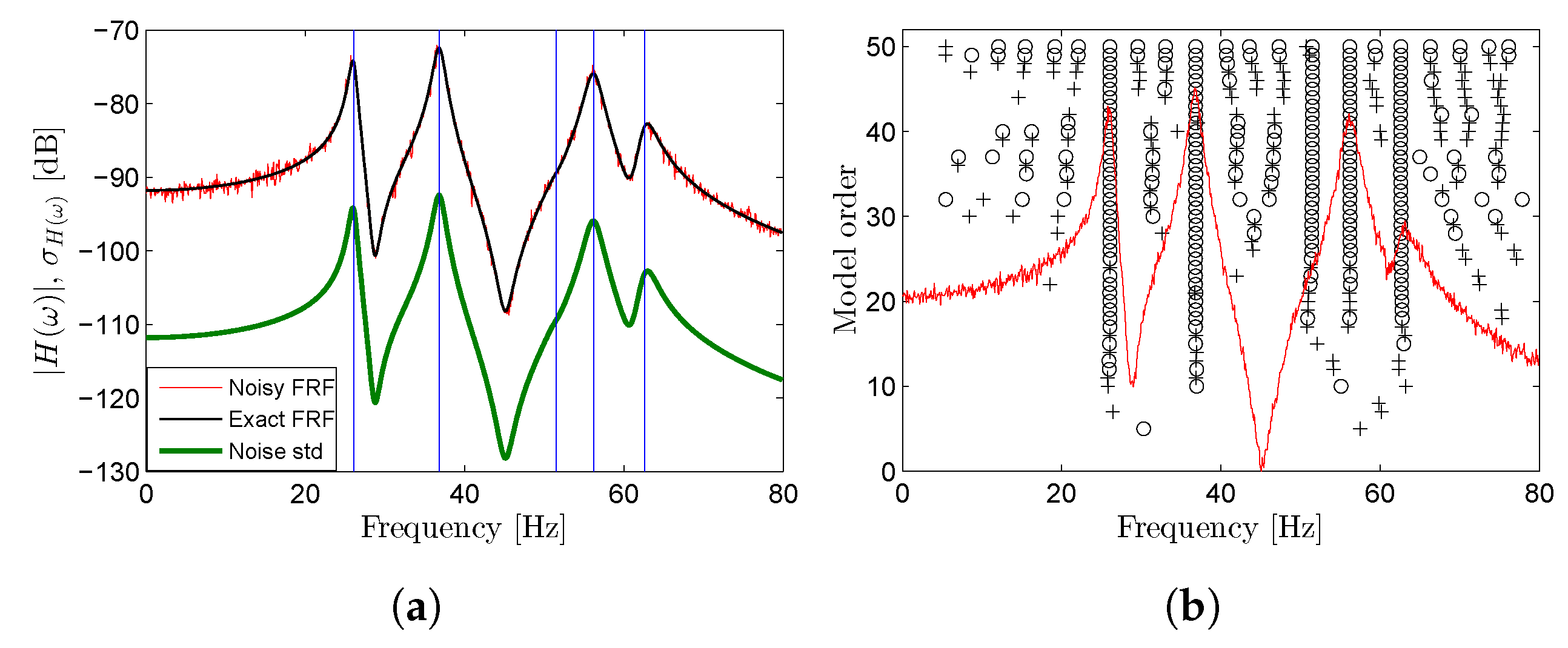
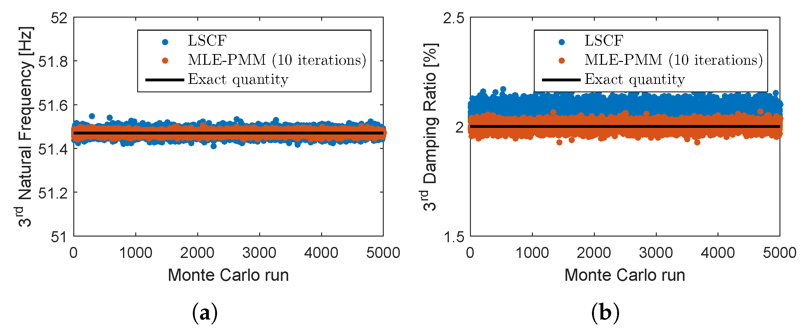
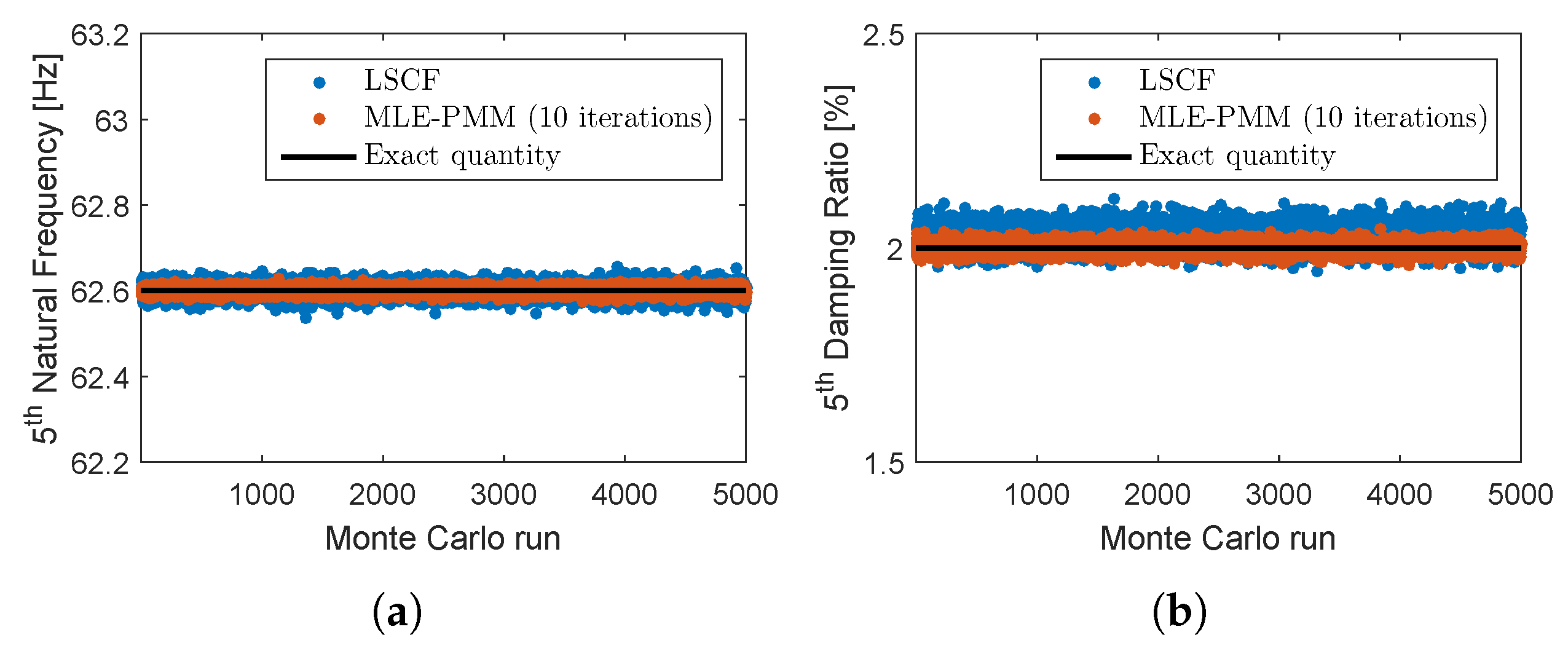
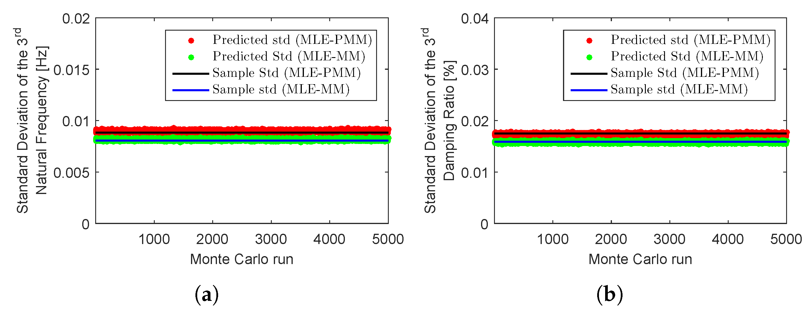
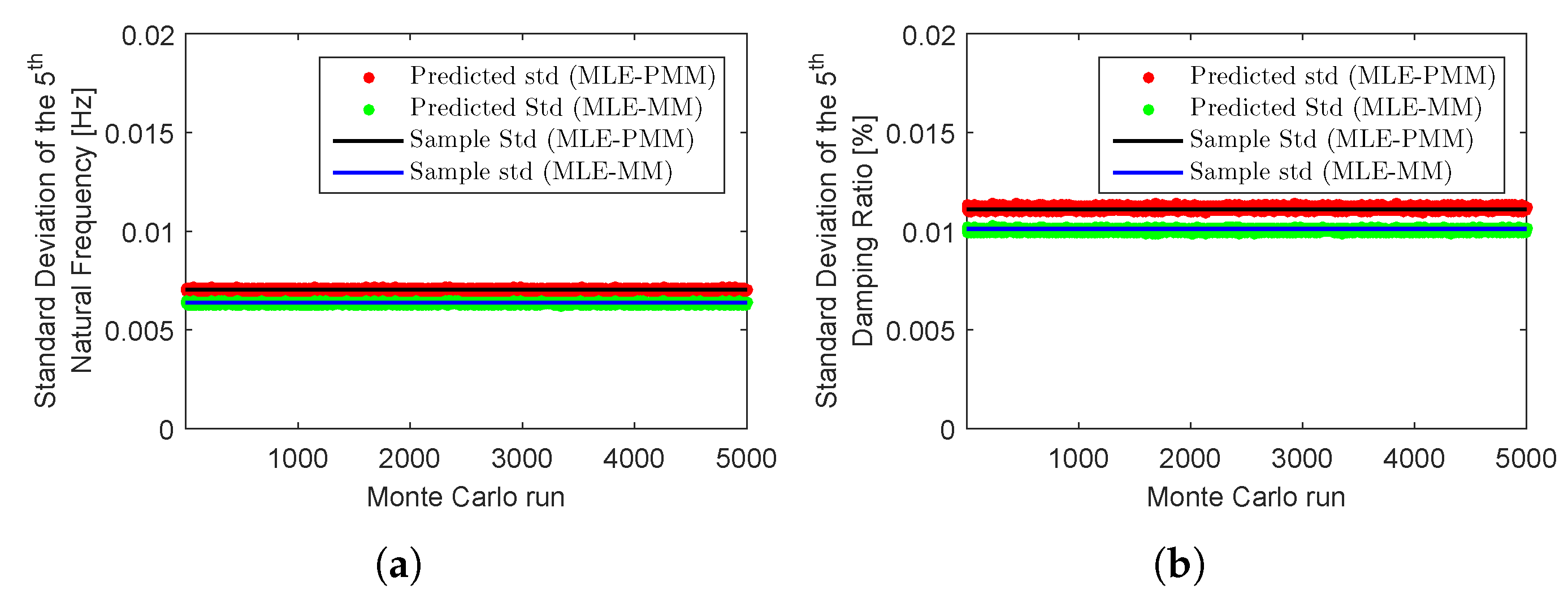
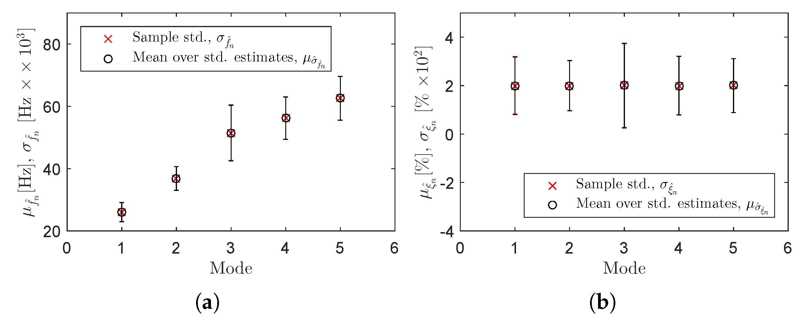
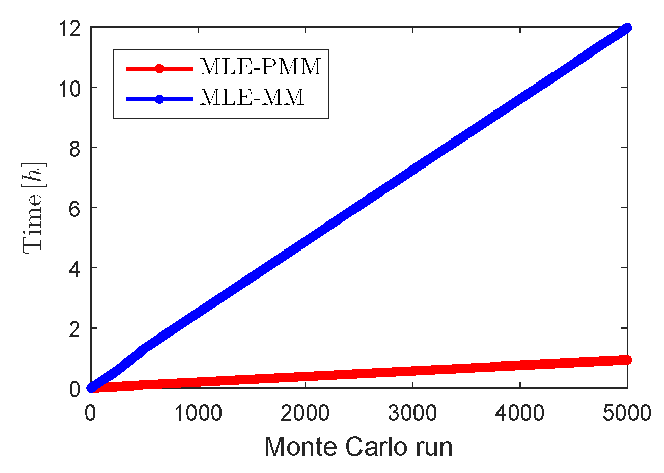
3. Simulated Data Analysis

In order to validate the proposed implementation of the MLE-MM, two examples are analysed. The first consists of a simulated EMA of a five-DOF system and the second corresponds to a lattice tower structure with two pairs of closely spaced modes. In these analyses, the modal parameters together with their uncertainty bounds were estimated using the new MLE-PMM introduced in Section 2.2. The results obtained for both examples are presented in following subsections.

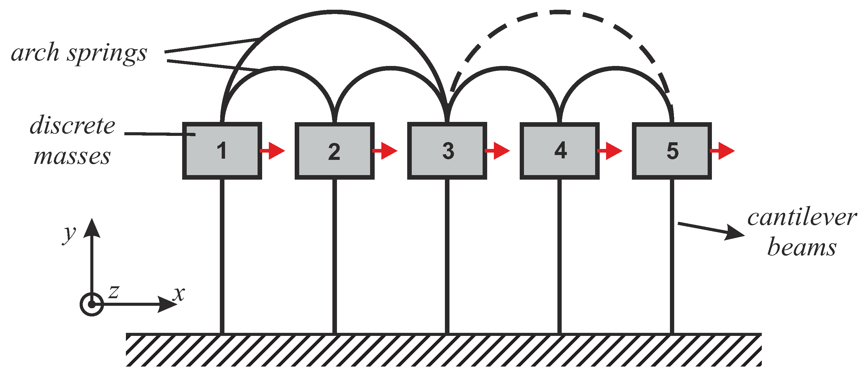
3.1. Five-DOF System

The first example used to validate the ML-based approach discussed in Section 2.2 is illustrated in Figure 2. This system was used in Reference [28] to compare different modal parameter estimation techniques in terms of their sensitivity to statistical errors. It is composed by 5 masses supported by cantilever beams and connected among themselves by arch springs. The exact natural frequencies, damping ratios and modal masses of the system are given in

Table 2. Eigenfrequencies, damping ratios and modal masses of the five-DOF system.

Mode	${\mathit{f}}_{\mathit{n}}$ [Hz]	${\mathit{\xi }}_{\mathit{n}}$ [%]	${\mathit{m}}_{\mathit{i}}$ [Kg]
1	26.06	2	2.52
2	36.84	2	2.97
3	51.47	2	0.90
4	56.21	2	1.09
5	62.60	2	1.05

, whereas the real modes are shown in

Table 3. Real modes of the five-DOF system.

DOF/Mode	1	2	3	4	5
1	0.7147	1.0000	−0.0911	−0.9230	−0.6083
2	0.7166	0.9999	−0.1493	1.0000	−0.1937
3	0.7981	0.2257	0.1554	−0.1518	1.0000
4	0.8518	−0.5166	1.0000	0.1231	−0.3936
5	1.0000	−0.8590	−0.5860	0.0196	−0.2041

. These properties were used to generate the FRFs used in simulated EMA.

The system was excited by a white Gaussian noise at masses 1 and 2 and the responses were measured at all DOFs, resulting in FRF matrix with two columns and five rows. These FRFs were calculated in the frequency range of 0–80 Hz with a resolution of 0.1 Hz. Afterwards, a colored noise was introduced in the FRF matrix with a standard deviation of $10\%$. The noise was added to the real and imaginary parts independently and was calculated as a percentage of the absolute value of the FRF at each frequency line. This was achieved by adding a complex random number to the FRF at each frequency line. This number was computed so that its amplitude is a random number of a normal distribution and its phase is an uniform random number between 0 and $2\pi$ [13].

The exact and noisy element(1,1) of the FRF matrix and the corresponding “exact” standard deviation of the noise are shown in Figure 3a. A set of 5000 FRFs with 800 frequency lines contaminated with noise was generated to perform Monte Carlo simulations in order to assess the efficiency of the proposed MLE-PMM. The modal parameters of each dataset were identified with the LSCF and LSFD estimators and then used as starting values to be optimized by the MLE-PMM algorithm. The identification of each dataset was performed using the full frequency band, that is, with no upper and lower residual terms. Though 1000 Monte Carlo simulations would be more than enough to assess the robustness of the MLE-PMM, a higher number of realizations were performed, in this particular simulation example, to also verify its efficiency in predicting the 95% elliptical confidence regions. A typical stabilization diagram constructed with the LSCF method from the noisy FRF is shown in Figure 3b.

As a final step of the identification process, 10 iterations of the MLE-PMM were performed to optimize the modal parameters of each Monte Carlo dataset and estimate their sample standard deviations. The variation of the LSCF and MLE-PMM estimates for the $3\mathrm{rd}$ and $5\mathrm{th}$ natural frequencies and damping ratios over the Monte Carlo simulations are shown in Figure 4 and Figure 5, respectively.

Analyzing these figures, one verifies that, while no changes can be visually perceived for the estimated natural frequencies with regard to their exact counterparts, a significant improvement in accuracy of the damping ratio estimates after the optimization with MLE-PMM is clearly visible. This conclusion is corroborated by the results presented in

Table 4. Monte Carlo simulation results obtained from the simulated EMA of the five-DOF system: mean natural frequencies and damping rations and their respective relative bias error computed from the LSCF estimates and from the estimates obtained with the MLE-PMM technique after 10 iterations.

Mode	LSCF Estimates				MLE-PMM Estimates (10 Iterations)
	${\mathit{\mu }}_{{\widehat{\mathit{f}}}_{\mathit{n}}}$	Rel.Bias	${\mathit{\mu }}_{{\widehat{\mathit{\xi }}}_{\mathit{n}}}$	Rel.Bias	${\mathit{\mu }}_{{\widehat{\mathit{f}}}_{\mathit{n}}}$	Rel.Bias	${\mathit{\mu }}_{{\widehat{\mathit{\xi }}}_{\mathit{n}}}$	Rel.Bias
	(Hz)	(% $\times {10}^3$)	(%)	(% $\times {10}^2$)	(Hz)	(% $\times {10}^3$)	(%)	(% $\times {10}^2$)
1	26.0603	1.129	2.0449	2.246	26.0600	0.152	1.9998	0.011
2	36.8404	1.131	2.0317	1.585	36.8398	0.425	1.9999	0.004
3	51.4715	2.927	2.0685	3.423	51.4702	0.337	2.0005	0.025
4	56.2125	4.378	2.0274	1.370	56.2100	0.042	1.9999	0.004
5	62.6006	0.934	2.0275	1.373	62.6001	0.216	2.0000	0.002

where the results obtained from the Monte Carlo simulations are compared in terms of mean relative bias error.

One of the main advantages of the MLE-PMM approach herein proposed with regard to the optimization technique described in Reference [19] is that the former takes into account not only the FRFs but also the noise information as primary data and, therefore, apart from the modal parameter estimates, it also predicts the uncertainties on theses estimates. In order to illustrate this capability, the standard deviations of the natural frequencies and damping ratios predicted after 10 iterations of the proposed MLE-PMM for the $3\mathrm{rd}$ and $5\mathrm{th}$ modes in each Monte Carlo run are compared to the respective sample standard deviations in Figure 6 and Figure 7. In these figures, the results obtained with the proposed MLE-PMM are also compared to those from the MLE-MM described in Reference [14]. Similarly to the MLE-PMM, the optimization of the pLSCF estimates with the MLE-MM was also performed with 10 iterations in each Monte Carlo run. It is clear from Figure 6 and Figure 7 that the standard deviations provided by the proposed MLE-PMM are in very good agreement both with their corresponding sample standard deviations and with standard deviation obtained with MLE-MM.

The estimates for the damping ratios obtained after 10 iterations of the MLE-PMM in each Monte Carlo run are plotted as a function of the corresponding natural frequency estimates in Figure 8. Also, in this figure, the ‘classical’ 95% confidence ellipses calculated both with the sample covariance and the mean covariance computed from the estimates obtained with Equation (26) over 5000 Monte Carlo runs are shown. It is clearly seen from such figure that not only the shape of the uncertainty regions defined by the damping ratio and natural frequency estimates but also the estimated 95% confidence ellipses are in good agreement with the corresponding sample covariance ellipses.

These results also demonstrate the MLE-PMM capability of providing very accurate confidence regions for the optimized modal properties. The MLE-PMM capability of predicting the sample standard deviations for all the identified modes is illustrated in Figure 9 and

Table 5. Monte Carlo simulation results obtained from the simulated EMA of the five-DOF system: comparison between the sample standard deviations and those predicted in a typical Monte Carlo run with the proposed MLE-PMM after 10 iterations.

Estimator	Mode	Sample Std.		Mean Over the Std. Estimates		Rel. Difference (${\mathit{d}}_{\mathit{\sigma },\widehat{\mathit{\sigma }}}$)
		${\mathit{\sigma }}_{{\widehat{\mathit{f}}}_{\mathit{n}}}$ (Hz × 103)	${\mathit{\sigma }}_{{\widehat{\mathit{\xi }}}_{\mathit{n}}}$ (% × 102)	${\widehat{\mathit{\sigma }}}_{{\widehat{\mathit{f}}}_{\mathit{n}}}$ (Hz × 103)	${\widehat{\mathit{\sigma }}}_{{\widehat{\mathit{\xi }}}_{\mathit{n}}}$ (% × 102)	${\mathit{d}}_{{\mathit{\sigma }}_{{\widehat{\mathit{f}}}_{\mathit{n}}},{\widehat{\mathit{\sigma }}}_{{\widehat{\mathit{f}}}_{\mathit{n}}}}$ (%)	${\mathit{d}}_{{\mathit{\sigma }}_{{\widehat{\mathit{\xi }}}_{\mathit{n}}},{\widehat{\mathit{\sigma }}}_{{\widehat{\mathit{\xi }}}_{\mathit{n}}}}$ (%)
MLE-PMM	1	3.04	1.20	3.10	1.18	1.74	2.23
	2	3.80	1.03	3.80	1.04	0.05	0.38
	3	8.83	1.75	8.97	1.73	1.60	1.05
	4	6.74	1.20	6.81	1.21	1.12	1.20
	5	7.04	1.11	7.02	1.12	0.29	0.51
MLE-MM	1	3.01	1.19	3.06	1.16	1.53	2.15
	2	3.70	1.01	3.70	1.01	0.20	0.33
	3	8.07	1.59	8.15	1.58	1.01	0.49
	4	5.34	0.98	5.47	0.97	2.39	0.35
	5	6.37	1.01	6.35	1.00	0.36	0.68

. In the former, the sample standard deviations computed from the 5000 sets of estimates obtained with the Monte Carlo simulations are compared to the means of the standard deviation estimates provided by the MLE-PMM. In the latter, this comparison is established, in terms of relative difference, both for the MLE-PMM and the MLE-MM estimates. Analysing these results, one verifies that the MLE-PMM provided accurate predictions for the sample standard deviation of all the identified modes, which are as well in good agreement with the MLE-MM estimates.

Although it is verified from Figure 6 and Figure 7 and from Table 5 that the MLE-MM provides slightly lower uncertainty bounds for optimized estimates, the MLE-PMM algorithm is significantly less time consuming. This is verified in Figure 10 where the performance of the ML-PMM algorithm is compared, in terms of time consumed over the performed Monte Carlo simulations, to its ML-MM counterpart. The significant difference in processing time between the two algorithms is explained by the fact that the dimensions of the system matrices obtained with the MLE-PMM is significantly lower than those of the MLE-MM.

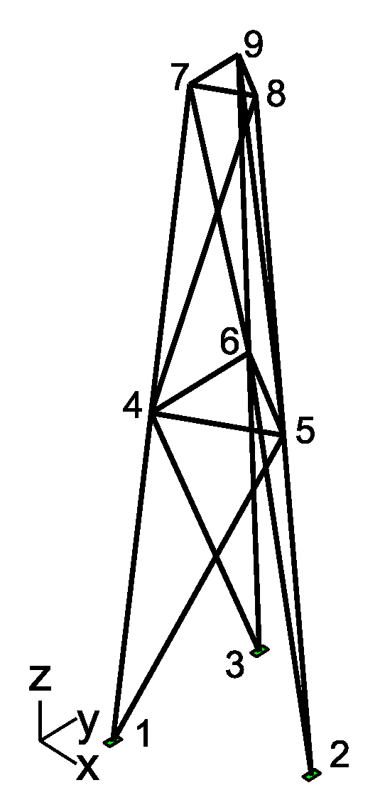
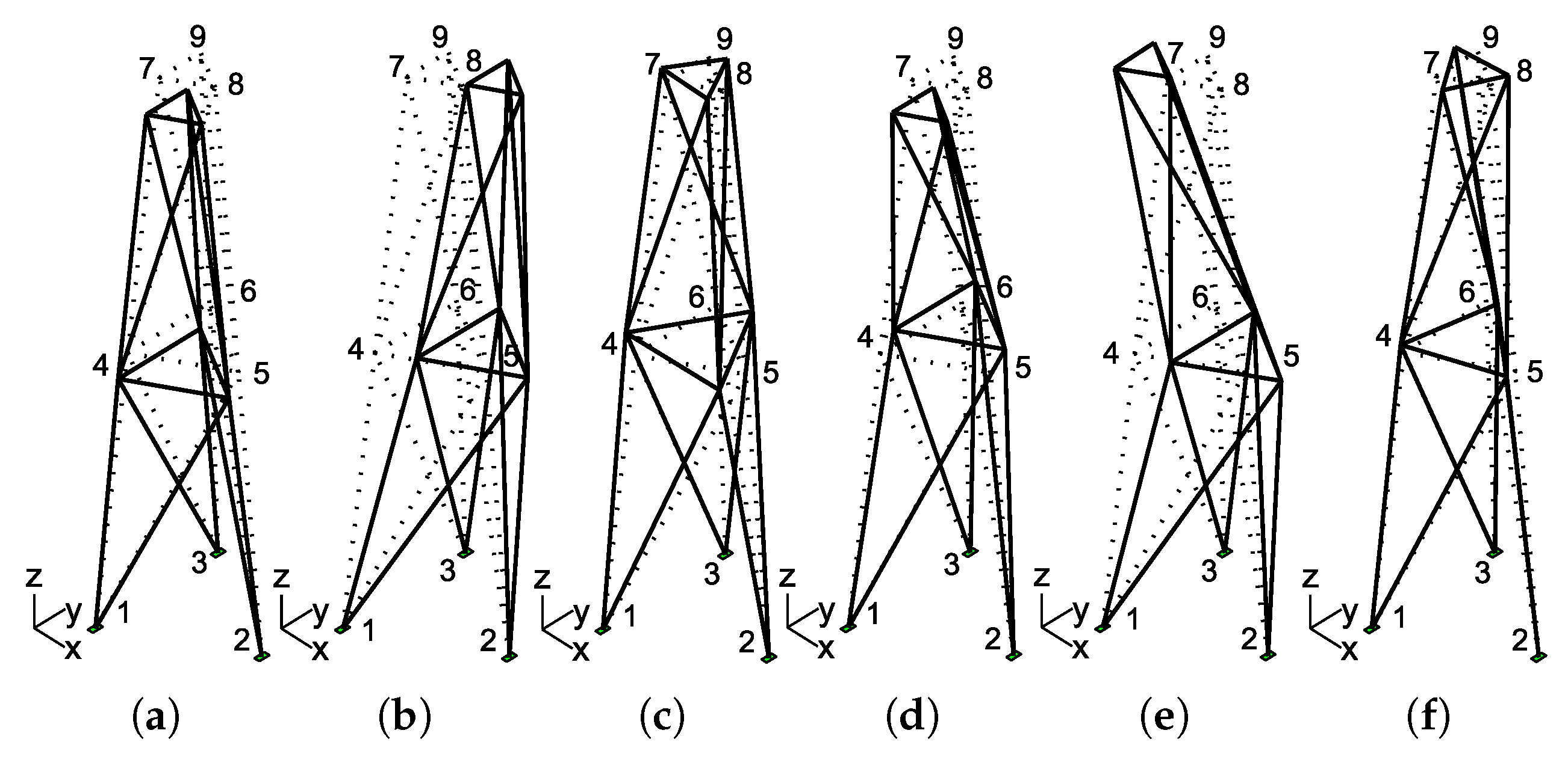
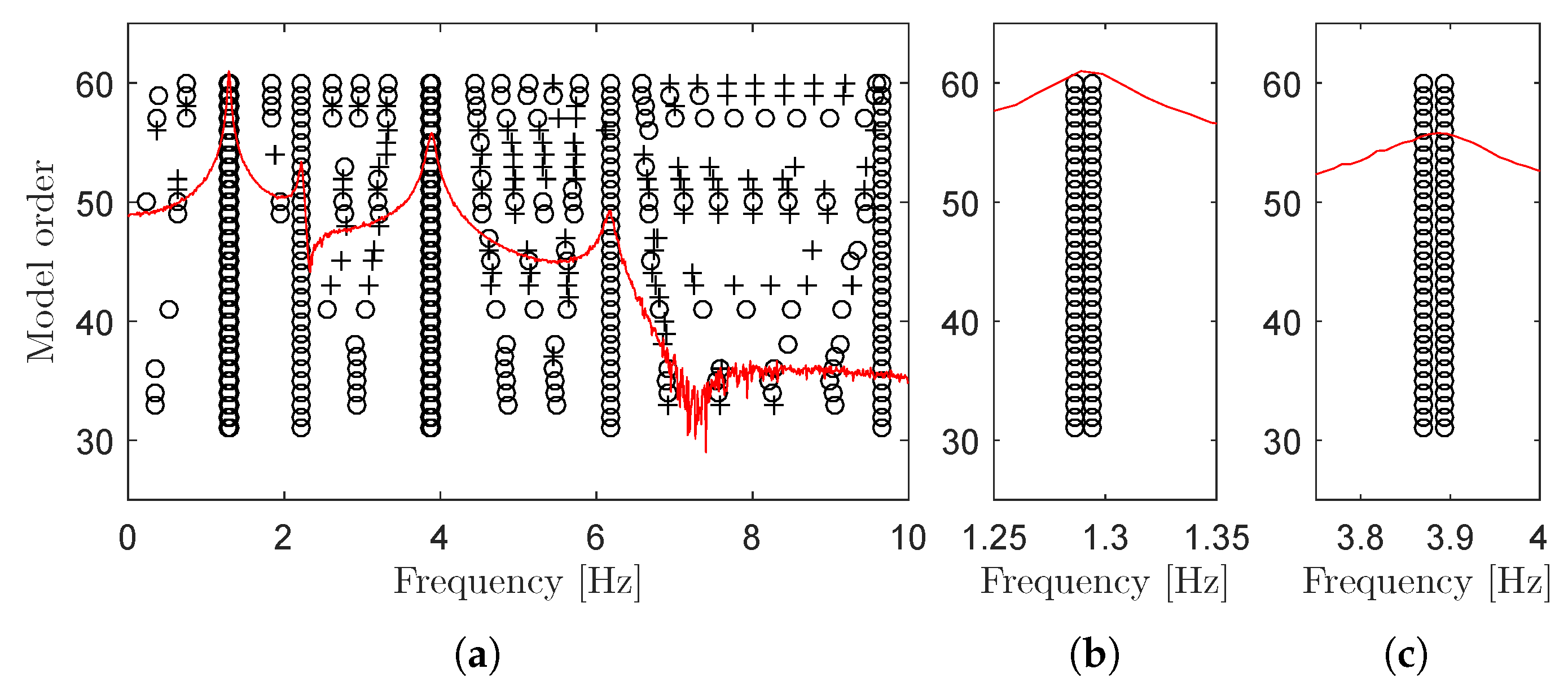
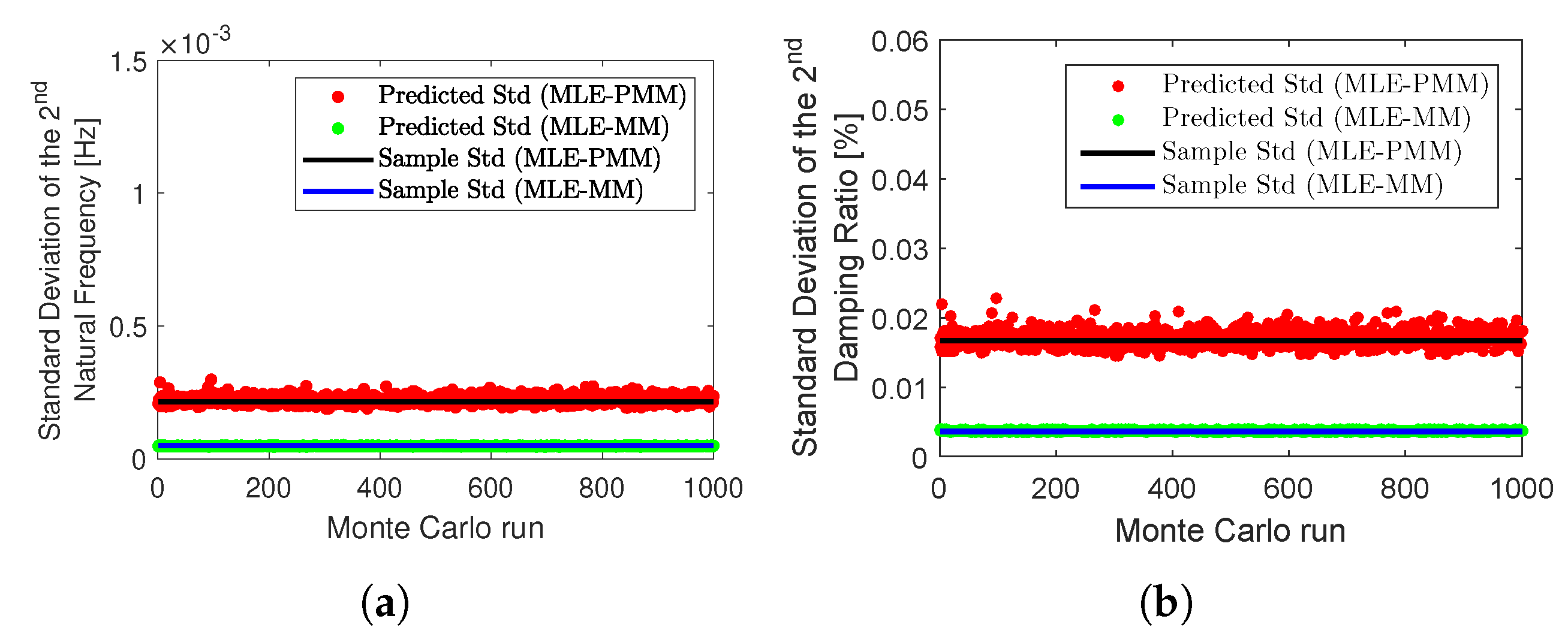
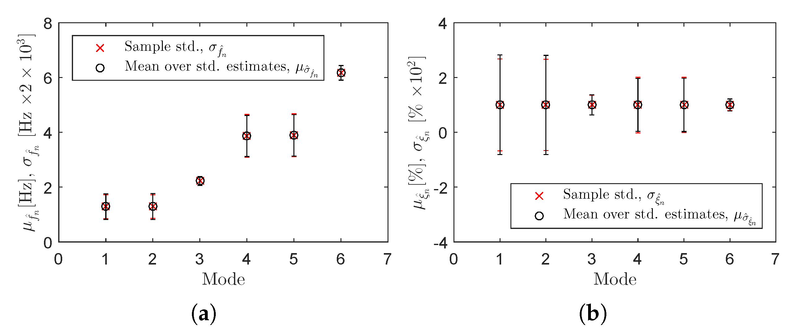
3.2. Lattice Tower Example

The second simulated example used to validate the ML approach discussed in Section 2.2 consists of a finite element model which is illustrated in Figure 11. The example consists of a lattice tower structure constituted by two segments of equal height and by variable equilateral triangular sections. The lower section is scaled with regard to the upper one by a factor of 2. This model is composed by beam elements with 6 DOFs per node. The nodes of the foundations are clamped and the others have 3 DOFs: two translations in x and y and one rotation around z-axis; and the remaining DOFs are set equal to zero. These settings result in a FE model with a total of $N_m=18$ DOFs.

The symmetry of the structure was slightly broken by defining different geometry and materials to the column elements in order to simulate the behaviour of tower-like structures, which normally present very closely spaced of bending modes. The real mode shapes of the tower structure are shown in

Table 6. Real modes of the lattice tower structure used in simulation examples.

DOF/Mode	1	2	3	4	5	6
1	0.4468	−0.6874	0.3127	0.3392	0.6939	0.1024
2	−0.6972	−0.4527	−0.1825	−0.6996	0.3094	−0.0583
3	−0.1535	0.0972	0.6919	0.1836	0.1287	−0.0468
4	0.4489	−0.6965	0.0014	0.3186	0.6843	0.0022
5	−0.7059	−0.4370	0.3573	−0.7115	0.3235	0.1151
6	0.1269	0.1106	0.6946	−0.1849	0.0980	−0.0492

. The first 6 modal configurations and the corresponding modal parameters of the FE model of the lattice tower are presented in Figure 12 and

Table 7. Modal configurations of the FE model of the lattice structure.

Mode	Type	${\mathit{f}}_{{\mathit{n}}_{\mathit{i}}}$ [Hz]	${\mathit{\xi }}_{{\mathit{n}}_{\mathit{i}}}$ [%]	${\mathit{m}}_{\mathit{i}}$ [Kg]
1	$1\mathrm{st}$ bending mode in Y direction (BY1)	1.2869	1.0	2608.8271
2	$1\mathrm{st}$ bending mode in X direction (BX1)	1.2937	1.0	2592.8286
3	$1\mathrm{st}$ torsional mode (T1)	2.2251	1.0	281.0965
4	$2\mathrm{nd}$ bending mode in Y direction (BY2)	3.8713	1.0	1431.1279
5	$2\mathrm{nd}$ bending mode in X direction (BX2)	3.8932	1.0	1410.8619
6	$2\mathrm{nd}$ torsional mode (T2)	6.1745	1.0	54.2551

, respectively.

The structural damping, on the other hand, is modelled as the special case of proportional damping by setting the damping coefficients of all modes equal to 1%. The structure was excited, independently, at node 8 in x and y-direction and at node 9 in y-direction with white noise inputs. The simulated responses were measured in acceleration at the 6 DOFs indicated in Figure 13. By assuming that the two triangular sections behave as rigid diaphragms, the measured outputs are enough to yield the modal configurations of the structure. The FRF matrix with 6 rows and 3 columns was calculated in the frequency range of 0–10 Hz with a resolution of 10 mHz. Afterwards, a colored noise was introduced in the FRF matrix with a standard deviation of $5\%$.

The noise was added to the FRFs following the same procedure described in the previous example. The exact and noisy element(1,1) of the FRF matrix, the corresponding exact standard deviation of the noise as well as the exact natural frequencies are shown in Figure 14. A set of 1000 FRFs with 1000 frequency lines contaminated with noise was generated to perform Monte Carlo simulations in order to assess the efficiency of the proposed MLE-PMM when dealing with closely spaced modes. In the first step of the identification of each dataset, a stabilisation diagram was constructed with the LSCF technique from the measured FRFs and the approach based on Hierarchical Clustering described in References [29,30] was subsequently used to automatically identify the physical modal properties.

A typical stabilization diagram constructed by identifying models with order ranging from 30 to 60 is represented in Figure 15. Next, the FRF matrix was synthesized from the estimates obtained with the LSCF technique was then used as starting guess by the MLE-PMM. Finally, a total of 20 iterations were performed, both to optimize the estimates obtained with LSCF in the first step and to compute confidence intervals of the optimized estimates. Differently from the previous application example, a higher number of iterations was used in these simulations to secure the convergence of the cost function $l\left(\Theta \right)$. This difference is explained by the fact that the system being optimized in this particular simulation example comprises vibration modes with closely spaced natural frequencies and, therefore, the ML estimator needs to iterate more times to reach convergence. Similarly to the previous application example, the optimization with the MLE-PMM was carried out using again the full frequency band, i.e., with no out-of-band modes.

The variation of the natural frequency and damping ratio estimates for modes 2 and 5 obtained both with the LSCF and MLE-PMM over the Monte Carlo simulations are shown in Figure 16 and Figure 17 and the results obtained in terms of relative bias error for all the identified modes are synthesized in

Table 8. Monte Carlo simulation results obtained from the simulated EMA of the lattice tower structure: mean natural frequencies and damping rations and their respective relative bias error computed from the LSCF estimates and from the estimates obtained with the MLE-PMM technique after 20 iterations.

Mode	LSCF Estimates				MLE-PMM Estimates (20 Iterations)
	${\mathit{\mu }}_{{\widehat{\mathit{f}}}_{\mathit{n}}}$	Rel.Bias	${\mathit{\mu }}_{{\widehat{\mathit{\xi }}}_{\mathit{n}}}$	Rel.Bias	${\mathit{\mu }}_{{\widehat{\mathit{f}}}_{\mathit{n}}}$	Rel.Bias	${\mathit{\mu }}_{{\widehat{\mathit{\xi }}}_{\mathit{n}}}$	Rel.Bias
	(Hz)	(% $\times {10}^3$)	(%)	(% $\times 10$)	(Hz)	(% $\times {10}^3$)	(%)	(% $\times 10$)
1	1.2869	0.294	1.0000	0.003	1.2869	0.050	1.0003	2.816
2	1.2937	0.839	1.0020	20.201	1.2937	0.272	1.0000	0.334
3	2.2251	0.107	1.0001	0.723	2.2251	0.001	0.9999	1.282
4	3.8712	0.154	1.0007	6.951	3.8713	0.209	1.0002	2.035
5	3.8932	0.805	1.0000	0.014	3.8932	0.002	0.9998	1.957
6	6.1745	0.119	1.0004	3.687	6.1745	0.059	1.0000	0.001

.

By comparing the results obtained before and after the optimization with MLE-PMM shown in this table, it is verified that no significant reduction in terms of the bias error was obtained after 20 iterations of the MLE-PMM with regard to the LSCF estimates. The mean of standard deviation estimates for the natural frequencies and damping ratios of modes 2 and 5 predicted by the proposed MLE-PMM after 20 iterations are compared to their respective sample standard deviations in Figure 18 and Figure 19. By inspecting these figures, one verifies that, even in case of closely spaced modes, the MLE-PMM provides very good estimates for the sample standard deviations.

These results are also verified in Figure 20 and

Table 9. Monte Carlo simulation results obtained from the simulated EMA of the five-DOF system: comparison between the sample standard deviations and those predicted in a typical Monte Carlo run with the proposed MLE-PMM after 20 iterations.

Estimator	Mode	Sample Std.		Mean Over the Std. Estimates		Rel. Difference (${\mathit{d}}_{\mathit{\sigma },\widehat{\mathit{\sigma }}}$)
		${\mathit{\sigma }}_{{\widehat{\mathit{f}}}_{\mathit{n}}}$ (Hz × 103)	${\mathit{\sigma }}_{{\widehat{\mathit{\xi }}}_{\mathit{n}}}$ (% × 102)	${\widehat{\mathit{\sigma }}}_{{\widehat{\mathit{f}}}_{\mathit{n}}}$ (Hz × 103)	${\widehat{\mathit{\sigma }}}_{{\widehat{\mathit{\xi }}}_{\mathit{n}}}$ (% × 102)	${\mathit{d}}_{{\mathit{\sigma }}_{{\widehat{\mathit{f}}}_{\mathit{n}}},{\widehat{\mathit{\sigma }}}_{{\widehat{\mathit{f}}}_{\mathit{n}}}}$ (%)	${\mathit{d}}_{{\mathit{\sigma }}_{{\widehat{\mathit{\xi }}}_{\mathit{n}}},{\widehat{\mathit{\sigma }}}_{{\widehat{\mathit{\xi }}}_{\mathit{n}}}}$ (%)
MLE-PMM	1	0.22	1.68	0.22	1.70	2.00	1.52
	2	0.21	1.67	0.22	1.70	3.35	2.08
	3	0.08	0.36	0.08	0.37	0.26	1.30
	4	0.39	1.01	0.37	0.97	4.54	4.45
	5	0.39	1.01	0.38	0.97	3.33	3.97
	6	0.13	0.21	0.13	0.22	3.05	3.27
MLE-MM	1	0.05	0.38	0.05	0.37	1.54	1.56
	2	0.05	0.36	0.05	0.37	2.86	2.88
	3	0.08	0.33	0.08	0.34	0.86	1.44
	4	0.11	0.27	0.11	0.28	2.07	3.21
	5	0.11	0.28	0.11	0.28	2.10	0.64
	6	0.13	0.20	0.13	0.21	1.66	3.46

, where the sample standard deviations of all the identified natural frequencies and damping ratios are compared to those predicted by the MLE-PMM. In Figure 18 and Figure 19 and in Table 9, the estimates for the standard deviations provided by the MLE-PMM are also compared to the estimates obtained with MLE-MM proposed by Reference [14] after 20 iterations. From this comparison it is concluded that, even though the MLE-PMM provides very accurate estimates for the uncertainty bounds of its optimized modal parameter estimates, these uncertainty intervals are significantly higher than those provided by the MLE-MM. This leads to the conclusion that, in case of closely spaced modes, the optimisation with the MLE-PMM is not as efficient as in case of reasonably or well separated modes.

4. Conclusions

In this paper, a novel ML-based estimator formulated in pole-residue modal model is proposed. Just like any other ML-based approach, the MLE-PMM introduced in this paper requires a good starting guess to assure convergence over the performed Gauss-Newton iterations. Despite the fact that any LS-based identification technique can be used to provide the starting guess, the proposed ML approach is combined with the LSCF estimator to retain the multi-reference information and improve the accuracy of the LS estimates. The idea of combining the ML-PMM with LSCF estimator aims at taking advantage of the particular features of each estimators, that is, (i) the fast modal parameter estimation obtained with the latter; and (ii) the numerical stability of the former. It was verified that, when combined with the LSCF estimator, the MLE-PMM is capable of improving the accuracy of the LSCF estimates and providing confidence intervals for the optimized estimates.

The main advantage of the proposed MLE-PMM with regards to the MLE-MM is that, due to the reduced dimension of the system matrices, it is significantly less time consuming, as demonstrated in the first application example presented in Section 3.1. Another distinguishing feature of the derived ML approach is that, due to the parametrization used in its formulation, the variances of the natural frequencies and damping coefficients are estimated directly from the Jacobian matrix. Therefore, the use of additional linearization formulas is avoided if one is only interested on these variances. The main disadvantages, however, are in fact, related to the limitations of modal model in pole residue form. These disadvantages include: (1) difficulty of distinguishing between close spaced modes; (2) difficulty in accurately synthesizing the FRF matrix once the mode shapes and modal participation factor vectors are estimated from the modal residues by means of the singular value decomposition; and (3) difficulty in fully optimizing the LSCF modal parameter estimates used as starting guess in case of closely spaced modes.

When dealing with reasonably or well separated modes, however, it is observed that MLE-PMM performs very well when compared to it modal model based counterpart. Two application examples were used to validate the proposed ML-based estimator. The first consisted of well separated whereas the second of closely spaced modes. From the simulations with former, it was demonstrated the ability of the MLE-PMM technique to significantly reduce the bias error of the LSCF estimates and predict the uncertainties for the optimized estimates. This is demonstrated by the results presented in Table 4 and Table 5. From the simulations with the latter, it was verified (as shown in Table 8 and Table 9) that, even in case of closely spaced modes, the proposed MLE-PMM was capable of reducing the bias error of the LSCF estimates and providing reliable predictions for the confidence intervals of the optimized estimates.

References

1. Guillaume, P.; Verboven, P.; Vanlanduit, S.; Van-der-Auweraer, H.; Peeters, B. A Poly-reference Implementation of the Least-squares Complex Frequency-domain Estimator. In Proceedings of the 21st International Modal Analysis Conference (IMACXXI), Kissimmee, FL, USA, 3–6 February 2003. [Google Scholar]
2. Peeters, B.; Van-der-Auweraera, H.; Guillaume, P.; Leuridana, J. The PolyMAX frequency-domain method: A new standard for modal parameter estimation? Shock Vib. 2004, 1, 395–409. [Google Scholar] [CrossRef]
3. Peeters, B. System Identification and Damage Detection in Civil Engineering. Ph.D. Thesis, Katholieke Universiteit Leuven, Leuven, Belgium, 2000. [Google Scholar]
4. Peeters, B.; Van-der-Auweraer, H.; Vanhollebeke, F.; Guillaume, P. Operational modal analysis for estimating the dynamic properties of a stadium structure during a football game. Shock Vib. 2007, 14, 283–303. [Google Scholar] [CrossRef]
5. Maia, N.; He, L.; Lin, S.; To, U. Theoretical and Experimental Modal Analysis; Research Studies Press Ltd.: London, UK, 1998. [Google Scholar]
6. De-Troyer, T.; Guillaume, P.; Pintelon, R.; Vanlanduit, S. Fast calculation of confidence intervals on parameter estimates of least-squares frequency-domain estimators. Mech. Syst. Signal Process. 2009, 23, 261–273. [Google Scholar] [CrossRef]
7. De-Troyer, T.; Guillaume, P.; Steenackers, G. Fast variance calculation of polyreference least-squares frequency-domain estimates. Mech. Syst. Signal Process. 2009, 23, 1423–1433. [Google Scholar] [CrossRef]
8. Reynders, E.; Pintelon, R.; De-Roeck, G. Uncertainty bounds on modal parameters obtained from stochastic subspace identification. Mech. Syst. Signal Process. 2008, 22, 948–969. [Google Scholar] [CrossRef]
9. Döhler, M.; Lam, X.-B.; Mevel, L. Uncertainty quantification for modal parameters from stochastic subspace identification on multi-setup measurements. Mech. Syst. Signal Process. 2013, 36, 562–581. [Google Scholar] [CrossRef]
10. Reynders, E.; Maes, K.; De-Roeck, G. Uncertainty quantification in operational modal analysis with stochastic subspace identification: Validation and applications. Mech. Syst. Signal Process. 2016, 66–67, 13–30. [Google Scholar] [CrossRef]
11. El-Kafafy, M.; Guillaume, P.; De-Troyer, T.; Peeters, B. A Frequency—Domain Maximum Likelihood Implementation using the modal model formulation. In Proceedings of the 16th IFAC Symposium on System Identification the International Federation of Automatic Control, Brussels, Belgium, 11–13 July 2012. [Google Scholar]
12. El-Kafafy, M. Design and Validation of Improved Modal Parameter Estimators. Ph.D. Thesis, Department of Mechanical Engineering, Vrije Universiteit Brussel, Brussels, Belgium, 2013. [Google Scholar]
13. Peeters, B.; El-Kafafy, M.; Guillaume, P. The new PolyMAX Plus method: Confident modal parameter estimation even in very noisy cases. In Proceedings of the 2012 Conference on Noise and Vibration Engineering (ISMA), Leuven, Belgium, 17–19 September 2012. [Google Scholar]
14. El-Kafafy, M.; De-Troyer, T.; Peeters, B.; Guillaume, P. Fast maximum-likelihood identification of modal parameters with uncertainty intervals: A modal model–based formulation. Mech. Syst. Signal Process. 2013, 37, 422–439. [Google Scholar] [CrossRef]
15. El-Kafafy, M.; De-Troyer, T.; Guillaume, P. Fast maximum-likelihood identification of modal parameters with uncertainty intervals: A modal model formulation with enhanced residual term. Mech. Syst. Signal Process. 2014, 48, 49–66. [Google Scholar] [CrossRef]
16. Diord, S.; Magalhães, F.; Cunha, A.; Caetano, E. High spatial resolution modal identification of a stadium suspension roof: Assessment of the estimates uncertainty and of modal contributions. Eng. Struct. 2017, 135, 117–135. [Google Scholar] [CrossRef]
17. El-kafafy, M.; Guillaume, P.; Peeters, B.; Marra, F.; Coppotelli, G. Advanced frequency-domain modal analysis for dealing with measurement noise and parameter uncertainty. In Proceedings of the 19th International Modal Analysis Conference (IMACXXX), Jacksonville, FL, USA, 30 January–2 February 2012. [Google Scholar]
18. El-Kafafy, M.; Peeters, B.; Guillaume, P.; De-Troyer, T. Constrained maximum likelihood modal parameter identification applied to structural dynamics. Mech. Syst. Signal Process. 2016, 72–73, 567–589. [Google Scholar] [CrossRef]
19. Balmès, E. Frequency domain identification of structural dynamics using the pole-residue parametrization. In Proceedings of the 1996 International Modal Analysis Conference (IMAC), Orlando, FL, USA, 12–15 February 1996. [Google Scholar]
20. Heylen, W.; Lammens, S.; Sas, P. Modal Analysis Theory and Testing, 2nd ed.; Mechanical Engineering, Katholieke Universiteit Leuven: Leuven, Belgium, 1998; Volume 1. [Google Scholar]
21. Guillaume, P.; Verboven, P.; Vanlanduit, S. The new PolyMAX Plus method: Confident modal parameter estimation even in very noisy cases. In Proceedings of the 23rd International Seminar on Modal Analysis, Leuven, Belgium, 16–18 September 1998. [Google Scholar]
22. Cauberghe, B. Applied Frequency-Domain System Identification in the Field of Experimental and Operational Modal Analysis. Ph.D. Thesis, Department of Mechanical Engineering, Vrije Universiteit, Brussel, Belgium, 2004. [Google Scholar]
23. Pintelon, R.; Schoukens, J. System Identification: A Frequency Domain Approach, 1st ed.; IEEE Press: Piscataway, NJ, USA, 2001; Volume 1. [Google Scholar]
24. Schoukens, J.; Pintelon, R. System Identification: A Frequency Domain Approach, 1st ed.; Pergamon Press: London, UK, 1991; Volume 1. [Google Scholar]
25. Kailath, T. Linear Systems, 1st ed.; Prentice-Hall: Upper Saddle River, NJ, USA, 1998; Volume 1. [Google Scholar]
26. Pintelon, R.; Guillaume, P.; Schoukens, J. Uncertainty calculation in (operational) modal analysis. Mech. Syst. Signal Process. 2007, 21, 2359–2373. [Google Scholar] [CrossRef]
27. Verboven, P. Frequency-Domain System Identification for Modal Analysis. Ph.D. Thesis, Department of Mechanical Engineering, Vrije Universiteit Brussel, Brussels, Belgium, 2002. [Google Scholar]
28. Böswald, M.; Göge, D.; Füllekrug, U.; Govers, Y. A review of experimental modal analysis methods with respect to their applicability to test data of large aircraft. In Proceedings of the International Conference on Noise and Vibration Engineering, Leuven, Belgium, 18–20 September 2006. [Google Scholar]
29. Diord, S.; Magalhães, F.; Cunha, A.; Caetano, E.; Martins, N. Automated modal tracking in a football stadium suspension roof for detection of structural changes. Struct. Control Health Monit. 2017, 24, e2006. [Google Scholar] [CrossRef]
30. Amador, S.D.R. Uncertainty Quantification in Operational Modal Analysis and Continuous Monitoring of Special Structures. Ph.D. Thesis, Department of Civil Engineering, Faculty of Engineering of University of Porto, Porto, Portugal, 2015. [Google Scholar]
Figure 1. Chart flow of the identification with the combined LSCF-MLE-PMM.
Applsci 09 03120 g001
Figure 2. Five-DOF system connected with arch springs [28].
Applsci 09 03120 g002
Figure 3. Element(1,1) of the FRF matrix contaminated with 10 % noise: exact (black line) and noisy (red line) FRF, noise standard deviation (green line) and exact natural frequencies (vertical lines) (a); and stabilization diagram (with ‘∘’ denoting a pole with stable frequency and damping and ‘+’ a pole with stable frequency only) constructed with the LSCF estimator by identifying common denominator polynomial models with order ranging from 1 to 50 (b).
Applsci 09 03120 g003
Figure 4. Monte Carlo simulation results for the 3 rd identified natural frequency (a) and damping ratio (b): exact quantity (solid black line), LSCF estimates (blue dots) and MLE-PMM estimates after 10 iterations (red dots).
Applsci 09 03120 g004
Figure 5. Monte Carlo simulation results for the 5 th identified natural frequency (a) and damping ratio (b): exact quantity (solid black line), LSCF estimates (blue dots) and MLE-PMM estimates after 10 iterations (red dots).
Applsci 09 03120 g005
Figure 6. Monte Carlo simulation results for the five-DOF system example with 10% noise: sample standard deviation of the natural frequencies (a) and damping ratios (b) estimated for the 3 rd mode both with the MLE-PMM and MLE-MM [14] and their corresponding standard deviation estimates obtained after 10 iterations.
Applsci 09 03120 g006
Figure 7. Monte Carlo simulation results for the five-DOF system example with 10% noise: sample standard deviation of the natural frequencies (a) and damping ratios (b) estimated for the 5 th mode both with the MLE-PMM and MLE-MM [14] and their corresponding standard deviation estimates obtained after 10 iterations.
Applsci 09 03120 g007
Figure 8. Covariances on the estimates for the natural frequencies and damping ratios obtained with the MLE-PMM for all modes of the 5-DOF system: estimates obtained after 10 iterations of the MLE-PMM over the Monte Carlo realizations (blue dots); 95% elliptical confidence regions obtained from the sample covariance, Cov ( f ^ n , ξ ^ n ) (continuous black line); and 95% elliptical confidence regions obtained from the mean over the covariance estimates provided by the MLE-PMM over the Monte Carlo simulations (dashed red line).
Applsci 09 03120 g008
Figure 9. Monte Carlo simulation results for the identified natural frequencies (a) and damping ratios (b): sample mean and standard deviation (black line) and mean and standard deviation predicted after 10 iterations of MLE-PMM (red line) from a typical Monte Carlo dataset.
Applsci 09 03120 g009
Figure 10. Time consumed by MLE-PMM (red line) and MLE-MM [14] (blue line) algorithms over the Monte Carlo runs.
Applsci 09 03120 g010
Figure 11. Finite element model of the tower example used in the simulated analysis.
Applsci 09 03120 g011
Figure 12. First six mode shapes of the tower structure: 1 st bending mode in Y direction (BY1) (a), 1 st bending mode in X direction (BX1) (b), 1 st torsional mode (T1) (c), 2 nd bending mode in Y direction (BY2) (d), 2 st bending mode in X direction (BX2) (e) and 2 nd torsional mode (T2) (f).
Applsci 09 03120 g012
Figure 13. Sensors and measured directions.
Applsci 09 03120 g013
Figure 14. Element(1,1) of the FRF matrix contaminated with 5 % noise: exact and noisy FRF, noise standard deviation and exact natural frequencies (vertical lines) (a); and details of the close spaced modes around 1.29 Hz (a) and 3.88 Hz (b).
Applsci 09 03120 g014
Figure 15. Typical stabilization diagram constructed with the LSCF for model orders ranging from 30 to 60.
Applsci 09 03120 g015
Figure 16. Monte Carlo simulation results for the 2 nd identified natural frequency (a) and damping ratio (b): exact quantity (solid black line), LSCF estimates (blue dots) and MLE-PMM estimates after 20 iterations (red dots).
Applsci 09 03120 g016
Figure 17. Monte Carlo simulation results for the 5 th identified natural frequency (a) and damping ratio (b): exact quantity (solid black line), LSCF estimates (blue dots) and MLE-PMM estimates after 20 iterations (red dots).
Applsci 09 03120 g017
Figure 18. Monte Carlo simulation results for the lattice tower example with 5% of noise level: sample standard deviation of the natural frequencies (a) and damping ratios (b) (solid line) estimated for the 2 nd mode and the corresponding standard deviations predicted from a typical Monte Carlo dataset after 20 iterations of the MLE-PMM (dots).
Applsci 09 03120 g018
Figure 19. Monte Carlo simulation results for the lattice tower example with 5% of noise level: sample standard deviation of the natural frequencies (a) and damping ratios (b) (solid line) estimated for the 5 th mode and the corresponding standard deviations predicted from a typical Monte Carlo dataset after 20 iterations of MLE-PMM (dots).
Applsci 09 03120 g019
Figure 20. Monte Carlo simulation results for the identified natural frequencies and damping ratios: sample (black line) and predicted (red line) means and standard deviations of natural frequencies (a) and damping ratios (b) provided by the proposed MLE-PMM method after 20 iterations.
Applsci 09 03120 g020