A Low Overhead Mapping Scheme for Exploration and Representation in the Unknown Area

Abstract

The grid map, representing area information with the number of cells, is a widely used mapping scheme for mobile robots and simultaneous localization and mapping (SLAM) processes. However, the tremendous amount of cells in a grid map for a detailed map representation results in overheads for memory space and computing paths in mobile robots. Therefore, to overcome the overhead of the grid map, this study proposes a new low overhead mapping scheme which the authors call as the Rmap that represents an area with variable sizes of rectangles instead of the number of cells in the grid map. This mapping scheme also provides an exploration path for obtaining new information for the unknown area. This study evaluated the performance of the Rmap in real environments as well as in simulation environments. The experiment results show that the Rmap can reduce the overhead of a grid map. In one of our experimental environments, the Rmap represented an area with 85% less memory than the grid map. The Rmap also showed better coverage performance compared with other previous algorithms.

1. Introduction

Simultaneous localization and mapping (SLAM) is considered the primary process required by many mobile robot applications such as exploration, cleaning, patrol, and autonomous driving robots [1,2]. In general, it has a hectic process because localization and mapping are performed simultaneously and iteratively. Therefore, various studies have been carried out to reduce the calculation overhead of the SLAM [1,2,3,4,5,6,7,8,9,10,11]. The extended Kalman filter SLAM (EKF-SLAM) has attempted to reduce localizing computation through feature-based landmarks using the mean and covariance matrices [3,4]. The fast-SLAM has tried to reduce the calculation for recognizing locations by using a particle filter called the Rao-Blackwellised filter [5,6]. Another fast-SLAM study has improved performance by applying a nonlinear transformed unscented Kalman filter [7]. The distributed particle SLAM (DP-SLAM) maintains a joint probability distribution for recognizing map and robot positions using particle filters [8]. These approaches improved the performance of SLAM through their ideas.

However, most SLAM algorithms using the grid map still require many computations to make accurate maps. The grid map has the advantage of accurately representing the real environment on a cell by cell basis [9,10,11]. In Figure 1a is the environment and all areas are split into a grid, as shown in Figure 1b. On the other hand, a grid map requires remaining the tremendous amount of cells to represent the map correctly. However, the structure of a grid map requires two-dimensional data such as an array. This data consists of all cells from $x_0$, $y_0$ to $x_{map of width}$, $y_{map of height}$. This format means that the map should remain a rectangular structure, regardless of the shape of the map. For example, to represent a completed map of a triangle, the grid map creates a rectangular map that matches the array structure containing all the vertices of the triangle. Here, the area of the array created for only the representation, except for the triangle map, is not the information of a map, although it must always be loaded when SLAM uses the map. These problems cause SLAM to do more calculations.

A topological mapping method has been proposed to overcome problems of the grid map, as shown in Figure 1c. It is a way to create a graph based on landmarks such as walls, corners, and obstacles [12,13]. This method represents an area as a node. The node is the area where the mobile robot can move. If an area and the other area are connected, these two areas are connected using the edge. The edge is the path that can move in these two areas. Therefore, this map representation method efficiently uses memory to use the map through nodes and edges [14]. The topological map efficiently reduces memory. However, there is a problem that the detailed movement of the mobile robot is difficult because the information on the map is insufficient.

Therefore, a hybrid mapping scheme has been proposed, which has both grid map information and topological map efficiency. The approximate cell decomposition algorithm uses a recursive method to continue subdividing the cells and connects divided cells through the edge as a topological map [15]. Additionally, a path planning method using approximate cell decomposition has been proposed [16]. However, there is a limit to maps that must be known in advance to divide the cells by a recursive process in this method. The SLAM without the information of the area in advance cannot use this method.

In this paper, a new mapping scheme is proposed for reducing overheads in the SLAM, which the authors called the Rmap. It uses rectangles instead of cells of the grid map to enable efficient exploration while performing the SLAM on unknown areas.

The rest of this paper is organized as follows. Section 2 introduces the Rmap scheme in detail. Section 3 shows the performance evaluation results of the Rmap. Finally, conclusions are discussed in Section 4.

2. A New Mapping Scheme of Rmap

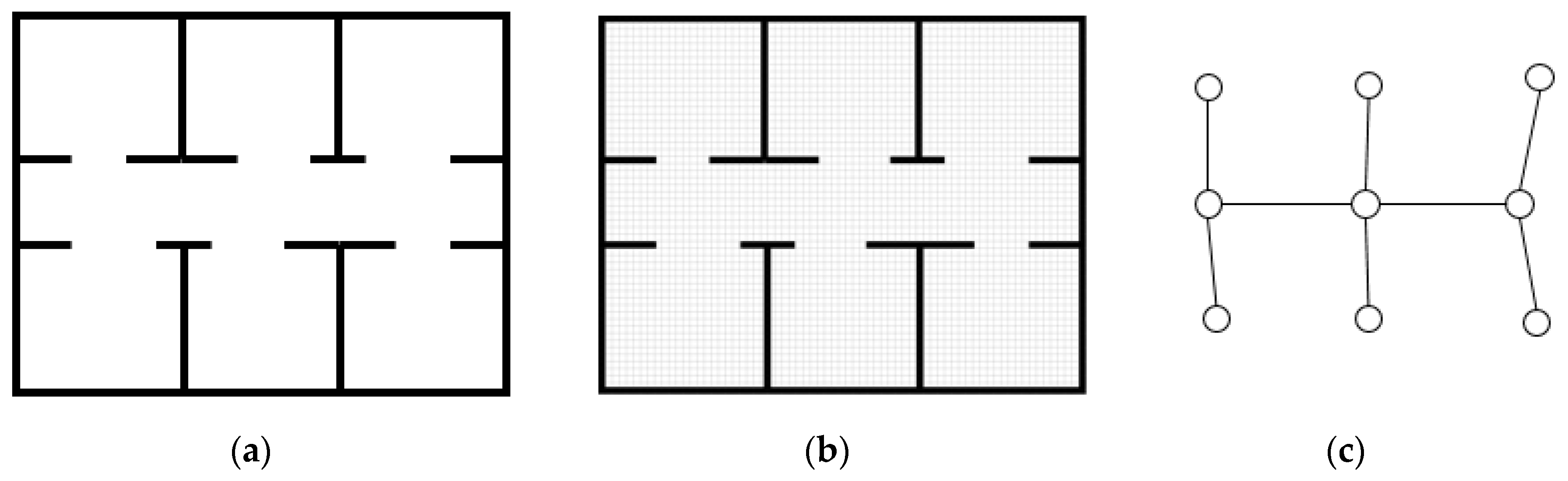
2.1. The Framework of Rmap

In this section, the entire framework of the Rmap and detailed algorithms are introduced. The Rmap consists of several modules, such as the initial map setting, the minimal bounding rectangle (MBR) creation, R1 selection, the map update, exploration, and the map extension check module as shown in Figure 2. This mapping framework works with the localization module of the SLAM algorithm.

The initial map setting is a step of collecting initial information when the mobile robot is located in an unknown environment, as shown in Figure 3a. At this step, the robot generates an initial map about the given environment through a one-rotation. The white area of Figure 3b shows the initial sensing data obtained by the rotation of the robot.

The MBR creation module creates a minimal bounding rectangle (MBR), as shown in the blue dotted box of Figure 3b. The MBR is the smallest rectangle that can contain all the areas acquired in the initial map setting and all the newly sensing data in the exploration.

The R1 selection is the next step to obtain R1 from the MBR. R1 is the largest rectangle that can be created in the occupied area of the MBR. This study uses the rectangle tiling algorithm to get R1. The rectangle tiling is a mathematical algorithm for finding configurable rectangles in a grid [17]. For a rectangle with a height of m x width n, the whole rectangle candidates can be calculated within the created MBR region by the rectangle tiling algorithm, as shown in Equation (1).

$$N\left(m,n\right)={\displaystyle \sum }_{i=0}^{m-1}{\displaystyle \sum }_{j=0}^{n-1}\left(m-i\right)\left(n-j\right)=\frac{1}{4}m\left(m+1\right)n\left(n+1\right)$$

(1)

A similar problem to the set covering problem [18] is finding the largest rectangle among these candidates. The set covering problem is one of the representative Karp’s 21 NP-complete problems in the field of computer science [19]. This study uses the greedy method to calculate the size of all the rectangular candidates to obtain R1, R2, R3, ..., Rn in size order. Through this method, the largest rectangle R1 can be chosen. An example of the creation of R1 is the green box in Figure 3c. Then, the R1 information is updated to the map.

After updating the R1 information, the robot needs to explore the area for getting new information. This study designed the exploration step, and it is performed to plan and move the robot. The primary exploration policy is to follow the updated R1′s boundary line, as shown in the red line in Figure 3c. At this time, the robot moves from the current position to the boundary of R1 by the shortest path. When the robot performs the exploration step, it can explore new areas like the increased white area of Figure 3d. The Rmap scheme using this moving policy can plan an exploration path that minimizes a duplicate path in an unknown environment.

The map extension check step verifies that the robot has obtained a new area in the exploration step. If the robot has acquired a new area, the Rmap process starts from the MBR creation step, as shown in Figure 3d after combining the previously acquired area with the new area. In the case of not acquiring a new map, the Rmap process returns to the R1 selection step and selects R1 from the previously collected area, except the updated area in the Rmap. If R1 is no longer created after this iteration process, it means that the mapping is completed.

Algorithm 1. Rmap Algorithm

1 2 3 4 5 6 7 8 9 10 11 12 13 14 15 16 17 18 19 20

Begin Let R = {r1, r2, …, rn} is a set of rectangles Let E = {e1, e2, …, en} is a set of edges of adjacent rectangles Let Map=<R,E> be a map generated by Rmap algorithm Let MBR be the Minimum Bounding Rectangle $\mathrm{InitialMapSetting}$ with robot rotation $\mathit{Loop}until there is no more unkown area:$ $\hspace{1em}\mathrm{MBR}\leftarrow \mathrm{MBR}\mathrm{Creation}\left(\mathrm{sensed}\mathrm{data}\right)$ $\hspace{1em}\hspace{1em}\mathrm{Rectangle}\mathrm{list} \leftarrow \mathrm{RectangleTiling} \left(\mathrm{MBR}\right)$ $\hspace{1em}\hspace{1em}\mathrm{R}1 \leftarrow \mathrm{R}1\mathrm{Selection}\left(\mathrm{Rectangle}\mathrm{list}\right)$ $\hspace{1em}\mathrm{Map}\leftarrow \mathrm{MapUpdate}\left(R1\right)$ $\hspace{1em}\hspace{1em}\mathrm{sensed}\mathrm{data}\leftarrow \mathrm{Exploration} \mathrm{with}\mathrm{following}\mathrm{the}\mathrm{borderline}\mathrm{of}\mathrm{R}1$ $\hspace{1em}\hspace{1em}\mathrm{Map}\mathrm{Extension}\mathrm{Check}\left(\mathrm{sensed}\mathrm{data}\right)$   If there is no new sensed data outside MBR area      Goto line 11 R1 Selection step   Else      Goto line 9 MBR Creation step   End If EndOfLoop End

Algorithm 1 shows the entire procedure of the Rmap scheme described so far. The Rmap algorithm works until there is no more unknown area after initialization. The Map, generated by the Rmap algorithm, consists of R and E, where R is a set of rectangles, the E is a set of edges of adjacent rectangles. In the initialize stage, the initial map setting step initializes the Map using sensed data. After the initialization, the map building process repeats until the map is completed. The MBR is generated in the MBR creation step based on the sensed data. Next, the rectangle list is created using the rectangle tiling algorithm on the generated MBR. The R1 selection step selects R1, the largest rectangle in this rectangle list. The selected R1 is updated to the Map through the map update step. The exploration step explores the updated R1, where the default value is R1′s borderline following policy. The map extension check step checks the existence of the newly acquired information by comparing the sensed data. If there is new information, this process goes to line 9 MBR creation step. Otherwise, this process goes to line 11 R1 selection process. The Rmap can complete the map building through iteration of this process.

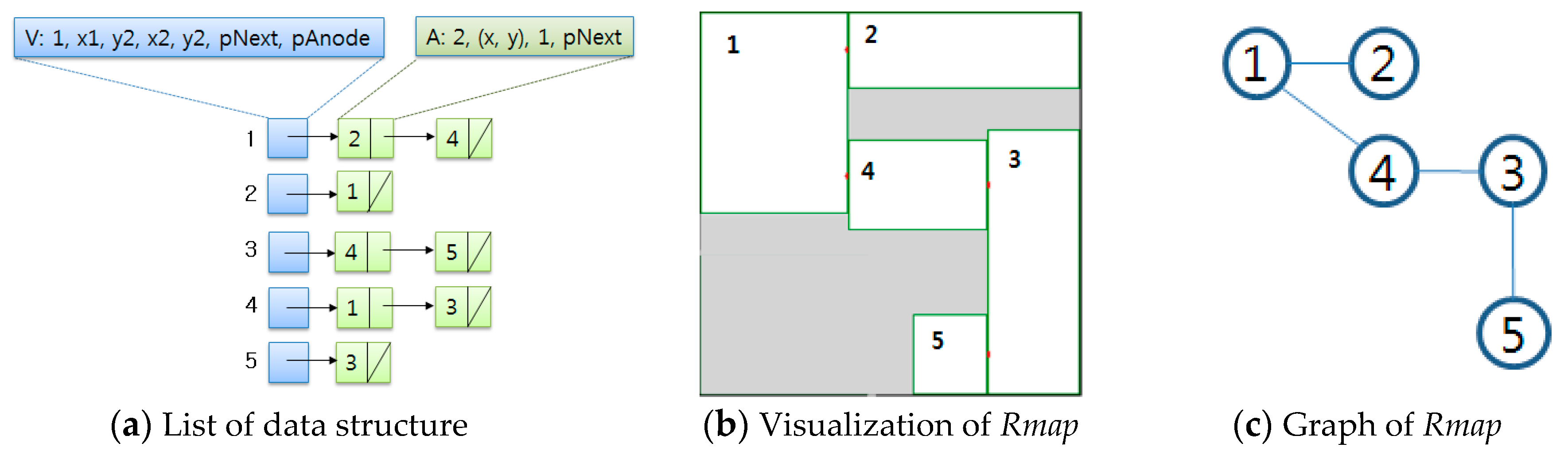
2.2. Data Structure of Rmap

This study’s basic idea is to use the rectangles that bind pixels instead of the pixel units of the grid map, as shown in Figure 4. These rectangles of the Rmap for performing SLAM allow the map to be maintained and used with much less memory compared to the grid map. Therefore, these rectangles are managed as nodes and links of the graph. Thus, the Rmap can be expressed as follows:

$$Rmap=\left\{VNode, ANode\right\}$$

(2)

The data structure of the Rmap consists of the VNode and the ANode, as shown in Expression (2). The VNode is vertex node and contains information of the rectangles in the Rmap. The ANode means the adjacent node that contains information of the adjacent nodes of the VNode. The VNode includes the identification information (ID) of the nodes, the coordinate information (CoodinateR) of the nodes, the next node information (pNext), and the list information (pANode) of the adjacent nodes, as shown in Expression (3).

$$VNode=\left\{ID, CoordinateR, pNext, pAnode\right\}$$

(3)

The ANode as shown in Expression (4) includes the identification information (ID) of the adjacent nodes—the adjacent node intermediate contact information (ACP: adjacent center point), the distance value (nDistance) of the adjacent nodes, the list information (pNext) of the adjacent nodes.

$$ANode=\left\{ID, ACP, nDistance, pNext\right\}$$

(4)

The Rmap has a graph structure of the VNode and the ANode, as shown in (a) of Figure 5, and the VNode of area 1 is connected with the ANode of 2 and 4. The (b) of Figure 5 visualizes the data structure of (a) and shows area 1 connected with area 2 and area 4, and also indicates the ACP in the adjacent parts of each area. Finally, (c) is a graph representation of the data structure (a). The map data can be constructed through this logic, which enables efficient memory usage.

2.3. Path Planning Scheme Using Rmap

In general, the SLAM algorithms and mapping algorithms do not take into account path planning algorithms. This is because the path planning is thought to be another problem. However, the robot’s path planning has an important influence on how quickly the robot completes the map for the entire area in collecting information for the actual drawing of a map.

Most of the path planning algorithms based on the grid map are completed by calculating pixels. Therefore, they require a considerable amount of operations because every pixel on the map needs to be considered every time a movement event occurs. Therefore, the path planning operation on the grid map causes overheads in the SLAM.

However, this study’s mapping scheme efficiently addresses this calculation overhead for path planning using the graph structure of the Rmap, as shown in Figure 5c. By using the ANode and the VNode information of the Rmap, the shortest path between two points can be calculated. For example, when the robot has located someplace in rectangle 1 in Figure 5b, if the robot needs to go to some position in rectangle 3, the path can be calculated as (1- > 4- > 3) using Dijkstra’s shortest path algorithm [20]. After calculating the path, the robot can move to the target using the ACP information of the selected path. As previously described, the ACP is a center point between two adjacent rectangles. Thus, for this case, the robot can start from its current place to the ACP point of rectangle 1 and 4. Then, it can move to the ACP point of rectangles 4 and 3. Finally, the mobile robot can move to the target position in rectangle 3. As seen in this example, if the ACP information of the Rmap is being used, the robot can move to any place in the map very quickly and safely.

The ACP is created and maintained when the Rmap is updated. There are two cases of ACP creation. One is the horizontal case, and the other is the vertical overlapping case as shown in Figure 6. The Equation for creating the ACP is as follows:

$$CoordinateR\left(A\right) :A\left(A_{x1},A_{y1},A_{x2},A_{y2}\right)$$

(5)

$$CoordinateR\left(B\right) :B\left(B_{x1},B_{y1},B_{x2},B_{y2}\right)$$

(6)

$$ACP\left(x,y\right)=\left(\frac{A_{x1}+B_{x2}}{2},A_{y2}\right)$$

(7)

$$ACP\left(x,y\right)=\left(A_{x2},\frac{B_{y1}+B_{y2}}{2}\right)$$

(8)

The Equations (5) and (6) represent the coordinates of the two points that make up the rectangle in the VNode of the two adjacent maps A and B. Equation (7) can calculate the ACP in the case of a horizontal overlapping case, and Equation (8) is for calculating the ACP in the case of vertical overlapping. The ACP is stored in the ANode information.

2.4. Applied Usage Case of Rmap for Coverage

The Rmap also can be used for coverage application with slight modifications in the unknown environment. The coverage refers to the algorithm of visiting all of the areas at least once. The cleaning robot is a representative example of coverage application.

For applying the Rmap to coverage application, some part of the Rmap algorithm needs to be changed. The Rmap in coverage cases works the same until the R1 rectangle is selected. After getting the R1 rectangle in the Rmap algorithm, the robot has to follow the boundary line of the R1 rectangle to obtain more information about the unknown area. However, for coverage, the robot needs to visit the whole R1 rectangle area. For covering the R1 rectangle area, the Boustrophedon path algorithm [21] can be adopted. The Boustrophedon path algorithm is a well-known algorithm in the coverage field. The Boustrophedon path means a zigzag style movement, as shown in Figure 7. While covering the R1 rectangle using the Boustrophedon path algorithm, the modified exploration policy also obtains new information of the unknown area for a map update. After covering the R1 rectangle area, the rest of the processes are the same as the original Rmap scheme. Algorithm 2 shows the modified version of the Rmap for coverage application. As previously described, the algorithm has changed only for the exploration mechanism after updating the R1 rectangle. For the coverage case, the Boustrophedon path algorithm instead of the R1′s borderline following is used for the exploration step.

Algorithm 2. Modified Rmap Algorithm for Coverage

1 2 3 4 5 6 7 8 9 10 11 12 13 14 15 16 17 18 19 20

Begin Let R = {r1, r2, …, rn} is a set of rectangles Let E = {e1, e2, …, en} is a set of edges of adjacent rectangles Let Map=<R,E> be a map generated by Rmap algorithm Let MBR be the Minimum Bounding Rectangle $\mathrm{InitialMapSetting}$ with robot rotation $\mathit{Loop} until there is no more unkown area:$ $\hspace{1em}\mathrm{MBR}\leftarrow \mathrm{MBR}\mathrm{Creation}\left(\mathrm{sensed}\mathrm{data}\right)$ $\hspace{1em}\hspace{1em}\mathrm{Rectangle}\mathrm{list} \leftarrow \mathrm{RectangleTiling} \left(\mathrm{MBR}\right)$ $\hspace{1em}\hspace{1em}\mathrm{R}1 \leftarrow \mathrm{R}1\mathrm{Selection} \left(\mathrm{Rectangle}\mathrm{list}\right)$ $\hspace{1em}\mathrm{Map}\leftarrow \mathrm{MapUpdate}\left(\mathrm{R}1\right)$ $\hspace{1em}\hspace{1em}\mathrm{sensed}\mathrm{data}\leftarrow \mathrm{Exploration} \mathrm{with}\mathrm{following}\mathrm{the}\mathrm{BoustrophedonPath}\mathrm{of}\mathrm{R}1$ $\hspace{1em}\hspace{1em}\mathrm{Map}\mathrm{Extension}\mathrm{Check}\left(\mathrm{sensed}\mathrm{data}\right)$   If there is no new sensed data outside MBR area      Goto line 11 R1 Selection step   Else      Goto line 9 MBR Creation step   End If EndOfLoop End

3. Experiments

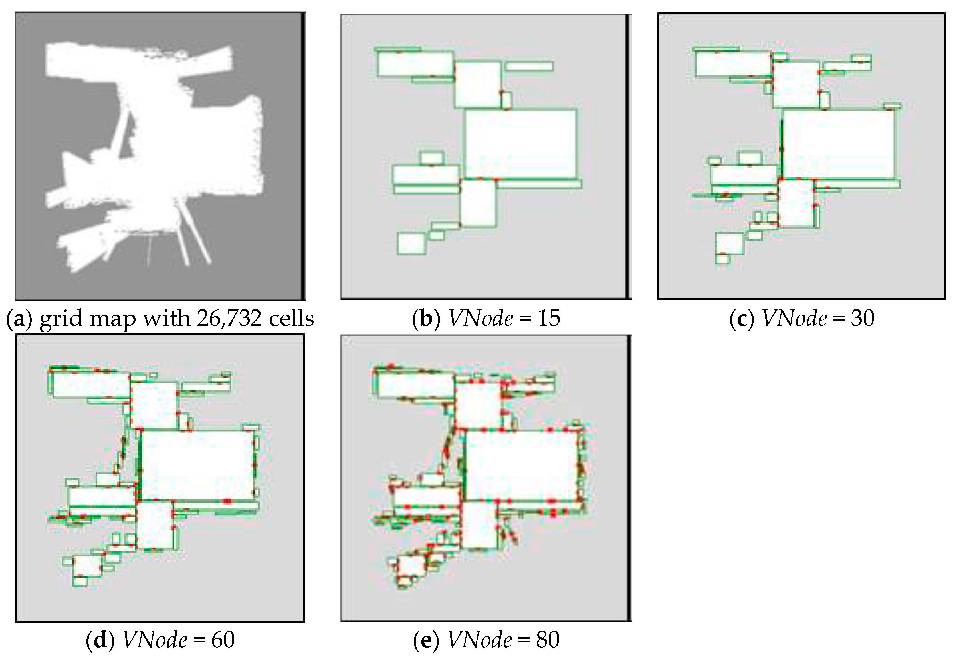
3.1. Experiment Environments

This study evaluated the performance of the Rmap in two environments: The simulation environment and the real environment. The memory efficiency of the Rmap was evaluated in a simulation environment using a Player/Stage simulator. The Rmap algorithm was implemented into the Player/Stage. Moreover, the grid map generated by DP-SLAM was used for comparison, as shown in Figure 8b.

After the simulation, the coverage performance of the Rmap in real environments was evaluated. Figure 8c is the actual indoor layout of the house for the experiments. For the practical experiments, the authors built a robot with the S3C6410 board, URG-04LX-UG01 laser sensor, and two DC motors, as shown in Figure 8d.

3.2. The Memory Efficiency of Rmap

In this section, the memory efficiency of the Rmap compared with the grid map is presented. For comparison, the simulated environment map of Figure 8a generated by the Player/Stage was used. The environment has an area of 22.4 m × 24.1 m. Figure 8b is the grid map from the DP-SLAM algorithm for the environment of Figure 8a. The grid map consists of 215,936 cells with a 5 cm resolution.

Figure 9 shows the results of the Rmap representation for the simulated environment of Figure 8a. Moreover,

Table 1. The numerical results of the memory efficiency experiment.

Results	(a)	(b)	(c)	(d)
The number of rectangles (n)	19	50	113	522
The size of the minimum rectangle (m2)	1.015	0.25	0.05	0.01
The number of ACP	23	78	136	477
Similarity compared to the grid map (%)	92	95	97	99
Elapse Time (sec) performed in 2 Ghz CPU	0.875	1.063	1.375	3.281

enumerates the detailed experiment results. The Rmap achieved a 92% similarity compared to the grid map with only 19 nodes. The similarity means the percentage of the occupied area of the Rmap compared with the area of the grid map. Figure 9a through to (d) show the accuracy of the map increases as the number n of the rectangles increases. As shown in Figure 9d and Table 1d, the map shows 99% similarity with the grid map in 522 rectangles. Compared with the 215,936 cells of the grid map, this is a dramatically reduced number of nodes for showing the same quality of the map.

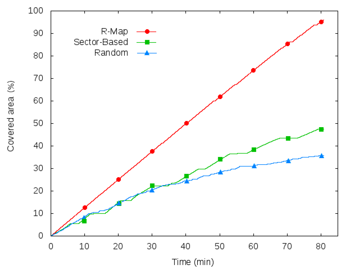
3.3. The Coverage Performance Rmap

The performance of the applied case of the Rmap for coverage was measured. This study implemented the Rmap algorithm to the robot as in Figure 8d. The Rmap was integrated with the DP-SLAM algorithm for mapping. Additionally, other coverage algorithms, such as the sector-based and random coverage algorithms were implemented for comparison. The sector-based coverage algorithm is an algorithm that corrects for poor sensing by dividing the space into sectors and improving the localization on a sector [22]. The random coverage algorithm visits the area randomly as the words. It is simple to implement and it is a widely used an algorithm for many cleaning robots. The experiments were conducted in the actual environment of Figure 8c. That is a blueprint of some house and the inside area of the red line is the actual target area that has an area of approximately 8 m × 13 m.

Figure 10a shows the grid map output from the DP-SLAM. The grid map also shows some outer information of the area through the open doors. It represents the area with 26,732 cells. Figure 10b–e show the process of map building of the Rmap by the number of the VNode. As the number of VNode increases, the quality of the map also increases. With only 80 VNodes, the map shows a very similar quality to the map with the grid map of the previous section.

The graph of Figure 11 shows the coverage performance of the Rmap compared with the other algorithms. The covered area was calculated by comparing the total area and the area visited by the robot in the real environment. For eighty minutes, the Rmap visited almost 95% of the whole area, the sector-based algorithm visited 48%, and the random coverage algorithm visited only 36%. From analyzing the experiment results, the rate of overlapped visits for the area was only 2% for the Rmap algorithm. On the other hand, the rate for sector-based algorithm was 21%, and the random coverage algorithm was 62%. The Rmap algorithm showed the best performance for coverage.

In addition, the performance of the Rmap was evaluated in another extreme case of an environment using the simulator, as shown in Figure 12a. The Rmap, proposed in this paper, built a map using the number of rectangles. Therefore, this approach can have a disadvantage for the rounded environment. Therefore, to prove the robustness of the Rmap scheme, this study added an extreme case of an environment which had many rounded curves inside in it. The environment has an area of 4 m × 4 m. The Rmap scheme shows a quick increase of the covered area to 80% in contrast to other algorithms, as shown in Figure 12b. Thereafter, the slower increasing rate of the covered area is shown because the robot moves using the Boustrophedon path from the generated small rectangles. After all, the Rmap achieved the best-covered area of 98%.

4. Conclusions

In this paper, the Rmap algorithm that improves the performance of the grid map was proposed. The Rmap can represent an area of similar quality to the grid map with a relatively small number of rectangles. The Rmap also can guide an exploration path for obtaining new information in the unknown area. This study also showed an applied case of the Rmap for the coverage application. Compared to the previous mapping algorithms, the Rmap showed better memory efficiency and coverage performance for the unknown area.

This experiment results mean that our Rmap scheme can improve the overheads caused by the grid map in SLAM. Additionally, it demonstrated that the map representation structure could reduce the computation required to calculate the path in the SLAM process. Moreover, the Rmap achieved a high covered area by reducing redundant visits in coverage cases. Finally, the Rmap algorithm was integrated with DP-SLAM to evaluate the performance, and this study found that The Rmap has the potential to combine with other SLAM algorithms to get better results.

Currently, the Rmap does not consider dynamic obstacles like people or pets. The detection and representation method for the dynamic obstacles should be researched in the future. Furthermore, it is possible that the Rmap can be extended to represent the 3D area with vision sensors.

References

1. Durrant-Whyte, H.; Bailey, T. Simultaneous localization and mapping: Part I. IEEE Robot. Autom. Mag. 2006, 13, 99–110. [Google Scholar] [CrossRef]
2. Bailey, T.; Durrant-Whyte, H. Simultaneous localization and mapping (SLAM): Part II. IEEE Robot. Autom. Mag. 2006, 13, 108–117. [Google Scholar] [CrossRef]
3. Cadena, C.; Carlone, L.; Carrillo, H.; Latif, Y.; Scaramuzza, D.; Neira, J.; Reid, I.; Leonard, J.J. Past, present and future of simultaneous localization and mapping: Toward the robust-perception age. IEEE Trans. Robot. 2016, 32, 1309–1332. [Google Scholar] [CrossRef]
4. Esparza-Jiménez, J.; Devy, M.; Gordillo, J. Visual ekf-slam from heterogeneous landmarks. Sensors 2016, 16, 489. [Google Scholar] [CrossRef] [PubMed]
5. Sualeh, M.; Kim, G.W. Simultaneous Localization and Mapping in the Epoch of Semantics: A Survey. Int. J. Control. Autom. Syst. 2019, 17, 729–742. [Google Scholar] [CrossRef]
6. Montemerlo, M.; Thrun, S.; Koller, D.; Wegbreit, B. FastSLAM 2.0: An improved particle filtering algorithm for simultaneous localization and mapping that provably converges. In Proceedings of the 18th International Joint Conference on Artificial Intelligence, Acapulco, Mexico, 9–15 August 2003; pp. 1151–1156. [Google Scholar]
7. Lin, M.; Yang, C.; Li, D. An Improved transformed unscented FastSLAM with adaptive genetic resampling. IEEE Trans. Ind. Electron. 2019, 66, 3583–3594. [Google Scholar] [CrossRef]
8. Eliazar, A.I.; Parr, R. DP-SLAM 2.0. IEEE Int. Conf. Robot. Autom. Proc. ICRA04 2004, 2, 1314–1320. [Google Scholar]
9. Choi, J. Hybrid map-based SLAM using a Velodyne laser scanner. In Proceedings of the 17th International IEEE Conference on Intelligent Transportation Systems (ITSC), Qingdao, China, 8–11 October 2014; pp. 3082–3087. [Google Scholar]
10. Yu, N.; Zhang, B. An Improved Hector SLAM Algorithm based on Information Fusion for Mobile Robot. In Proceedings of the 2018 5th IEEE International Conference on Cloud Computing and Intelligence Systems (CCIS), Nanjing, China, 23–25 November 2018; pp. 279–284. [Google Scholar]
11. Lee, H.; Chun, J.; Jeon, K.; Lee, H. Efficient EKF-SLAM Algorithm Based on Measurement Clustering and Real Data Simulations. In Proceedings of the 2018 IEEE 88th Vehicular Technology Conference (VTC-Fall), Chicago, IL, USA, 27–30 August 2018; pp. 1–5. [Google Scholar]
12. Kostavelis, I.; Gasteratos, A. Semantic mapping for mobile robotics tasks: A survey. Robot. Auton. Syst. 2015, 66, 86–103. [Google Scholar] [CrossRef]
13. Carvalho, D.; García-Martínez, N.A.; Lado, J.L.; Fernández-Rossier, J. Real-space mapping of topological invariants using artificial neural networks. Phys. Rev. B 2018, 97, 115453. [Google Scholar] [CrossRef] [Green Version]
14. Luo, R.C.; Shih, W. Topological Map Generation for Intrinsic Visual Navigation of an Intelligent Service Robot. In Proceedings of the 2019 IEEE International Conference on Consumer Electronics (ICCE), Las Vegas, NV, USA, 11–13 January 2019; pp. 1–6. [Google Scholar]
15. Buschka, P.; Saffiotti, A. Some notes on the use of hybrid maps for mobile robots. In Proceedings of the 8th International Conference on Intelligent Autonomous Systems, Amsterdam, The Netherland, 10–13 March 2004; pp. 547–556. [Google Scholar]
16. Cai, C.; Ferrari, S. Information-driven sensor path planning by approximate cell decomposition. IEEE Trans. Syst. Man Cybern. Part B (Cybernetics) 2009, 39, 672–689. [Google Scholar]
17. Tutte, W.T. Squaring the square. Can. J. Math. 1950, 2, 197–209. [Google Scholar] [CrossRef]
18. Moshkovitz, D. The projection games conjecture and the NP-hardness of ln n-approximating set-cover. Theory Comput. 2015, 11, 221–235. [Google Scholar] [CrossRef]
19. Karp, R.M. Reducibility among combinatorial problems. In Complexity of Computer Computations; Springer: Boston, MA, USA, 1972; pp. 85–103. [Google Scholar]
20. Cormen, T.H. Section 24.3: Dijkstra’s algorithm. In Introduction to Algorithms; MIT Press: Cambridge, MA, USA, 2001; pp. 595–601. [Google Scholar]
21. Bormann, R.; Jordan, F.; Hampp, J.; Hägele, M. Indoor Coverage Path Planning: Survey, Implementation, Analysis. In Proceedings of the 2018 IEEE International Conference on Robotics and Automation (ICRA), Piscataway, NJ, USA, 21–25 May 2018; pp. 1718–1725. [Google Scholar]
22. Huang, L.; Xu, Y.; Zhao, H.A. Multi-objective Optimization Model for Determining the Optimal Standard Feasible Neighborhood of Intelligent Vehicles. In Proceedings of the 15th Pacific Rim International Conference on Artificial Intelligence, Nanjing, China, 28–31 August 2018; Springer: New York, NY, USA, 2018; pp. 268–281. [Google Scholar]
Figure 1. An example of a grid and topological map. The grid map maintains all the areas on a cell-by-cell basis. The topological map maintains the map through nodes and edges. (a) Environment, (b) Grid map, (c) Topological map.
Applsci 09 03089 g001
Figure 2. The framework of the Rmap scheme in which creating of Rmap is processed in mapping part of simultaneous localization and mapping (SLAM) and shares the Rmap to localization.
Applsci 09 03089 g002
Figure 3. The Rmap building process in an unknown area. (a) The environment and robot (circle); (b) The environmental data obtained through sensing is the white area in the initial map setting, the unknown area is gray, the blue dotted box is the minimal bounding rectangle (MBR); (c) the new area is the white part obtained by moving along the red line of (c), the gray box is the updated R1 on the map, the blue dotted box is the MBR that contains all the information currently held, and the green box is the next R1 to explore; (d) Exploration.
Applsci 09 03089 g003
Figure 4. An example of the Rmap representation that corresponds to the grid map.
Applsci 09 03089 g004
Figure 5. The data structure for the Rmap. (a) the data structure composed of the VNode and the ANode, the blue box is the VNode, and the green box is connected ANode; (b) The visualization of the structure; (c) The graph representation.
Applsci 09 03089 g005
Figure 6. A representation of the creation method of the adjacent center point. (a) Horizontal overlapping case, (b) Vertical overlapping case.
Applsci 09 03089 g006
Figure 7. The coverage path planning for Rmap with the Boustrophedon algorithm. The blue box is MBR, the green box is R1, and the red line is the created path using the Boustrophedon.
Applsci 09 03089 g007
Figure 8. The experiment environments. (a) The simulated environment using player/stage; (b) The grid map produced by DP-SLAM for (a) environment; (c) The real environment; (d) The robot the authors built.
Applsci 09 03089 g008
Figure 9. The memory efficiency experiment results of the Rmap in a simulated Figure 8a environment. The n is the number of rectangles used for the map representation. (a) n = 19, (b) n = 50, (c) n = 133, (d) n = 522.
Applsci 09 03089 g009
Figure 10. The coverage process using Rmap scheme in Figure 8c. (a) is the grid map of the coverage area; (be) shows the process of Rmap generated by increasing the number of nodes.
Applsci 09 03089 g010
Figure 11. The results of coverage performance according to the path planning method are as follows: The Y axis is the ratio of the coverage area, the X axis is the time (min). The redline is the Rmap scheme, the green line is the sector based algorithm, the blue line is the random algorithm.
Applsci 09 03089 g011
Figure 12. The results of coverage performance in the extreme environment. (a) extreme environment, (b) result.
Applsci 09 03089 g012