Methodology for Performing Territorial Sea Baseline Measurements in Selected Waterbodies of Poland

 ,
, 

 , and
, and
Abstract
1. Introduction
2. Hydrographic Survey Planning
2.1. Regulations Regarding Planning of Hydrographic Survey
- a is the angular sector of a beam of a MBES (°)
- d is the depth of sounded waterbody (m)
- s is the overlap zone between neighbouring swaths, which should be 20–100% (%).
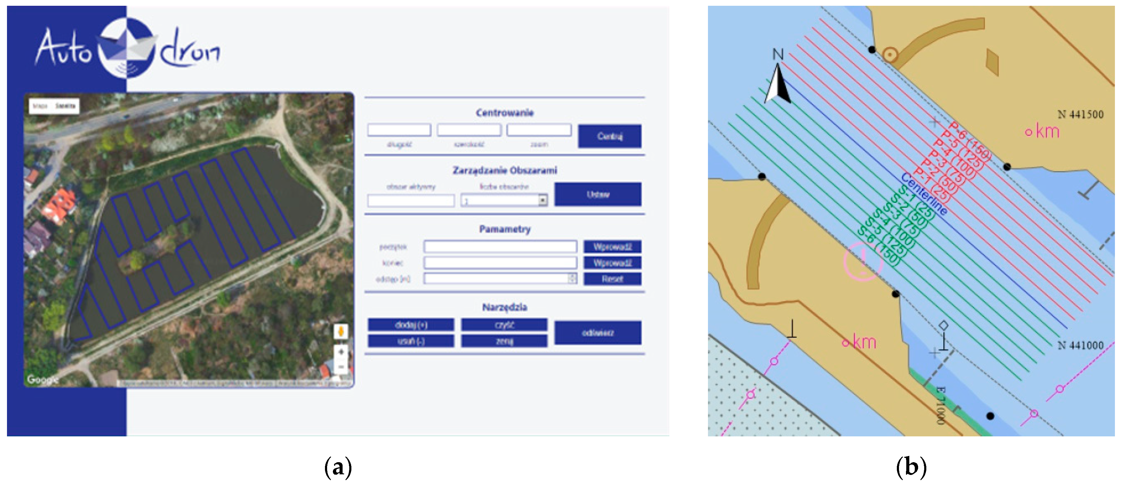
2.2. Planning the Hydrographic Survey to Establish the Territorial Sea Baseline
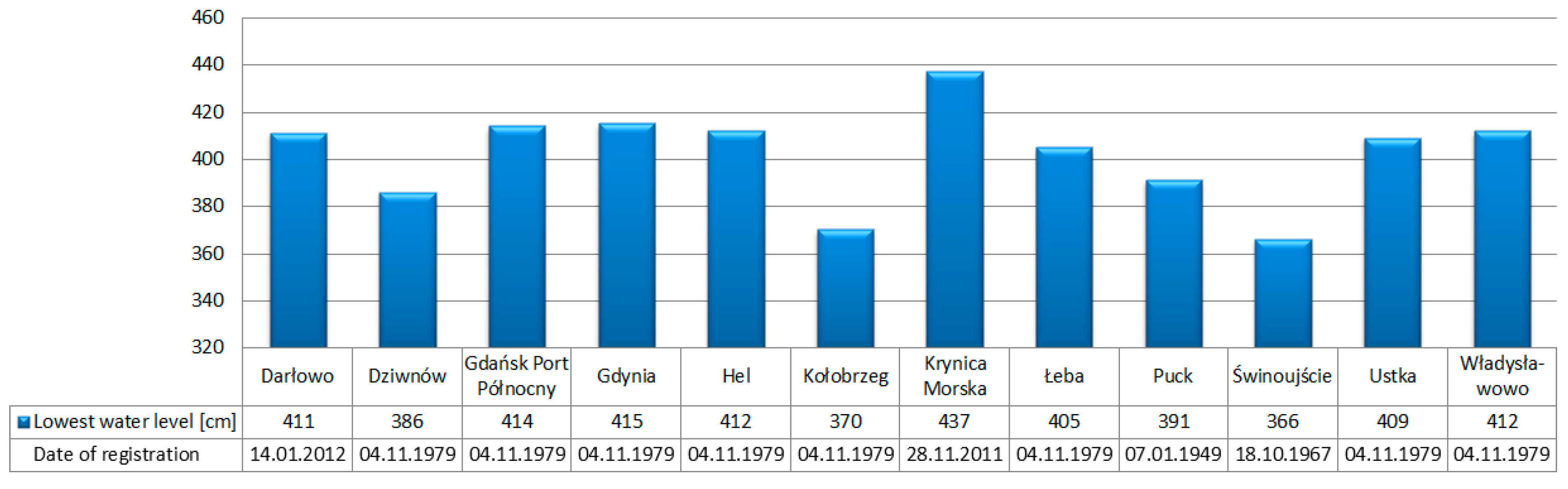
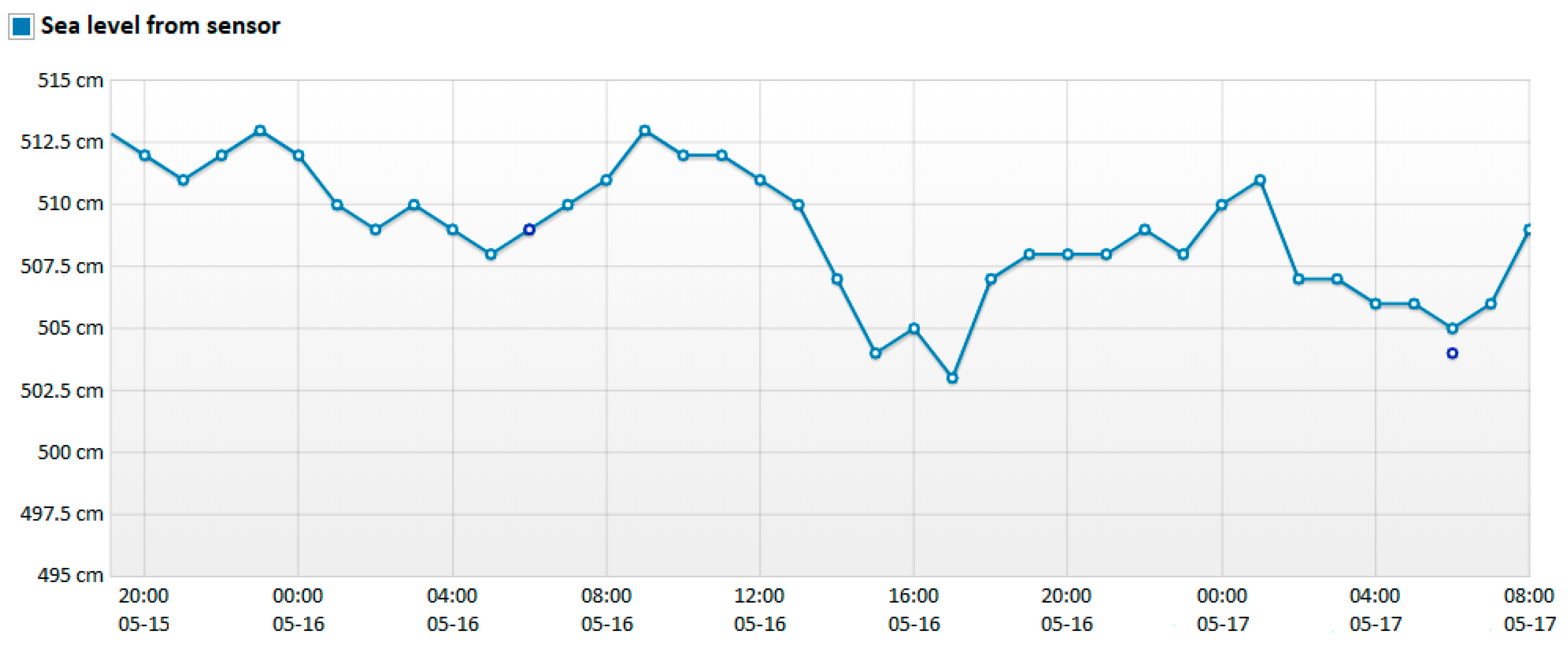
3. Water Level Measurement
- HCWL is the current water level in the adopted reference frame [m],
- HLW is the lowest water level in the adopted reference frame [m].
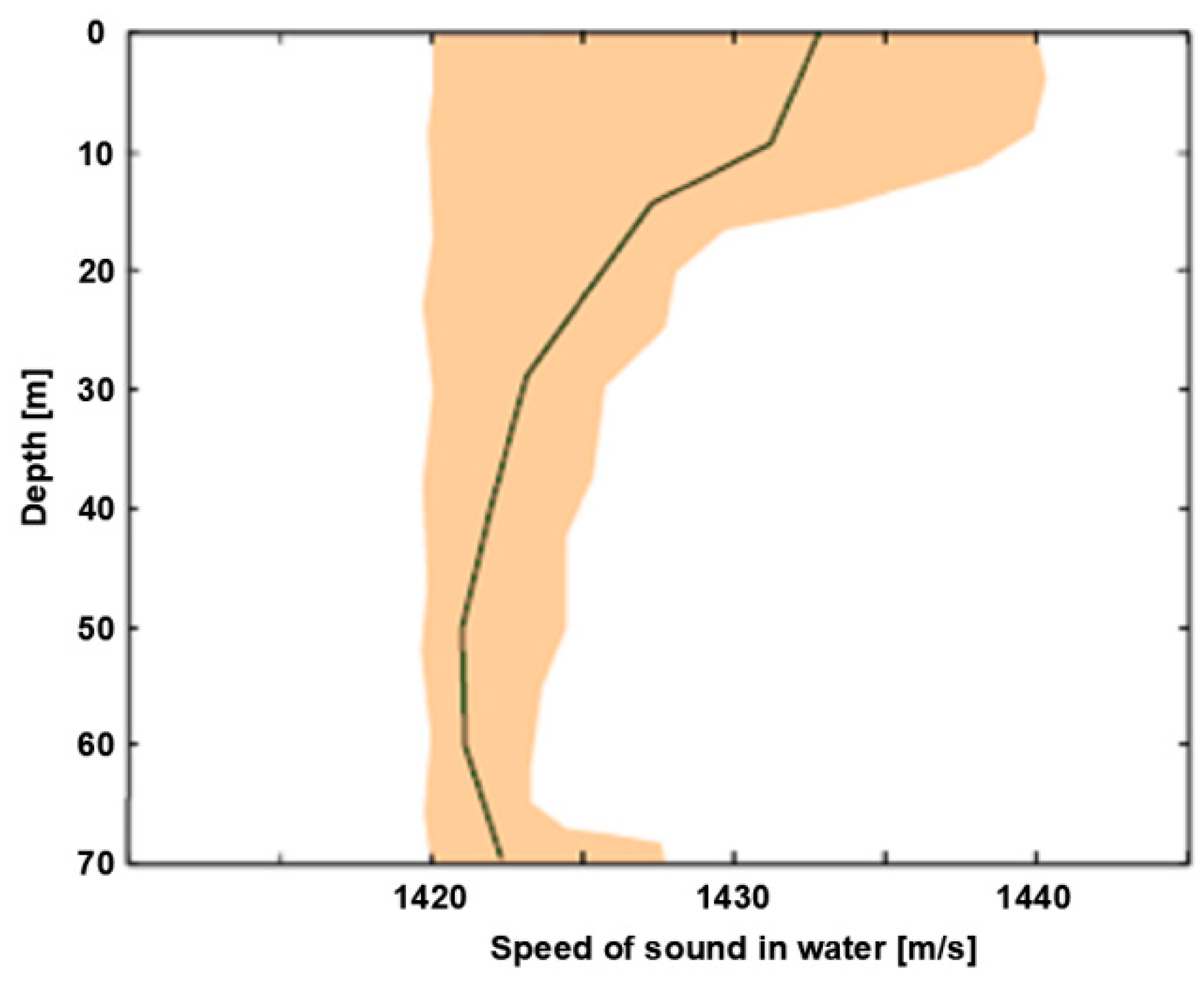
4. Other Oceanographic Measurements
5. Hydrographic Depth Measurement
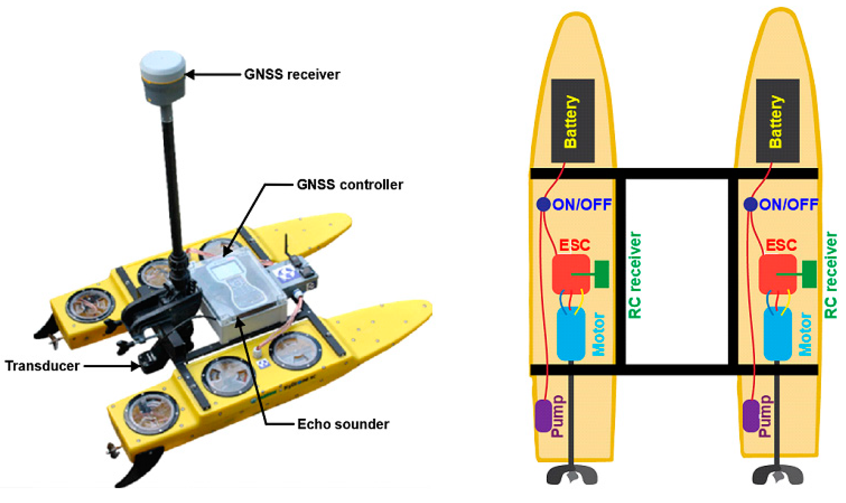
- a miniature SBES
- a GNSS receiver using a GNSS geodetic network or a DGPS receiver.
- measurement of the vertical distribution of the speed of sound in water
- measurement of the draft of the echo sounder transducer.
- a GNSS receiver using a GNSS geodetic network
- a DGPS receiver.
6. Discussions
Author Contributions
Funding
Conflicts of Interest
References
- Klein, N. Litigating International Law Disputes: Weighing the Options; Cambridge University Press: New York, NY, USA, 2014. [Google Scholar]
- Pina-Garcia, F.; Pereda-Garcia, R.; de Luis-Ruiz, J.M.; Perez-Alvarez, R.; Husillos-Rodriguez, R. Determination of Geometry and Measurement of Maritime-Terrestrial Lines by Means of Fractals: Application to the Coast of Cantabria (Spain). J. Coast. Res. 2016, 32, 1174–1183. [Google Scholar] [CrossRef]
- Abidin, H.Z.; Sutisna, S.; Padmasari, T.; Villanueva, K.J.; Kahar, J. Geodetic Datum of Indonesian Maritime Boundaries: Status and Problems. Mar. Geod. 2005, 28, 291–304. [Google Scholar] [CrossRef]
- Horemuz, M. Error Calculation in Maritime Delimitation between States with Opposite or Adjacent Coasts. Mar. Geod. 1999, 22, 1–17. [Google Scholar] [CrossRef]
- UNCLOS. United Nations Convention on the Law of the Sea of 10 December 1982; UNCLOS: Montego Bay, Jamaica, 1982. [Google Scholar]
- Council of Ministers of the Republic of Poland. Ordinance of the Council of Ministers of 13 January 2017 on the Detailed Course of the Baseline, External Boundary of the Territorial Sea and the External Boundary of Contiguous Zone of the Republic of Poland; Council of Ministers of the Republic of Poland: Warsaw, Poland, 2017. (In Polish)
- Ministry of Infrastructure and Development of the Republic of Poland. Justification of the Draft Ordinance of the Council of Ministers on the Detailed Course of the Baseline, External Boundary of the Territorial Sea and the External Boundary of Contiguous Zone of the Republic of Poland. Available online: https://www.senat.gov.pl/download/gfx/senat/pl/senatposiedzeniatematy/2737/drukisejmowe/3661.pdf (accessed on 5 July 2019). (In Polish)
- Specht, C.; Weintrit, A.; Specht, M.; Dąbrowski, P. Determination of the Territorial Sea Baseline—Measurement Aspect. IOP Conf. Ser.Earth Environ. Sci. 2017, 95, 1–10. [Google Scholar] [CrossRef]
- IHO. IHO Standards for Hydrographic Surveys, Special Publication No. 44, 5th ed.; International Hydrographic Organization: Monaco, 2008. [Google Scholar]
- Specht, C.; Weintrit, A.; Specht, M. Determination of the Territorial Sea Baseline—Aspect of Using Unmanned Hydrographic Vessels. TransNav 2016, 10, 649–654. [Google Scholar] [CrossRef]
- Specht, C.; Specht, M.; Cywiński, P.; Skóra, M.; Marchel, Ł.; Szychowski, P. A New Method for Determining the Territorial Sea Baseline Using an Unmanned, Hydrographic Surface Vessel. J. Coast. Res. 2019, 35, 925–936. [Google Scholar] [CrossRef]
- Boon, M.A.; Greenfield, R.; Tesfamichael, S. Wetland Assessment Using Unmanned Aerial Vehicle (UAV) Photogrammetry. Int. Arch. Photogramm. Remote Sens. Spat. Inf. Sci. 2016, XLI-B1, 781–788. [Google Scholar] [CrossRef]
- Lin, Y.; Hyyppa, J.; Jaakkola, A. Mini-UAV-Borne LIDAR for Fine-Scale Mapping. IEEE Geosci. Remote Sens. Lett. 2011, 8, 426–430. [Google Scholar] [CrossRef]
- Grządziel, A.; Wąż, M. Estimation of Effective Swath Width for Dual-Head Multibeam Echosounder. Annu. Navig. 2016, 23, 173–183. [Google Scholar] [CrossRef]
- Lucieer, V.; Huang, Z.; Siwabessy, J. Analyzing Uncertainty in Multibeam Bathymetric Data and the Impact on Derived Seafloor Attributes. Mar. Geod. 2016, 39, 32–52. [Google Scholar] [CrossRef]
- NOAA. NOS Hydrographic Surveys Specifications and Deliverables; National Oceanic and Atmospheric Administration: Silver Spring, MD, USA, 2017. [Google Scholar]
- USACE. EM 1110-2-1003 USACE Standards for Hydrographic Surveys; USACE: Washington, DC, USA, 2013.
- Specht, M.; Specht, C. Hydrographic Survey Planning for the Determination of Territorial Sea Baseline on the Example of Selected Polish Sea Areas. In Proceedings of the 18th International Multidisciplinary Scientific GeoConference (SGEM 2018), Albena, Bulgaria, 30 June–9 July 2018. [Google Scholar] [CrossRef]
- Specht, C.; Świtalski, E.; Specht, M. Application of an Autonomous/Unmanned Survey Vessel (ASV/USV) in Bathymetric Measurements. Pol. Marit. Res. 2017, 24, 36–44. [Google Scholar] [CrossRef]
- Calderbank, B.; MacLeod, A.M.; McDorman, T.L.; Gray, D.H. Canada’s Offshore: Jurisdiction, Rights and Management; Trafford Publishing: Victoria, BC, Canada, 2006. [Google Scholar]
- Kurałowicz, Z.; Słomska, A. Surfaces and Vertical Reference Systems—Observations at Mareograph Stations in Kronstadt and Amsterdam. Mar. Eng. Geotech. 2014, 5, 377–384. (In Polish) [Google Scholar]
- Council of Ministers of the Republic of Poland. Ordinance of the Council of Ministers of 15 October 2012 on the National Spatial Reference System; Council of Ministers of the Republic of Poland: Warsaw, Poland, 2012. (In Polish)
- Medvedev, I.P.; Rabinovich, A.B.; Kulikov, E.A. Tidal Oscillations in the Baltic Sea. Oceanology 2013, 53, 526–538. [Google Scholar] [CrossRef]
- UKHO. ADMIRALTY Tide Tables; UKHO: Taunton, UK, 2019.
- Talley, L.D.; Pickard, G.L.; Emery, W.J.; Swift, J.H. Descriptive Physical Oceanography: An Introduction; Academic Press: Amsterdam-Boston, MA, USA, 2011. [Google Scholar]
- Makar, A. Method of Determination of Acoustic Wave Reflection Points in Geodesic Bathymetric Surveys. Annu. Navig. 2008, 14, 1–89. [Google Scholar]
- Wilson, W.D. Extrapolation of the Equation for the Speed of Sound in Sea Water. J. Acoust. Soc. Am. 1962, 34, 866. [Google Scholar] [CrossRef]
- Woźniak, B.; Bradtke, K.; Derecki, M.; Dera, M.; Dudzińska-Nowak, J.; Dzierzbicka-Głowacka, L.; Ficek, D.; Furmańczyk, K.; Kowalewski, M.; Krężel, A.; et al. SatBałtyk—A Baltic Environmental Satellite Remote Sensing System—An Ongoing Project in Poland. Part 1: Assumptions, Scope and Operating Range. Oceanologia 2011, 53, 897–924. [Google Scholar] [CrossRef]
- Woźniak, B.; Bradtke, K.; Derecki, M.; Dera, M.; Dudzińska-Nowak, J.; Dzierzbicka-Głowacka, L.; Ficek, D.; Furmańczyk, K.; Kowalewski, M.; Krężel, A.; et al. SatBałtyk—A Baltic Environmental Satellite Remote Sensing System—An Ongoing Project in Poland. Part 2: Practical Applicability and Preliminary Results. Oceanologia 2011, 53, 925–958. [Google Scholar] [CrossRef]
- Ostrowska, M.; Darecki, M.; Krężel, A.; Ficek, D.; Furmańczyk, K. Practical Applicability and Preliminary Results of the Baltic Environmental Satellite Remote Sensing System (Satbałtyk). Pol. Marit. Res. 2015, 22, 43–49. [Google Scholar] [CrossRef]
- Giordano, F.; Mattei, G.; Parente, C.; Peluso, F.; Santamaria, R. Integrating Sensors into a Marine Drone for Bathymetric 3D Surveys in Shallow Waters. Sensors 2016, 16, 41. [Google Scholar] [CrossRef]
- Giordano, F.; Mattei, G.; Parente, C.; Peluso, F.; Santamaria, R. MicroVEGA (Micro Vessel for Geodetics Application): A Marine Drone for the Acquisition of Bathymetric Data for GIS Applications. Int. Arch. Photogramm. Remote Sens. Spat. Inf. Sci. 2015, 40, 123–130. [Google Scholar] [CrossRef]
- Liang, J.; Zhang, J.; Ma, Y.; Zhang, C.Y. Derivation of Bathymetry from High-Resolution Optical Satellite Imagery and USV Sounding Data. Mar. Geod. 2017, 40, 466–479. [Google Scholar] [CrossRef]
- Mattei, G.; Troisi, S.; Aucelli, P.P.C.; Pappone, G.; Peluso, F.; Stefanile, M. Sensing the Submerged Landscape of Nisida Roman Harbour in the Gulf of Naples from Integrated Measurements on a USV. Water 2018, 10, 1686. [Google Scholar] [CrossRef]
- Stateczny, A.; Gierski, W. The Concept of Anti-Collision System of Autonomous Surface Vehicle. E3S Web Conf. 2018, 63, 1–6. [Google Scholar] [CrossRef]
- Stateczny, A.; Kazimierski, W.; Burdziakowski, P.; Motyl, W.; Wisniewska, M. Shore Construction Detection by Automotive Radar for the Needs of Autonomous Surface Vehicle Navigation. Int. J. Geo-Inf. 2019, 8, 80. [Google Scholar] [CrossRef]
- Demer, D.A.; Berger, L.; Bernasconi, M.; Bethke, E.; Boswell, K.; Chu, D.; Domokos, R.; Dunford, A.; Fässler, S.; Gauthier, S.; et al. Calibration of Acoustic Instruments, ICES Cooperative Research Report; International Council for the Exploration of the Sea: Copenhagen, Denmark, 2015. [Google Scholar]
- Grządziel, A.; Felski, A.; Wąż, M. Experience with the Use of a Rigidly-Mounted Side-Scan Sonar in a Harbour Basin Bottom Investigation. Ocean. Eng. 2015, 109, 439–443. [Google Scholar]
- Iwen, D. Horizontal Accuracy Issues During MBES Surveys. Annu. Navig. 2017, 24, 67–73. [Google Scholar] [CrossRef]
- Makar, A. Dynamic Tests of ASG-EUPOS Receiver in Hydrographic Application. In Proceedings of the 18th International Multidisciplinary Scientific GeoConference (SGEM 2018), Albena, Bulgaria, 30 June–9 July 2018. [Google Scholar]
- Rogowski, J.; Specht, C.; Weintrit, A.; Leszczyński, W. Evaluation of Positioning Functionality in ASG EUPOS for Hydrography and Off-Shore Navigation. TransNav 2015, 9, 221–227. [Google Scholar] [CrossRef]
- Specht, C.; Makar, A.; Specht, M. Availability of the GNSS Geodetic Networks Position During the Hydrographic Surveys in the Ports. TransNav 2018, 12, 657–661. [Google Scholar] [CrossRef]
- Specht, C.; Specht, M.; Dąbrowski, P. Comparative Analysis of Active Geodetic Networks in Poland. In Proceedings of the 17th International Multidisciplinary Scientific GeoConference (SGEM 2017), Albena, Bulgaria, 27 June–6 July 2017. [Google Scholar] [CrossRef]
- Specht, M.; Specht, C. The Use of GNSS Geodetic Networks on the Approach to the Ports—Gulf of Gdańsk Study. In Proceedings of the 18th International Multidisciplinary Scientific GeoConference (SGEM 2018), Albena, Bulgaria, 30 June–9 July 2018. [Google Scholar] [CrossRef]
- Lubis, M.Z.; Anggraini, K.; Kausarian, H.; Pujiyati, S. Review: Marine Seismic and Side-Scan Sonar Investigations for Seabed Identification with Sonar System. J. Geosci. Eng. Environ. Technol. 2017, 2, 166–170. [Google Scholar] [CrossRef]
- Ratheesh, R.; Ritesh, A.; Remya, P.G.; Nagakumar, K.C.V.; Demudu, G.; Rajawat, A.S.; Nair, B.; Nageswara Rao, K. Modelling Coastal Erosion: A Case Study of Yarada Beach Near Visakhapatnam, East Coast of India. Ocean Coast. Manag. 2018, 156, 239–248. [Google Scholar]
- Specht, C.; Pawelski, J.; Smolarek, L.; Specht, M.; Dąbrowski, P. Assessment of the Positioning Accuracy of DGPS and EGNOS Systems in the Bay of Gdansk Using Maritime Dynamic Measurements. J. Navig. 2019, 72, 575–587. [Google Scholar] [CrossRef]
- Ward, R.D.; Burnside, N.G.; Joyce, C.B.; Sepp, K.; Teasdale, P.A. Improved Modelling of the Impacts of Sea Level Rise on Coastal Wetland Plant Communities. Hydrobiologia 2016, 774, 203–216. [Google Scholar] [CrossRef]
- IALA. IALA Recommendation R-121 on the Performance and Monitoring of DGNSS Services in the Frequency Band 283.5–325 kHz, 1.1 ed.; IALA: Saint-Germain-en-Laye, France, 2004. [Google Scholar]
- Kim, J.; Song, J.; No, H.; Han, D.; Kim, D.; Park, B.; Kee, C. Accuracy Improvement of DGPS for Low-Cost Single-Frequency Receiver Using Modified Flachen Korrektur Parameter Correction. Int. J. Geo-Inf. 2017, 6, 222. [Google Scholar] [CrossRef]


| Order | Special | 1a | 1b | 2 |
|---|---|---|---|---|
| Description of areas | Areas where under-keel clearance is critical | Areas shallower than 100 m where under-keel clearance is less critical but features of concern to surface shipping may exist | Areas shallower than 100 m where under-keel clearance is not considered to be an issue for the type of surface shipping expected to transit the area | Areas generally deeper than 100 m where a general description of the seafloor is considered adequate |
| Full seafloor search | Required | Required | Not required | Not required |
| Recommended maximum line spacing | Not defined as full seafloor search is required | Not defined as full seafloor search is required | 3× average depth or 25 m, whichever is greater | 4× average depth |
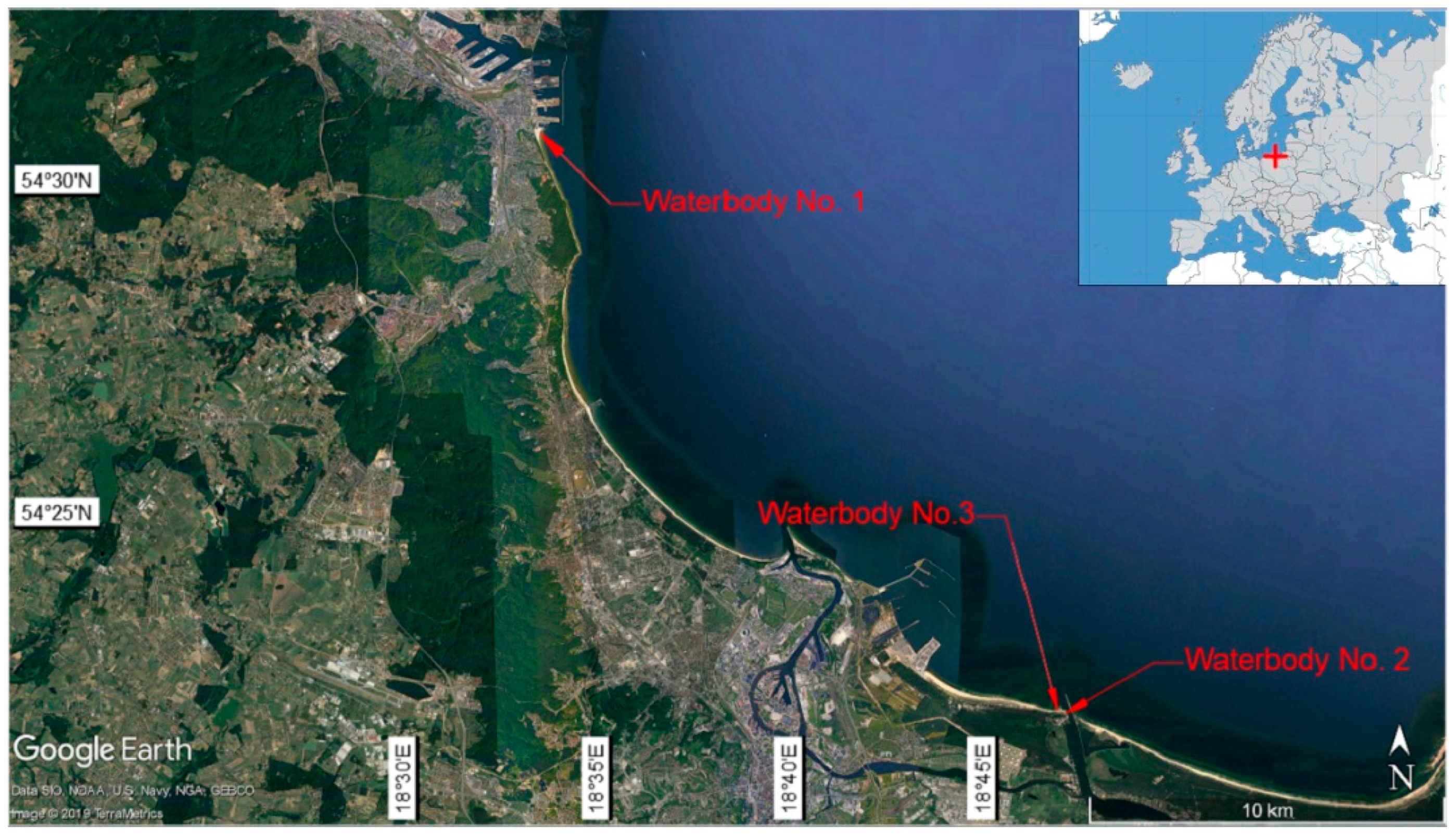
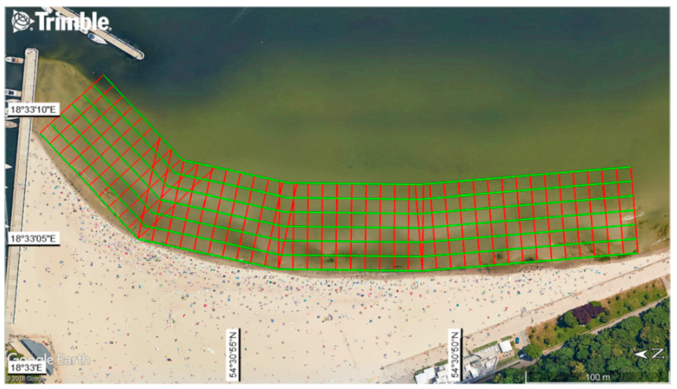
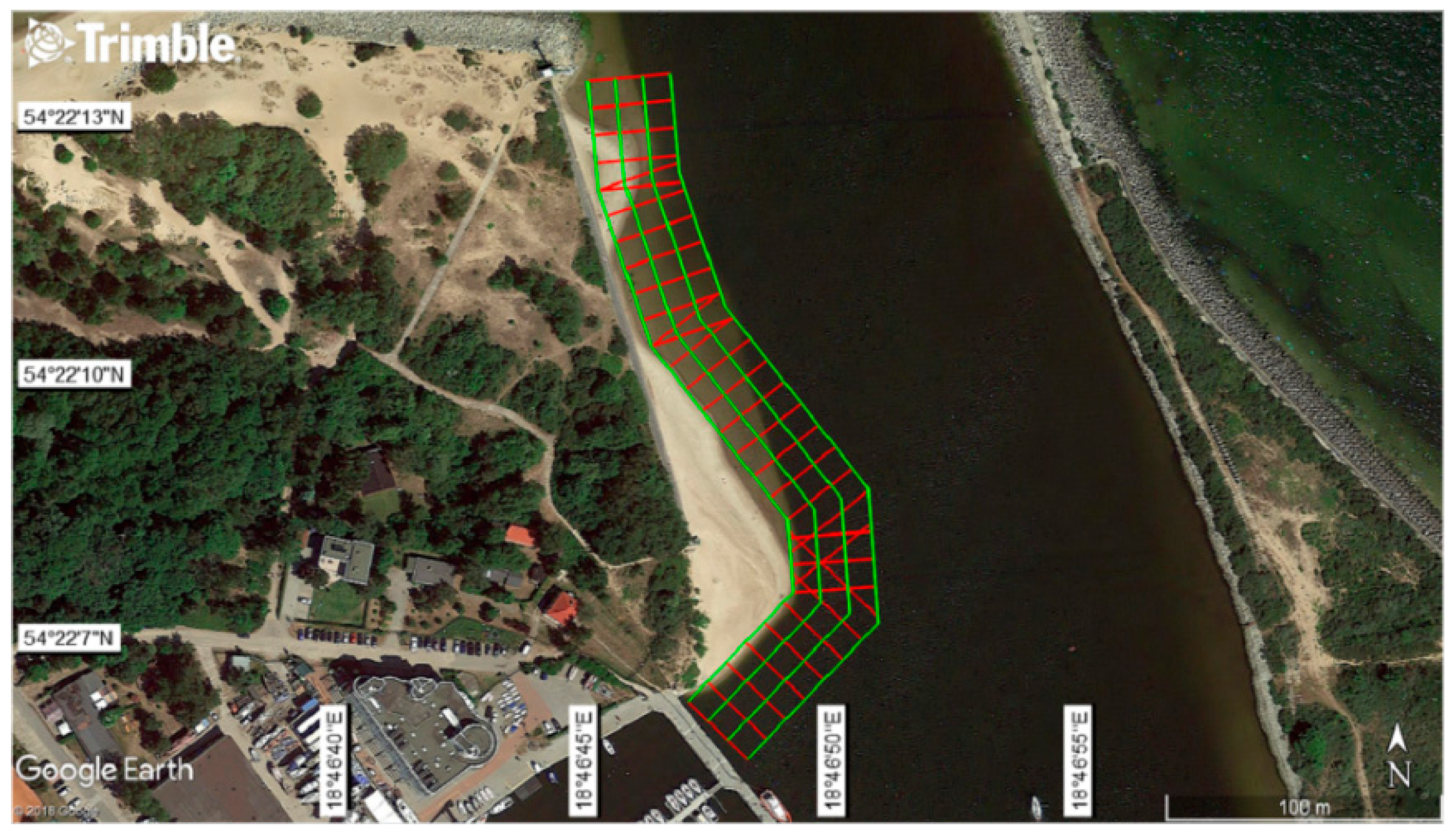
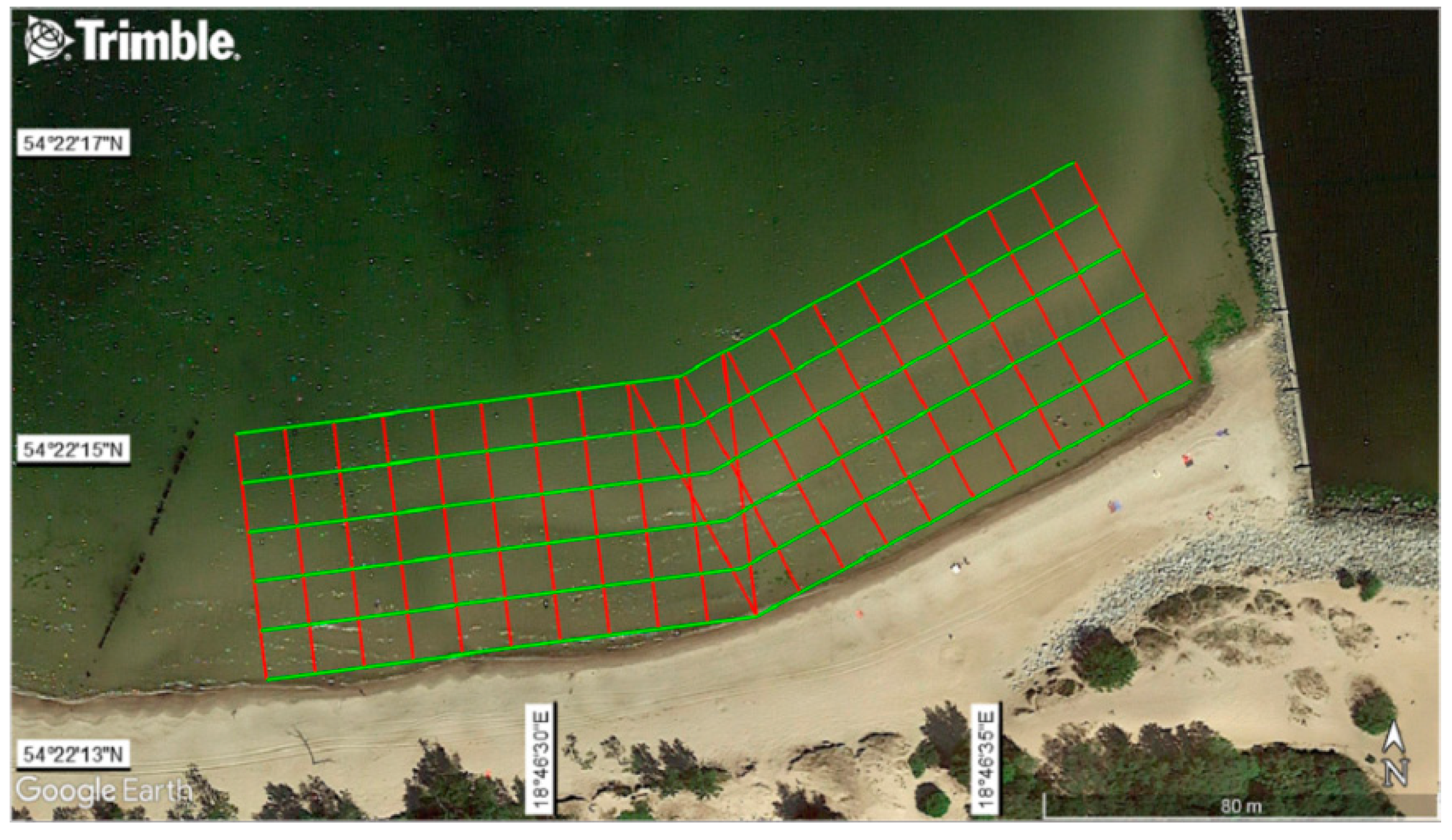
| Name of Waterbody | Features | Photograph |
|---|---|---|
| Waterbody No. 1: Open sea public beach in Gdynia | A typical coastline (straight line sandy section), reinforced with tetrapods and concrete wharfs. The length of the waterbody along the coastline is about 450 m. |  |
| Waterbody No. 2: River mouth the Vistula river mouth near the National Sailing Centre in Gdańsk | A waterbody of great dynamics of hydromorphological features. It is a natural area (with no hydrotechnical structures). The length of the waterbody along the coastline is about 250 m. |  |
| Waterbody No. 3: Exit from a large port area near the entrance to the Górki Zachodnie from Bay of Gdańsk | A waterbody with a large number of hydrotechnical structures. The length of the waterbody along the coastline is about 250 m. |  |
© 2019 by the authors. Licensee MDPI, Basel, Switzerland. This article is an open access article distributed under the terms and conditions of the Creative Commons Attribution (CC BY) license (http://creativecommons.org/licenses/by/4.0/).
Share and Cite
Specht, M.; Specht, C.; Wąż, M.; Naus, K.; Grządziel, A.; Iwen, D. Methodology for Performing Territorial Sea Baseline Measurements in Selected Waterbodies of Poland. Appl. Sci. 2019, 9, 3053. https://doi.org/10.3390/app9153053
Specht M, Specht C, Wąż M, Naus K, Grządziel A, Iwen D. Methodology for Performing Territorial Sea Baseline Measurements in Selected Waterbodies of Poland. Applied Sciences. 2019; 9(15):3053. https://doi.org/10.3390/app9153053
Chicago/Turabian StyleSpecht, Mariusz, Cezary Specht, Mariusz Wąż, Krzysztof Naus, Artur Grządziel, and Dominik Iwen. 2019. "Methodology for Performing Territorial Sea Baseline Measurements in Selected Waterbodies of Poland" Applied Sciences 9, no. 15: 3053. https://doi.org/10.3390/app9153053
APA StyleSpecht, M., Specht, C., Wąż, M., Naus, K., Grządziel, A., & Iwen, D. (2019). Methodology for Performing Territorial Sea Baseline Measurements in Selected Waterbodies of Poland. Applied Sciences, 9(15), 3053. https://doi.org/10.3390/app9153053