VS-GRU: A Variable Sensitive Gated Recurrent Neural Network for Multivariate Time Series with Massive Missing Values

Abstract

Multivariate time series are often accompanied with missing values, especially in clinical time series, which usually contain more than 80% of missing data, and the missing rates between different variables vary widely. However, few studies address these missing rate differences and extract univariate missing patterns simultaneously before mixing them in the model training procedure. In this paper, we propose a novel recurrent neural network called variable sensitive GRU (VS-GRU), which utilizes the different missing rate of each variable as another input and learns the feature of different variables separately, reducing the harmful impact of variables with high missing rates. Experiments show that VS-GRU outperforms the state-of-the-art method in two real-world clinical datasets (MIMIC-III, PhysioNet).

1. Introduction

Studies on Electronic Health Records (EHRs) [1] play an important role in modern society [2]. According to the International Organization for Standardization (ISO) definition [3], EHRs mean a repository of patient data in digital form, which includes diagnostic records, electronic medical images, patient history, allergies and laboratory test results, etc. Healthcare workers rely on EHRs to bill patients and evaluate the physical conditions of patients [4]. In addition, more and more studies focus on using machine learning to deal with EHRs for the large amount of data. In this paper, we study the clinical time series, which originates from sensors in intensive care units (ICUs) or is recorded manually. Under most circumstances, these records are multivariate, including heart rate, blood pressure, and weight, etc. Generally, researchers analyze the multivariate time series of EHRs to accomplish the following tasks: in-hospital morality classification [5], diagnosis classification [6] and length of stay classification problems [7]. Because it is unnecessary to record all variables at all times, resulting in massive missing values, one of the major challenges of clinical time series classification tasks is to deal with the massive missing data. Figure 1 shows an example of a clinical time series. It should be noted that the observation frequency is usually quite different between different variables.

Traditionally, in order to do the classification task on clinical time series, we will impute the missing values in the time series first. After imputing the missing data or simply omitting it [8], we feed the processed data to the auto-regressive integrated moving average (ARIMA) model [9] and the Kalman filter [10], treating it as a normal time series classification problem [11,12,13]. Most people impute missing values with the mean value in the training set (mean imputation) or the last observation (forward imputation) for effectiveness and efficiency [14]. We can apply not only the simple methods mentioned above but also various advanced methods, such as matrix factorization [15], kernel methods [16], and the EM algorithm [17], to perform the imputation. However, missing data imputation only serves as an auxiliary function to improve classification accuracy, and some advanced methods may cause time-consuming and expensive computational problems without classification performance improvement. Moreover, many imputation methods may fail in dealing with such massive missing values [18]. Thus, the solutions of time series with no or few missing values and time series with massive missing values in classification tasks should be different.

When most of the multivariate time series is missing, we need to find more features besides the time series itself. The missing values in clinical time series are caused by many reasons. The most important one is that it costs much money and time to ask healthcare workers to record every possible variable of the patients [19]. Usually, they only choose to record the variables related to the medical condition of the patients. For example, heart rate may be recorded more frequently when the patients have heart disease. In addition, when the condition of the patients get worse, the recording frequency becomes higher. Finally, automated monitoring devices might fail to record the variables sometimes, but it is rarer than the previous cases we discuss above. We define the information contained in whether to record the variable (missing mark) and how often to record it (missing rate) as a missing pattern of a variable in the multivariate clinical time series. Take the patients with heart disease as examples: we believe the missing pattern of variables related to heart conditions behaves differently from others. Moreover, we should process the missing patterns of different variables separately to fully exploit the information from the multivariate time series.

With the development of deep learning, recurrent neural networks (RNN) have become one of the most widely used models to solve time series problems for the reason that they can directly handle time series of varying length [20]. Long short-term memory (LSTM) and gated recurrent units (GRU) are the most popular RNN models for capturing long-term and short-term impacts in time series [21,22]. Even though few studies focus on handling multivariate time series with massive missing data, there are still some outstanding works that have been proposed recently. GRU-D proposed by Che et al. [23] focuses on the missing pattern of multivariate time series. However, GRU-D treats multivariate time series as a whole and it does not consider the missing rate differences. Harutyunyan et al. separate the multivariate time series into univariate time series and use an independent LSTM network for every variable to fully extract the single variable feature and its missing pattern at the cost of time consumption [24].

In this paper, we propose our method called variable sensitive GRU (VS-GRU), which has the following contributions:

• In clinical time series, we believe the missing rate of variable is related to its characteristic. In addition to the missing mark, VS-GRU considers the missing rate of different variables, seeing it as another input of GRU.
• VS-GRU processes variables separately at the same time in a simple structure. Variables can maintain its characteristics before being mixed with others, which increases robustness when dealing with time series with some variables that are almost completely missing.
• VS-GRU considers the classification result at every time step, which decreases the probability of learning error from the whole time series.

In Section 2, we present the related recent research in time series with missing values’ classification problems and clinical time series analyses using deep learning. In Section 3, VS-GRU is presented in detail. We evaluate our method on two public clinical datasets and compare it with the state-of-the-art in Section 4. Finally, we make our conclusions in Section 5.

2. Related Works

2.1. Time Series with the Missing Values Classification Problem

A considerable amount of literature has been published on time series with missing values. Many of these works focus on the imputation of missing values [15,25]. The classification problem can be solved after the imputation procedure using traditional classification methods such as kernel method [26], support vector machines [27] and random forest [12]. However, most of the traditional methods can not directly handle multivariate time series of varying length. Futoma et al. used multi-task Gaussian processes to directly transform the irregular sampled time series with missing values into a more uniform representation and then do the classification task [28]. Recently, Mikalsen et al. proposed a kernel method called time series cluster kernel (TCK) [29] to learn the similarities between multivariate time series. It can directly handle time series of varying lengths and with missing data without an imputation method. However, the maximum missing rate shown in this research is 50%, which is not enough to deal with massive missing values in clinical time series and TCK assumes that missing values in time series occur at random. Later, they proposed an improved kernel to exploit the informative missingness when the missing values occur non-randomly [30].

Besides kernel methods, researchers also choose RNN to address the missing values problem in time series. Yoon et al. indicated that the information within variables is as important as the information across variables in the procedure of imputation [31]. They used multi-directional recurrent neural networks with interpolation blocks and imputation block to impute the missing values. Lipton et al. considered the missing mark very important. They concatenated the missing mark and the time series and input them into LSTM [13]. They used the forward or backward imputation methods to address missing values. If the variable in a time series is completely missing, it will be filled with expert experience values. Later, Lipton et al. proposed an improved method [18], which is added to the mean value, standard deviation, and the first and the last observation of each variable in a multivariate time series into the model. These added features characterize the difference of each variable, but they are calculated manually and remain the same during the training process. Che et al. changed the framework of GRU and treated the missing mark as another input and fed both missing mark and time series into a GRU model, called GRU-D [23]. Harutyunyan et al. proposed channel-wise LSTM [24]. They input a single variable along with its missing mark into an independent bidirectional LSTM layer and then concatenated all the outputs and fed them into the same LSTM layer. Thus, the information related to univariable can be learned before the variables are mixed in LSTM. However, because each variable needs to be trained in an independent network, it causes intensive computations.

2.2. Clinical Time Series Analysis Using Deep Learning

In the clinical field, scoring methods to evaluate the condition of patients such as SAPS-II [32], SOFA [33] and APACHE [34] have already been used in practice. Most of these scoring methods use simple models, such as logistic regression, to perform the classification task, and the data for training are selected manually. However, the accuracy of these methods has been doubted by earlier studies [35,36]. With the development of deep learning, researchers have tried to replace these simple models with deep learning models to handle clinical time series problems.

There are two main problems in clinical time series: missing values and irregular sampling rate. To deal with missing values, the first systematic study of clinical time series problem based on RNN was reported by Lipton et al. in 2016. Choi et al. used RNN to perform a different diagnosis on clinical data with diagnosis codes, medication codes and procedure codes, and they called it doctor AI [6]. Strauman et al. simply applied GRU-D to detect surgical site infection and added a weighting scheme in calculating loss due to the class imbalance in clinical data [37]. Purushotham et al. proposed ensemble learning methods to combine GRU and forward neural networks, which is called the multi-modal deep learning model (MMDL) to simultaneously learn the time-variant information and nontime-variant information [38]. In the aspect of dealing with irregular sampling rate, Che et al. proposed a deep generative model to capture temporal dependencies in multi-rate multivariate time series [39]. Bahadori et al. used an augmentation technique to merge the record more closely-spaced in time at first and put the processed data into a neural network classifiers [40]. Shukla et al. chose to deal with missing values and irregular sampling rate problems at the same time. They introduced a two-layer interpolation network to interpolate multivariate time series. The first layer performs univariate transformations separately and the second layer merges information across all dimensions [41].

Our method is designed to handle multivariate time series with massive missing values. It can directly process time series without considering a two-step procedure. The manually calculated features of different variables are not required because it can explore the feature of different variables at the same time automatically without additional computing cost.

3. Methods

3.1. Notation

We define a multivariate time series of length T and D as $x={\left\{x_1,x_2,\dots ,x_T\right\}}^T\in {\mathbb{R}}^{T\times D}$, in which $x_t^d,t\in \left\{1,2,\dots ,T\right\},d\in \left\{1,2,\dots ,D\right\}$ indicates that the observation of variable d at the time of $s_t$. To distinguish the difference between the real observation and the imputed value, we introduce a mask indicator $m={\left\{m_1,m_2,\dots ,m_T\right\}}^T\in {\mathbb{R}}^{T\times D}$, which determines at time step t whether there is an observation of variable d:

$$m_t^d=\left\{\begin{array}{cc}1,\hfill & \mathrm{if}{x}_t^d\mathrm{is}\mathrm{observed},\hfill \\ 0,\hfill & \mathrm{otherwise}.\hfill \end{array}\right.$$

(1)

In addition, we calculate the missing rate $\mu$ of each variable d in each time series x of length T:

$${\mu }^d=1-\frac{1}{T}\sum _{t=1}^T{m}_t^d.$$

(2)

For a time series x, we record the time interval between the imputed values at time step t and the last observation of variable d, which is $\delta ={\left\{{\delta }_1,{\delta }_2,\dots ,{\delta }_T\right\}}^T\in {\mathbb{R}}^{T\times D}$,

$${\delta }_t^d=\left\{\begin{array}{cc}{s}_t-s_{t-1}+{\delta }_{t-1}^d,\hfill & t>1,m_{t-1}^d=0,\hfill \\ s_t-s_{t-1},\hfill & t>1,m_{t-1}^d=1,\hfill \\ 0,\hfill & t=1.\hfill \end{array}\right.$$

(3)

$s_t$ denotes the time that observation is recorded.

3.2. GRU

To address the gradient explosion and gradient vanishing problems in RNN, GRU applies the reset gate and update gate to control how the information from the past and current input change the current state simultaneously.

Figure 2 shows the GRU structure. At time step t, GRU receives the input $x_t$ and updates the hidden state $h_t$. The reset gate $r_t$ takes input $x_t$ and calculates the candidate hidden state ${\tilde{h}}_t$. Update gate $z_t$ chooses information from the current candidate hidden state ${\tilde{h}}_t$ and the last time step hidden state $h_{t-1}$ and outputs $h_t$. The update functions are as follows:

$$z_t=\sigma \left(W_z{x}_t+U_z{h}_{t-1}+b_z\right),$$

(4)

$$r_t=\sigma \left(W_r{x}_t+U_r{h}_{t-1}+b_r\right),$$

(5)

$${\tilde{h}}_t=tanh\left(W_h{x}_t+U_h\left(r_t\odot h_{t-1}\right)+b_h\right),$$

(6)

$$h_t=\left(1-z_t\right)\odot h_{t-1}+z_t\odot {\tilde{h}}_t.$$

(7)

⊙ indicates element-wise multiplication.

3.3. GRU-D

GRU-D is an improved version of GRU for time series with missing values. It introduces a decay mechanism to the input time series x and hidden state $h_t$, which will be adopted in our method. The imputed values of variable d decay from the last observation to the average value; that is, the longer between the imputed values from the last real observation, the closer it is to the average value. We regard it as a dynamic imputation mechanism that is shown in Equation (8) in detail. In Equation (8), $x_{t^{\prime }}^{\mathrm{d}}$ indicates the last observation of variable d and ${\tilde{x}}^d$ indicates the mean of variable d in the training set:

$${\widehat{x}}_t^d=m_t^d{x}_t^{\mathrm{d}}+\left(1-m_t^d\right)\left({\gamma }_{x_t}^{\mathrm{d}}{x}_{t^{\prime }}^{\mathrm{d}}+\left(1-{\gamma }_{x_t}^{\mathrm{d}}\right){\tilde{x}}^d\right).$$

(8)

At the same time, hidden state $h_t$ decays from the previous hidden state to zero if time series x contains missing values:

$${\widehat{h}}_{t-1}={\gamma }_{h_t}\odot h_{t-1}.$$

(9)

The decay factor $\gamma$, which is between 0 and 1, is learned while training the model. To clarify, $W_{{\gamma }_x}$ is a diagonal matrix, while $W_{{\gamma }_h}$ is not:

$$\gamma =exp\left\{-max\left(0,W_{\gamma }\delta +b_{\gamma }\right)\right\}.$$

(10)

Moreover, GRU-D directly adds mask indicator m into the reset gate, update gate and candidate hidden state as another input in addition to time series x.

3.4. VS-GRU: Variable Sensitive GRU

3.4.1. Missing Rate Impact

In real life, different variables usually have different monitoring frequencies based on their characteristics. Specifically, in the health care field, the doctor decides which variable needs to be monitored according to the patient’s physical condition. Therefore, it is very common to have variable $d_i$ completely missing while variable $d_j$ fully recorded in a clinical time series. It is a convincing conclusion that the missing rate of the variable is related to its characteristics. Therefore, we should consider the impact of the missing rate of different variables in multivariate time series.

The time interval $\delta$ between current time step and last observation used in the dynamic imputation mechanism implies the missing rate difference to some extent. Usually, a variable with a high missing rate has a larger time interval $\delta$ than others in all time steps. However, it only contains the missing situation before the current time step and it is not enough for the model to fully understand the missing situation in all time steps. We should add the missing rate $\mu$ into the GRU update functions so that every time step in GRU can use the information from the whole time series to solve the classification problem. The missing rate directly tells the differences between variables in multivariate time series. On the other hand, there are experiments to prove that the prediction performance using records within 30 h after admission is close to using records within 48 h [23]. Thus, when we use VS-GRU in practice, if we have new observations to come, we can keep the missing rate unchanged or calculate a new missing rate within a new time interval (like 24 h) and update it. By this way, we can execute VS-GRU efficiently on the fly.

Instead of directly adding the missing rate $\mu$ into the GRU update functions, we choose to use the exponential negative rectifier to map the missing rate $\mu$ into missing factor $\beta$ between 0 and 1. Given that the missing rate of clinical time series is above 80%, the missing rate $\mu$ of different variables in one time series may be close to 1 in many circumstances. The decay equation automatically detects the slight differences between the missing rate of different variables and the model can learn better from missing factor $\beta$:

$$\beta =exp\left\{-max\left(0,W_{\beta }·\mu +b_{\beta }\right)\right\}.$$

(11)

It should be noted that the difference between Equation (11) and Equation (10) is $W_{\beta },$ which is a vector instead of a matrix. $W_{\beta }$ and $b_{\beta }$ share the same dimension as $\mu$. We calculate the dot product of $W_{\beta }$ and $\mu$ and then add the bias $b_{\beta }$. Thus, the missing factor $\beta$ of one variable is only related to itself.

3.4.2. Univariate Missing Pattern Extraction

The weight matrices in the update function of standard GRU are not diagonal matrices so that a variety of variable interaction patterns can be learned from the multivariate time series. However, given that most data are missing in clinical time series, this design combines variables with a low missing rate and variables with a high missing rate and it might be harmful for the model to extract the useful information of the real observations. It goes without saying that the real observations are more critical than the imputations. Because they are mixed together, GRU cannot distinguish them well. Although we add the mask indicator m and missing factor $\beta$ into the update functions, after the transformation, GRU cannot recognize which input $x_t^d$ matches its mask indicator $m_t^d$ and missing factor ${\beta }^d$. As a result, the information of time series x and its missing pattern m and missing factor $\beta$ are learned separately.

To fully learn the information of the real observations, we use the weight vector in the update gate, the reset gate and the candidate hidden state update formulas in GRU, and calculate the vector dot product to perform training. It is the same that we change the matrices into diagonal matrices in order to learn the information of each variable itself. Even though there are some variables completely missing because variable features are learned independently, GRU can still exploit useful information from variables with low missing rates. The update functions are as follows:

$$z_t^1=\sigma \left(W_z^1·{\widehat{x}}_t+U_z^1·{\widehat{h}}_{t-1}^1+V_z^1·m_t+P_z^1·{\beta }^1+b_z^1\right),$$

(12)

$$r_t^1=\sigma \left(W_r^1·{\widehat{x}}_t+U_r^1·{\widehat{h}}_{t-1}^1+V_r^1·m_t+P_r^1·{\beta }^1+b_r^1\right),$$

(13)

$${\tilde{h}}_t^1=tanh\left(W_h^1·{\widehat{x}}_t+U_h^1·\left(r_t^1\odot {\widehat{h}}_{t-1}^1\right)+V_h^1·m_t+P_h^1·{\beta }^1+b_h^1\right),$$

(14)

$$h_t^1=\left(1-z_t^1\right)\odot {\widehat{h}}_{t-1}^1+z_t^1\odot {\tilde{h}}_t^1.$$

(15)

In Equations (12)–(14), $W^1$, $U^1$, $V^1$ and $P^1$ are vectors with the same dimension as variables. ${\beta }^1$ belonging to one variable in the same time series remains the same in all time steps. We adopt decay mechanism of GRU-D to decay input $h_t$ and dynamic imputation mechanism to impute $x_t$, but we use the same form in Equation (11) to calculate ${\gamma }_x$ and ${\gamma }_h$. Each input variable has its independent learning procedure, as shown in Figure 3. A fully connected layer with a sigmoid activation function is added at the output of the GRU layer for the classification problem. This layer can integrate all variables and outputs the probability. We call this GRU framework variable sensitive GRU (VS-GRU), which exploits variables with different missing rate independently and is sensitive to variables with low missing rates. On the other hand, we can see from Equations (12)–(14) that VS-GRU uses a weight vector rather than a weight matrix and updates itself through a vector dot product rather than matrix multiplication. Thus, another advantage of this change is that it can be computed much faster than standard GRU using much less parameters even with the addition of $V^1$ and $P^1$. For example, if we use a standard GRU to process multivariate time series with 10 variables and use 64 hidden units, the total number of parameters is 4190. However, VS-GRU with the decay mechanism and dynamic imputation mechanism only has 230 parameters.

However, VS-GRU only relies on the last fully connected layer to perform variable integration and its simple structure may not be enough to address complex problems such as multi-task classification problems. To address this problem, we propose VS-GRU integration (VS-GRU-i), which consists of two layers of GRU. The first GRU layer is VS-GRU, and the second layer GRU integrates the feature learned from the first layer. We add a penalized mechanism at the input of the second GRU layer to detect if one variable is completely missing or there are only a few observed values. The penalized mechanism can be done by performing the element-wise multiplication of the missing factor $\beta$ and $h_t^1$. The missing factor used in the penalized mechanism does not share the same weight as the missing factor used in the first GRU layer:

$$z_t^2=\sigma \left(W_z^2\left({\beta }^2\odot h_t^1\right)+U_z^2{h}_{t-1}^2+b_z^2\right),$$

(16)

$$r_t^2=\sigma \left(W_r^2\left({\beta }^2\odot h_t^1\right)+U_r^2{h}_{t-1}^2+b_r^2\right),$$

(17)

$${\tilde{h}}_t^2=tanh\left(W_h^2\left({\beta }^2\odot h_t^1\right)+U_h^2\left(r_t^2\odot h_{t-1}^2\right)+b_h^2\right),$$

(18)

$$h_t^2=\left(1-z_t^2\right)\odot h_{t-1}^2+z_t^2\odot {\tilde{h}}_t^2.$$

(19)

In Equations (16)–(18), $W^2$ and $U^2$ are both not diagonal matrices. The decay mechanism and dynamic imputation mechanism are not applied in this GRU layer.

3.4.3. Deep Supervision

At every time step t, GRU outputs its hidden state $h_t$. If we only use the output from the last time step, learning error will be carried through the whole time series and corrected at the last. To avoid this situation, we use the output from all time steps as supervision, which is called deep supervision. Obviously, the output from the last time step is more important than the other outputs from previous time steps, so we use a hyper-parameter $\alpha$ to determine the relative importance between them. Two independent fully connected layers are applied on the last time step and all time steps. Thus, the outputs of the last time step ${\tilde{y}}_T$ in the two parts of loss function are different. The framework of VS-GRU-i applying deep supervision is shown in Figure 4:

$$loss=(1-\alpha )·\frac{1}{T}\sum _{t=1}^T{loss}_t\left({\tilde{y}}_t,y_t\right)+\alpha ·{loss}_T\left({\tilde{y}}_T,y_T\right).$$

(20)

4. Experiment

4.1. Dataset

We use two clinical public datasets from the real world, PhysioNet Challenge 2012 (PhysioNet) [42] and MIMIC-III dataset (MIMIC-III) [43] to perform the multivariate time series classification experiments.The detail to process these two datasets can be found in [23].

The PhysioNet dataset consists of three parts, each with 4000 patient records in the ICU, including heart rate, body temperature, and the number of red blood cells, etc. Each patient’s records are at least 48 h, with a total of 12,000 records. Here, we take the first part of the dataset, and 33 variables are extracted. We only consider the first 48 h after admission. In order to maintain the original observation, we choose the first and the last time step and time steps with more real observation than others, which is 49 time steps in total. Figure 5 shows the missing rate of 33 variables in PhysioNet. This dataset has the following two classification tasks:

• Mortality task: To predict whether the patients die in the hospital. There are 554 records with positive mortality labels. It is a single-label binary classification problem.
• All 4 tasks: To predict in-hospital mortality, length-of-stay less than three days, whether the patient had a cardiac condition and whether the patient was recovering from surgery. It is a multi-label classification problem because one patient can have multiple positive labels at the same time. We use the multi-task classification method to address this problem. Figure 6 shows the label distribution in all four tasks in PhysioNet.

The MIMIC-III dataset includes health care records for more than 40,000 patients in the ICU of the Beth Israel Deaconess Medical Center between 2001 and 2012, with a total of 58,976 admission records. We extracted 19,671 admission records, each with 99 variables (e.g., the number of white blood cells, the number of red blood cells, and the pH of the blood). Similarly, each time series is taken only within the first 48 h after admission, and a maximum 49 time steps are chosen, the same as PhysioNet. Figure 7 shows the missing rate of 99 variables in MIMIC-III. This dataset has the following two classification tasks:

• Mortality task: To predict whether the patients die in the hospital. There are 1698 records with positive mortality labels. It is a single-label binary classification problem.
• International Classification of Diseases (ICD-9) Code tasks: To predict 20 ICD-9 diagnosis categories for each admission (e.g., Mental Disorders). It is a multi-label classification problem because one admission record can have multiple diagnosis categories at the same time. We use the multi-task classification method to address it. Figure 8 shows the label distribution in ICD-9 Code tasks in MIMIC-III.

4.2. Baseline

In nonRNN algorithms, we choose logistic regression and random forests. Because they cannot handle time series with different lengths, we will impute the time series less than the maximum time step with zero. In the deep learning algorithms, we choose LSTM and GRU.

Three imputation methods of missing values will be used in the four algorithms mentioned above, which are mean imputation (Equation (21)), forward imputation (Equation (22)) and zero imputation (Equation (23)). We refer these approaches as RF-forward, RF-mean, RF-zero, LR-forward, LR-mean, LR-zero, LSTM-forward, LSTM-mean, LSTM-zero, GRU-forward, GRU-mean and GRU-zero. In addition to the imputed time series, we input the binary mask indicator into the four models we choose by concatenating them together. The purpose is to know whether the models are able to capture missing pattern information in the mask indicator and improve classification performances. We refer these approaches as RF-mask-forward, RF-mask-mean, LR-mask-forward, LR-mask-mean, LSTM-mask-forward, LSTM-mask-mean, GRU-mask-forward and GRU-mask-mean. Moreover, in such sparse time series (missing rate more than 80%), feature engineering is one of the effective ways to ease from the lack of data. We use logistic regression and random forests to perform the experiments using feature engineering. Besides the mask indicator, the maximum, minimum, mean values and missing rate of every variables are input into the models along with time series. We refer these approaches as RF-mask-forward-m and LR-mask-forward-m. In the interest of testing if the missing rate improves the classification performances, we do contrast experiments by simply removing it from the baselines. We refer these approaches as RF-mask-forward-m w/o $\mu$ and LR-mask-forward-m w/o $\mu$. We do the feature extraction and imputation before time step sampling, so that only when the variables are completely missing can we not find its last observation or the maximum, minimum, mean values:

$${\tilde{x}}_t^d=\left\{\begin{array}{cc}{x}_t^d,\hfill & \mathrm{if}{x}_t^d\mathrm{is}\mathrm{observed},\hfill \\ x_{mean}^d,\hfill & \mathrm{otherwise},\hfill \end{array}\right.$$

(21)

$${\tilde{x}}_t^d=\left\{\begin{array}{cc}{x}_t^d,\hfill & \mathrm{if}{x}_t^d\mathrm{is}\mathrm{observed},\hfill \\ x_{last}^d,\hfill & \mathrm{otherwise},\hfill \end{array}\right.$$

(22)

$${\tilde{x}}_t^d=\left\{\begin{array}{cc}{x}_t^d,\hfill & \mathrm{if}{x}_d^t\mathrm{is}\mathrm{observed},\hfill \\ 0,\hfill & \mathrm{otherwise}.\hfill \end{array}\right.$$

(23)

$x_{mean}^d$ indicates the mean value of variable d in the training set. $x_{last}^d$ indicates the last observation of variable d in time series x if there is an observation before time step t; otherwise, it is zero.

We compare our method with the state-of-the-art GRU-D. GRU-D does not need to choose the imputation method because of the dynamic imputation mechanism.

Because the filling of missing data will directly affect the experimental results and we are not sure whether the dynamic imputation mechanism is effective, we separate it from VS-GRU and VS-GRU-i, which are VS-GRU w/o di and VS-GRU-i w/o di, using forward imputation instead.

4.3. Setting

All deep learning models are implemented with PyTorch 1.0. Logistic regression and random forests are implemented with Scikit-learn in Python. The learning rate of all RNN models is 0.005. We use the Adam optimization method to train all RNN models. The hyper-parameter $\alpha$ in deep supervision is set to 0.5.

All experimental data are normalized to have 0 mean and 1 standard deviation. All experiments were performed using a 5-fold cross-validation method. We calculated the area under the ROC curve (AUC) of each method to evaluate the classification performance.

4.4. Result

Table 1. Classification performances on PhysioNet.

Model	Mortality Task	All 4 Tasks
RF-forward	0.8211 ± 0.010	0.8428 ± 0.019
RF-mean	0.7601 ± 0.004	0.7338 ± 0.008
RF-zero	0.7753 ± 0.010	0.7501 ± 0.009
RF-mask-forward	0.8346 ± 0.009	0.8397 ± 0.014
RF-mask-mean	0.7628 ± 0.011	0.7424 ± 0.013
RF-mask-forward-m	0.8375 ± 0.005	0.8412 ± 0.015
RF-mask-forward-m w/o $\mu$	0.8362 ± 0.013	0.8358 ± 0.014
LR-forward	0.7268 ± 0.023	0.7909 ± 0.007
LR-mean	0.6484 ± 0.017	0.6721 ± 0.008
LR-zero	0.7734 ± 0.015	0.7268 ± 0.012
LR-mask-forward	0.7375 ± 0.013	0.7838 ± 0.016
LR-mask-mean	0.6833 ± 0.018	0.6664 ± 0.018
LR-mask-forward-m	0.7456 ± 0.016	0.7844 ± 0.011
LR-mask-forward-m w/o $\mu$	0.7316 ± 0.019	0.7881 ± 0.016
LSTM-forward	0.8206 ± 0.018	0.8378 ± 0.021
LSTM-mean	0.8034 ± 0.013	0.7766 ± 0.006
LSTM-zero	0.7759 ± 0.016	0.8110 ± 0.016
LSTM-mask-forward	0.8230 ± 0.019	0.8452 ± 0.021 ${}^4$
LSTM-mask-mean	0.8062 ± 0.017	0.8217 ± 0.021
GRU-forward	0.8198 ± 0.016	0.8442 ± 0.017 ${}^5$
GRU-mean	0.8016 ± 0.006	0.7962 ± 0.004
GRU-zero	0.7929 ± 0.020	0.8281 ± 0.012
GRU-mask-forward	0.8306 ± 0.024	0.8477 ± 0.015 ${}^2$
GRU-mask-mean	0.8132 ± 0.011	0.8458 ± 0.010 ${}^3$
GRU-D [23]	0.8424 ± 0.012 ${}^3$	0.8370 ± 0.012
VS-GRU	0.8502 ± 0.010 ${}^1$	0.8280 ± 0.016
VS-GRU-i	0.8388 ± 0.017 ${}^5$	0.8433 ± 0.016
VS-GRU w/o di	0.8454 ± 0.010 ${}^2$	0.8405 ± 0.015
VS-GRU-i w/o di	0.8387 ± 0.016 ${}^4$	0.8534 ± 0.018 ${}^1$

Number 1–5 means the ranking in experimental results.

and

Table 2. Classification performances on MIMIC-III.

Model	Mortality Task	ICD-9 Code Tasks
RF-forward	0.8314 ± 0.010	0.6941 ± 0.005
RF-mean	0.7699 ± 0.011	0.6494 ± 0.003
RF-zero	0.7926 ± 0.005	0.6525 ± 0.003
RF-mask-forward	0.8243 ± 0.010	0.6935 ± 0.006
RF-mask-mean	0.7933 ± 0.004	0.6515 ± 0.003
RF-mask-forward-m	0.8248 ± 0.007	0.6978 ± 0.004
RF-mask-forward-m w/o $\mu$	0.8247 ± 0.009	0.6965 ± 0.006
LR-forward	0.7722 ± 0.016	0.6384 ± 0.005
LR-mean	0.6742 ± 0.017	0.5830 ± 0.003
LR-zero	0.7564 ± 0.019	0.6169 ± 0.005
LR-mask-forward	0.7778 ± 0.010	0.6403 ± 0.006
LR-mask-mean	0.6734 ± 0.009	0.5842 ± 0.001
LR-mask-forward-m	0.7836 ± 0.011	0.6512 ± 0.003
LR-mask-forward-m w/o $\mu$	0.7829 ± 0.011	0.6415 ± 0.002
LSTM-forward	0.8235 ± 0.009	0.7007 ± 0.004
LSTM-mean	0.7805 ± 0.012	0.6784 ± 0.004
LSTM-zero	0.8100 ± 0.012	0.6871 ± 0.004
LSTM-mask-forward	0.8327 ± 0.007	0.7004 ± 0.002
LSTM-mask-mean	0.8307 ± 0.010	0.7008 ± 0.002
GRU-forward	0.8218 ± 0.006	0.7003 ± 0.004
GRU-mean	0.7930 ± 0.016	0.6902 ± 0.004
GRU-zero	0.8153 ± 0.016	0.6956 ± 0.003
GRU-mask-forward	0.8332 ± 0.008	0.7008 ± 0.005
GRU-mask-mean	0.8388 ± 0.010	0.7133 ± 0.002 ${}^5$
GRU-D	0.8527 ± 0.003 ${}^3$	0.7123 ± 0.003
VS-GRU	0.8576 ± 0.007 ${}^2$	0.7182 ± 0.004 ${}^3$
VS-GRU-i	0.8496 ± 0.010 ${}^4$	0.7189 ± 0.003 ${}^2$
VS-GRU w/o di	0.8588 ± 0.006 ${}^1$	0.7176 ± 0.003 ${}^4$
VS-GRU-i w/o di	0.8460 ± 0.008 ${}^5$	0.7196 ± 0.003 ${}^1$

Number 1–5 means the ranking in experimental results.

present the experimental results of 25 baselines and four versions of our models in the four tasks on PhysioNet and MIMIC-III. The model we propose and the best results we obtained are highlighted. Moreover, we mark the top five results in the four tasks.

4.4.1. Compare VS-GRU with Baselines

It is apparent that forward imputation outperforms mean imputation and zero imputation in all models, which suggests that maintaining the time series feature in itself is important. Because zero imputation can carry information from missing patterns like mask indicators, zero imputation beats mean imputation in many cases.

With the mask indicator, RNN models can achieve better performances except that LSTM shows almost the same performances in the ICD-9 Code tasks on MIMIC-III. On the other hand, sometimes nonRNN models fail with the mask indicator. We can see that the missing pattern is beneficial for helping the RNN model to get better results. On the other hand, results on the two datasets show that applying simple feature engineering on the time series can lead to better performances. If we remove the missing rate $\mu$ from the input, all experimental results decrease except logistic regression in dealing with the multi-task problem on PhysioNet, which is almost the same. It is safe to say that the missing rate $\mu$ plays an effective role in the problem of multivariate time series with massive missing values.

Next, we will discuss the experimental results of four versions of our model. Except for all four tasks problems in PhysioNet, all four versions of our model rank within the top five. In the single-label classification problem of the two datasets, there is a significant improvement between VS-GRU and the other baselines. Interestingly, with or without a dynamic imputation mechanism, VS-GRU-i does not improve the performance of the model. Because VS-GRU-i processes multivariate time series separately at first and then applies a second GRU layer to integrate all variables, it should strike a balance between these two procedures. However, it fails when dealing with such a simple problem. We indicate that a simple framework such as VS-GRU is effective enough to solve the single-label classification problem. A fully connected layer can integrate the variable well. Comparing the results between VS-GRU and VS-GRU w/o di in two datasets, the dynamic imputation mechanism is effective in PhysioNet but fails in MIMIC-III. Because the average missing rate is 0.9559 in MIMIC-III, it is very common that time series in MIMIC-III has completely missing variables. When dealing with completely missing variables, a dynamic imputation method is equal to mean imputation. When we replace dynamic imputation method with forward imputation, it is equal to zero imputation when dealing with completely missing variables. As the experimental results shown from Table 1 and Table 2, zero imputation outperforms mean imputation. Thus, we should notice the limit of dynamic imputation mechanism and try to use it carefully.

On the other hand, situations are quite the opposite in multi-label classification problems. VS-GRU-i performs the best in both datasets. The dynamic imputation mechanism fails in the multi-task classification problems. We suggest that using only a few parameters of each variable to impute the missing values cannot correctly map the multi-label into feature space. It may be effective when dealing with a single label, but it cannot capture all the information from multi-labels at the same time. We indicate that it is also the same reason why VS-GRU fails in multi-task classification problems due to its lack of parameters.

To verify our suggestion, we solve the multi-label classification problem as single-label classification, which means we run every binary label independently and average the results. Here, we compare the best model VS-GRU in the binary classification problem with the best model VS-GRU-i w/o di in the multi-label classification problem.

The results in

Table 3. Comparison on the multi-label classification problem.

Model	All 4 Tasks (PhysioNet)	ICD-9 Code Tasks (MIMIC-III)
VS-GRU ${}^1$	0.8534 ± 0.062	0.7197 ± 0.083
VS-GRU w/o di ${}^1$	0.8475 ± 0.063	0.7226 ± 0.082
VS-GRU-i w/o di ${}^2$	0.8534 ± 0.018	0.7196 ± 0.003

${}^1$ single task. ${}^2$ multi-task.

confirm our suggestion. The dynamic imputation mechanism also fails on MIMIC-III tasks. We can make the conclusion that the weak performance of VS-GRU in solving the multi-task classification problem is because of its lack of parameters to deal with multi-label simultaneously, which is approached in VS-GRU-i. However, if we solve the multi-label classification problem separately, VS-GRU even outperforms VS-GRU-i at the price of time consumption. These results may be against the common sense that people use multi-tasks to solve multi-label problems to improve the performances because relevant labels may help each other to be learned better. We take ICD-9 Code tasks on MIMIC-III as an example and calculate the Pearson correlation coefficient between labels. 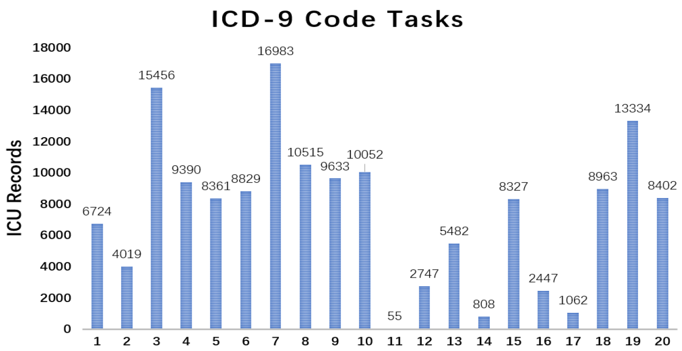As shown in Figure 9, among 190 label pairs in 20 labels, there are 158 label pairs under 0.1, which means the correlation is weak between those labels. Thus, in such a sparse situation, exploiting the feature within a single variable rather than exploiting the relation between labels is more important. VS-GRU can do a better job in keeping the characteristic from a single variable.

4.4.2. Missing Factor in VS-GRU

In order to further discuss the missing factor impact on classification problems, we implement two experiments: replacing the missing factor with missing rate (VS-GRU-$\mu$ and VS-GRU-i-$\mu$) and removing the missing factor from the update functions (VS-GRU w/o $\beta$ and VS-GRU-i w/o $\beta$). To be specific, we replace the missing factor $\beta$ with missing rate $\mu$ in the first layer of VS-GRU-i-$\mu$ and replace the missing factor $\beta$ with $1-\mu$ in penalized mechanism in the second layer. Thus, the variables with a higher missing rate get more punishment. The experimental results are shown in

Table 4. Comparison on the missing factor in a single task.

Model	Mortality Task (PhysioNet)	Mortality Task (MIMIC-III)
VS-GRU	0.8502 ± 0.010	0.8576 ± 0.007
VS-GRU-$\mu$	0.8479 ± 0.006	0.8554 ± 0.007
VS-GRU w/o $\beta$	0.8469 ± 0.014	0.8549 ± 0.008

and

Table 5. Comparison on the missing factor in multi-task.

Model	All 4 Tasks (PhysioNet)	ICD-9 Code Tasks (MIMIC-III)
VS-GRU-i ${}^1$	0.8534 ± 0.018	0.7196 ± 0.003
VS-GRU-i-$\mu$	0.8451 ± 0.008	0.7103 ± 0.002
VS-GRU-i w/o $\beta$	0.8455 ± 0.015	0.7174 ± 0.003

${}^1$ Dynamic imputation mechanism is removed from VS-GRU-i in this task.

. We can see from the results that missing factor is beneficial to model performances. In single-task problems, VS-GRU-$\mu$ outperforms VS-GRU w/o $\beta$. However, the situation is quite the opposite in multi-task problems. We suggest that the reason is that the missing factor is not only used in the update functions in the first layer but also used as penalized mechanism in the second layer of VS-GRU-i. Given the massive missing values in the datasets, the missing rate of many variables is close to 1. The missing factor can learn the slight differences between missing rates and provide more learnable features to the models. In addition, instead of calculating the missing rate using all the records, we calculate the missing rate within the first and last 24 h, which are called VS-GRU-update and VS-GRU-i-update. Then we test the models if we can update the missing rate every 24 h without significant changes in model performance. We execute the two tasks experiments on MIMIC-III using the update models and original models we propose without the dynamic imputation mechanism. We can see from

Table 6. Comparison on the missing rate on MIMIC-III.

Model	Mortality Task	ICD-9 Code Tasks
GRU-D	0.8527 ± 0.003	0.7123 ± 0.003
VS-GRU	0.8588 ± 0.006	—
VS-GRU-update	0.8570 ± 0.007	—
VS-GRU-i	—	0.7196 ± 0.003
VS-GRU-i-update	—	0.7182 ± 0.002

that the performances of VS-GRU and VS-GRU-i stay stable in the case of updating the missing rate.

Figure 10 plots the learned missing factor of 33 variables in PhysioNet. More than half of the variables have an unchanged missing factor during the changing missing rate, which means that the missing rate of these variables may have little impact on this classification task. In other situations, the missing factor decreases as the missing rate increases, which fit the common sense that we should pay more attention to the variables with a low missing rate. This indicates that the characteristics of these variables are related to their observation frequency. However, two variables behave in the opposite way: TropT (missing rate 0.9983) and Urine (missing rate 0.9917). We suggest that variables with relatively high missing rates lack training examples for missing factors to learn the pattern at a low missing rate, resulting in different trends from other variables. In addition, in the test set, the examples of these variables in the low missing rate are rare. It is safe to say that it causes little impact on classification performance.

4.4.3. Deep Supervision in VS-GRU

Deep supervision is designed to improve the training procedure of the time series classification problem, not aiming to address its missing values. To further discuss the modeling ability of multivariate time series with a high missing rate, we separate deep supervision from the model and only use the last time step as supervision. We evaluate it on the four tasks again, comparing it with the strong baseline GRU-D. The best results are highlighted in the following tables.

As

Table 7. Comparison on deep supervision in a single task.

Model	Mortality Task (PhysioNet)	Mortality Task (MIMIC-III)
GRU-D	0.8424 ± 0.012	0.8370 ± 0.012
VS-GRU w/o ds	0.8431 ± 0.012	0.8557 ± 0.007

and

Table 8. Comparison on deep supervision in multi-task.

Model	All 4 Tasks (PhysioNet)	ICD-9 Code Tasks (MIMIC-III)
GRU-D	0.8370 ± 0.012	0.7123 ± 0.003
VS-GRU-i w/o ds ${}^1$	0.8413 ± 0.015	0.7180 ± 0.003

${}^1$ Dynamic imputation mechanism is removed from VS-GRU-i in this task.

show, even without deep supervision, our models still achieve the best results in all four tasks.

5. Conclusions

Few studies on multivariate time series with massive missing values focus on exploiting the univariable missing pattern extraction and utilizing the different missing rate to improve the performance of the classification problem. To address the single-label classification problem, we propose a GRU-based model: VS-GRU. The VS-GRU processes variables separately at first so that a variable with a low missing rate can maintain its feature before being integrated with a variable with a high missing rate. For multi-label classification problems, based on VS-GRU, we propose VS-GRU-i in two GRU layers with penalized mechanisms, which can address multi-task classification problems. In experiments of two real-world public datasets, VS-GRU and VS-GRU-i achieved optimal experimental results in single-label classification tasks and multi-label classification tasks, respectively. We believe that our models are capable of capturing the pattern of time series with massive missing values and are effective in real life in addition to the field of health care.

References

1. Audet, A.M.; Squires, D.; Doty, M.M. Where are we on the diffusion curve? Trends and drivers of primary care physicians’ use of health information technology. Health Serv. Res. 2014, 49, 347–360. [Google Scholar] [CrossRef] [PubMed]
2. Tsay, R.S. Multivariate Time Series Analysis: With R and Financial Applications; John Wiley & Sons: Hoboken, NJ, USA, 2013. [Google Scholar]
3. Häyrinen, K.; Saranto, K.; Nykänen, P. Definition, structure, content, use and impacts of electronic health records: A review of the research literature. Int. J. Med. Inform. 2008, 77, 291–304. [Google Scholar] [CrossRef] [PubMed]
4. Jha, A.K.; DesRoches, C.M.; Campbell, E.G.; Donelan, K.; Rao, S.R.; Ferris, T.G.; Shields, A.; Rosenbaum, S.; Blumenthal, D. Use of electronic health records in US hospitals. N. Engl. J. Med. 2009, 360, 1628–1638. [Google Scholar] [CrossRef] [PubMed]
5. Johnson, A.E.; Pollard, T.J.; Mark, R.G. Reproducibility in critical care: A mortality prediction case study. In Proceedings of the Machine Learning for Healthcare Conference, Boston, MA, USA, 18–19 August 2017; pp. 361–376. [Google Scholar]
6. Choi, E.; Bahadori, M.T.; Schuetz, A.; Stewart, W.F.; Sun, J. Doctor ai: Predicting clinical events via recurrent neural networks. In Proceedings of the Machine Learning for Healthcare Conference, Los Angeles, CA, USA, 19–20 August 2016; pp. 301–318. [Google Scholar]
7. Verburg, I.W.M.; Atashi, A.; Eslami, S.; Holman, R.; Abu-Hanna, A.; de Jonge, E.; Peek, N.; de Keizer, N.F. Which models can I use to predict adult ICU length of stay? A systematic review. Crit. Care Med. 2017, 45, e222–e231. [Google Scholar] [CrossRef] [PubMed]
8. Kang, H. The prevention and handling of the missing data. Korean J. Anesthesiol. 2013, 64, 402. [Google Scholar] [CrossRef] [PubMed]
9. Contreras, J.; Espinola, R.; Nogales, F.J.; Conejo, A.J. ARIMA models to predict next-day electricity prices. IEEE Trans. Power Syst. 2003, 18, 1014–1020. [Google Scholar] [CrossRef]
10. Ralaivola, L.; D’Alché-Buc, F. Time series filtering, smoothing and learning using the kernel Kalman filter. In Proceedings of the 2005 IEEE International Joint Conference on Neural Networks, Montreal, QC, Canada, 31 July–4 August 2005; Volume 3, pp. 1449–1454. [Google Scholar]
11. Che, Z.; Kale, D.; Li, W.; Bahadori, M.T.; Liu, Y. Deep computational phenotyping. In Proceedings of the 21th ACM SIGKDD International Conference on Knowledge Discovery and Data Mining, Sydney, NSW, Australia, 10–13 August 2015; pp. 507–516. [Google Scholar]
12. Lee, J. Patient-specific predictive modeling using random forests: An observational study for the critically ill. JMIR Med. Inform. 2017, 5, e3. [Google Scholar] [CrossRef]
13. Lipton, Z.C.; Kale, D.C.; Elkan, C.; Wetzel, R. Learning to diagnose with LSTM recurrent neural networks. arXiv 2015, arXiv:1511.03677. [Google Scholar]
14. Woolley, S.B.; Cardoni, A.A.; Goethe, J.W. Last-observation-carried-forward imputation method in clinical efficacy trials: Review of 352 antidepressant studies. Pharmacotherapy 2009, 29, 1408–1416. [Google Scholar] [CrossRef]
15. Shi, W.; Zhu, Y.; Philip, S.Y.; Huang, T.; Wang, C.; Mao, Y.; Chen, Y. Temporal dynamic matrix factorization for missing data prediction in large scale coevolving time series. IEEE Access 2016, 4, 6719–6732. [Google Scholar] [CrossRef]
16. Rehfeld, K.; Marwan, N.; Heitzig, J.; Kurths, J. Comparison of correlation analysis techniques for irregularly sampled time series. Nonlinear Processes Geophys. 2011, 18, 389–404. [Google Scholar] [CrossRef] [Green Version]
17. García-Laencina, P.J.; Sancho-Gómez, J.L.; Figueiras-Vidal, A.R. Pattern classification with missing data: A review. Neural Comput. Appl. 2010, 19, 263–282. [Google Scholar] [CrossRef]
18. Lipton, Z.C.; Kale, D.C.; Wetzel, R. Modeling missing data in clinical time series with rnns. arXiv 2016, arXiv:1606.04130. [Google Scholar]
19. Marlin, B.M.; Kale, D.C.; Khemani, R.G.; Wetzel, R.C. Unsupervised pattern discovery in electronic health care data using probabilistic clustering models. In Proceedings of the 2nd ACM SIGHIT International Health Informatics Symposium, Miami, FL, USA, 28–30 January 2012; pp. 389–398. [Google Scholar]
20. Längkvist, M.; Karlsson, L.; Loutfi, A. A review of unsupervised feature learning and deep learning for time-series modeling. Pattern Recognit. Lett. 2014, 42, 11–24. [Google Scholar] [CrossRef] [Green Version]
21. Karim, F.; Majumdar, S.; Darabi, H.; Chen, S. LSTM fully convolutional networks for time series classification. IEEE Access 2017, 6, 1662–1669. [Google Scholar] [CrossRef]
22. Yao, S.; Hu, S.; Zhao, Y.; Zhang, A.; Abdelzaher, T. Deepsense: A unified deep learning framework for time-series mobile sensing data processing. In Proceedings of the 26th International Conference on World Wide Web, International World Wide Web Conferences Steering Committee, Perth, Australia, 3–7 April 2017; pp. 351–360. [Google Scholar]
23. Che, Z.; Purushotham, S.; Cho, K.; Sontag, D.; Liu, Y. Recurrent neural networks for multivariate time series with missing values. Sci. Rep. 2018, 8, 6085. [Google Scholar] [CrossRef]
24. Harutyunyan, H.; Khachatrian, H.; Kale, D.C.; Ver Steeg, G.; Galstyan, A. Multitask learning and benchmarking with clinical time series data. Sci. Data 2019, 6, 96. [Google Scholar] [CrossRef] [PubMed]
25. Akçay, H.; Filik, T. Short-term wind speed forecasting by spectral analysis from long-term observations with missing values. Appl. Energy 2017, 191, 653–662. [Google Scholar] [CrossRef]
26. Soguero-Ruiz, C.; Hindberg, K.; Mora-Jiménez, I.; Rojo-Álvarez, J.L.; Skrøvseth, S.O.; Godtliebsen, F.; Mortensen, K.; Revhaug, A.; Lindsetmo, R.O.; Augestad, K.M.; et al. Predicting colorectal surgical complications using heterogeneous clinical data and kernel methods. J. Biomed. Inform. 2016, 61, 87–96. [Google Scholar] [CrossRef]
27. Soguero-Ruiz, C.; Fei, W.M.; Jenssen, R.; Augestad, K.M.; Álvarez, J.L.R.; Jiménez, I.M.; Lindsetmo, R.O.; Skrøvseth, S.O. Data-driven temporal prediction of surgical site infection. In Proceedings of the AMIA Annual Symposium Proceedings, Chicago, IL, USA, 12–16 November 2015; Volume 2015, p. 1164. [Google Scholar]
28. Futoma, J.; Hariharan, S.; Heller, K. Learning to detect sepsis with a multitask Gaussian process RNN classifier. In Proceedings of the 34th International Conference on Machine Learning-Volume 70, Sydney, NSW, Australia, 6–11 August 2017; pp. 1174–1182. [Google Scholar]
29. Mikalsen, K.Ø.; Bianchi, F.M.; Soguero-Ruiz, C.; Jenssen, R. Time series cluster kernel for learning similarities between multivariate time series with missing data. Pattern Recognit. 2018, 76, 569–581. [Google Scholar] [CrossRef] [Green Version]
30. Mikalsen, K.Ø.; Soguero-Ruiz, C.; Bianchi, F.M.; Revhaug, A.; Jenssen, R. Time series cluster kernels to exploit informative missingness and incomplete label information. arXiv 2019, arXiv:1907.05251. [Google Scholar]
31. Yoon, J.; Zame, W.R.; van der Schaar, M. Estimating missing data in temporal data streams using multi-directional recurrent neural networks. IEEE Trans. Biomed. Eng. 2018, 66, 1477–1490. [Google Scholar] [CrossRef] [PubMed]
32. Le Gall, J.R.; Lemeshow, S.; Saulnier, F. A New Simplified Acute Physiology Score (SAPS II) Based on a European/North American Multicenter Study. JAMA 1993, 270, 2957–2963. [Google Scholar] [CrossRef] [PubMed]
33. Vincent, J.L.; Moreno, R.; Takala, J.; Willatts, S.; De Mendonça, A.; Bruining, H.; Reinhart, C.K.; Suter, P.M.; Thijs, L.G. The SOFA (Sepsis-related Organ Failure Assessment) score to describe organ dysfunction/failure. Intensive Care Med. 1996, 22, 707–710. [Google Scholar] [CrossRef] [PubMed]
34. Knaus, W.A.; Zimmerman, J.E.; Wagner, D.P.; Draper, E.A.; Lawrence, D.E. APACHE-acute physiology and chronic health evaluation: A physiologically based classification system. Crit. Care Med. 1981, 9, 591–597. [Google Scholar] [CrossRef] [PubMed]
35. Dybowski, R.; Gant, V.; Weller, P.; Chang, R. Prediction of outcome in critically ill patients using artificial neural network synthesised by genetic algorithm. Lancet 1996, 347, 1146–1150. [Google Scholar] [CrossRef]
36. Kim, S.; Kim, W.; Park, R.W. A comparison of intensive care unit mortality prediction models through the use of data mining techniques. Healthc. Inform. Res. 2011, 17, 232–243. [Google Scholar] [CrossRef] [PubMed]
37. Strauman, A.S.; Bianchi, F.M.; Mikalsen, K.Ø.; Kampffmeyer, M.; Soguero-Ruiz, C.; Jenssen, R. Classification of postoperative surgical site infections from blood measurements with missing data using recurrent neural networks. In Proceedings of the 2018 IEEE EMBS International Conference on Biomedical & Health Informatics (BHI), Las Vegas, NV, USA, 4–7 March 2018; pp. 307–310. [Google Scholar]
38. Purushotham, S.; Meng, C.; Che, Z.; Liu, Y. Benchmarking deep learning models on large healthcare datasets. J. Biomed. Inform. 2018, 83, 112–134. [Google Scholar] [CrossRef]
39. Che, Z.; Purushotham, S.; Li, G.; Jiang, B.; Liu, Y. Hierarchical deep generative models for multi-rate multivariate time series. In Proceedings of the International Conference on Machine Learning, Vienna, Austria, 13–18 July 2018; pp. 783–792. [Google Scholar]
40. Bahadori, M.T.; Lipton, Z.C. Temporal-Clustering Invariance in Irregular Healthcare Time Series. arXiv 2019, arXiv:1904.12206. [Google Scholar]
41. Shukla, S.N.; Marlin, B. Interpolation-Prediction Networks for Irregularly Sampled Time Series. In Proceedings of the ICLR, Vancouver, BC, Canada, 30 April–3 May 2018. [Google Scholar]
42. Silva, I.; Moody, G.; Scott, D.J.; Celi, L.A.; Mark, R.G. Predicting in-hospital mortality of icu patients: The physionet/computing in cardiology challenge 2012. In Proceedings of the 2012 Computing in Cardiology, Krakow, Poland, 9–12 September 2012; pp. 245–248. [Google Scholar]
43. Johnson, A.E.; Pollard, T.J.; Shen, L.; Lehman, L.-W.H.; Feng, M.; Ghassemi, M.; Moody, B.; Szolovits, P.; Celi, L.A.; Mark, R.G. MIMIC-III, a freely accessible critical care database. Sci. Data 2016, 3, 160035. [Google Scholar] [CrossRef] [Green Version]
Figure 1. Example of clinical time series with six variables within 12 time steps. Red dots denote the observation marks.
Applsci 09 03041 g001
Figure 2. GRU structure (symbol in red refers to input).
Applsci 09 03041 g002
Figure 3. VS-GRU (symbol in red refers to input and symbol in blue refers to decay mechanism).
Applsci 09 03041 g003
Figure 4. VS-GRU-i with deep supervision.
Applsci 09 03041 g004
Figure 5. Missing rate of 33 variables in PhysioNet. x-axis, missing rate, y-axis, variable id in PhysioNet. maximum missing rate: 0.9985, minimum missing rate: 0.1161, average missing rate: 0.8193.
Applsci 09 03041 g005
Figure 6. The label distribution in all four tasks. x-axis, label id in all four tasks, 1: in-hospital mortality, 2: length-of-stay less than 3 days, 3: whether the patient had a cardiac condition, 4: whether the patient was recovering from surgery; y-axis, the number of ICU records with positive labels.
Applsci 09 03041 g006
Figure 7. Missing rate of 99 variables in MIMIC-III. x-axis, missing rate, y-axis, variable id in MIMIC-III. maximum missing rate: 0.9997, minimum missing rate: 0.7406, average missing rate: 0.9559.
Applsci 09 03041 g007
Figure 8. The label distribution in ICD-9 Code tasks. x-axis, label id in the ICD-9 diagnosis category; y-axis, the number of ICU records with positive labels.
Applsci 09 03041 g008
Figure 9. The Pearson correlation coefficient between labels in ICD-9 Code tasks on MIMIC-III. x-axis, the label pair id in ICD-9 Code tasks; y-axis, Pearson correlation coefficient between labels.
Applsci 09 03041 g009
Figure 10. Learned missing factor of 33 variables in PhysioNet.
Applsci 09 03041 g010