Article

A XGBoost Model with Weather Similarity Analysis and Feature Engineering for Short-Term Wind Power Forecasting

College of Science, Northwest A&F University, Yangling 712100, China
*
Author to whom correspondence should be addressed.
Appl. Sci. 2019, 9(15), 3019; https://doi.org/10.3390/app9153019
Submission received: 22 June 2019 / Revised: 17 July 2019 / Accepted: 25 July 2019 / Published: 26 July 2019
(This article belongs to the Section Energy Science and Technology)

Abstract

:
Large-scale wind power access may cause a series of safety and stability problems. Wind power forecasting (WPF) is beneficial to dispatch in advance. In this paper, a new extreme gradient boosting (XGBoost) model with weather similarity analysis and feature engineering is proposed for short-term wind power forecasting. Based on the similarity among historical days’ weather, k-means clustering algorithm is used to divide the samples into several categories. Additionally, we also create some time features and drop unimportant features through feature engineering. For each category, we make predictions using XGBoost. The results of the proposed model are compared with the back propagation neural network (BPNN) and classification and regression tree (CART), random forests (RF), support vector regression (SVR), and a single XGBoost model. It is shown that the proposed model produces the highest forecasting accuracy among all these models.

1. Introduction

Renewable energy has been a popular choice for power generation and has become a crucial part in government development schemes. Wind energy is a kind of clean and pollution-free renewable energy source and its reserves are huge. By 2008, wind power production was about 94.1 million kilowatts globally, which is more than 1% of the world’s power generation. There is no doubt that wind power generation plays an important role in electric power systems [1,2]. However, wind power generation faces primary problems of intermittency and uncertainty. The randomness of wind is caused by a variety of factors, such as terrain, season, air pressure, temperature, and so on, which can cause many problems [3]. Fluctuations in wind speed and large-scale wind power grid-connected access threaten the safe and stable operation of the power system and have a bad effect on electricity dispatching, which increases the operating costs of the power system and means the economic benefits of wind power generation decrease. The experience of wind power operation in various countries shows that wind power forecasting (WPF) technology is one of the most effective ways to alleviate the pressure of power grids by adjusting peak-loads and reducing system reserve capacity.
At present, wind power forecasting (WPF) systems can be divided into three categories, which include short-term forecasting, medium-term forecasting, and long-term forecasting [4]. Short-term forecasting predicts the wind power from several hours to one week, medium-term forecasting predicts the wind power from one week to one month, while long-term forecasting forecasts the wind power from several months to one year.
WPF methods consist of physical approaches, statistic approaches, learning approaches, and combination forecasting approaches [5]. Physical approaches mainly consider physical quantities, such as numerical weather, wind turbine hub height, wind turbine thrust coefficient, and other technical parameters [6]. The aim is to find the optimal wind speed estimation at the hub height of the wind turbine and convert it into the output power of the wind farm according to the power curve of the wind turbine or wind farm. Statistical methods can be divided into two categories. One category establishes linear or nonlinear mapping of wind power system input and output by curve fitting and parameter estimation based on previous wind power, including the autoregressive moving average (ARMA) model [7], autoregressive integrated moving average (ARIMA) model [8], and generalized autoregressive conditional heterosked (GARCH) model [9]. The other category builds the regression model between meteorological observations and wind power. Examples include support vector regression (SVR) [10,11,12,13], classification and regression tree (CART) [14], Gaussian process regression (GPR) [15], and ensemble learning [16]. The learning approaches are mainly based on the artificial neural network (ANN) [17], which uses meteorological observations provided by the wind farm to predict the wind power; examples include back propagation neural network (BPNN) [18,19], radial basis function neural network (RBFNN) [20], deep belief network (DBN) [21], recurrent neural network (RNN) [22], long short-term memory (LSTM) [23], and other neural networks [24,25,26]. For ANN, the adjustment of parameters may have a great influence on the prediction results. Some optimization algorithms are also used in combination with neural networks to adjust the parameters of neural networks to achieve better prediction results [27]. Combination forecasting approaches are based on a variety of different prediction models to overcome the shortcomings of a single model and obtain higher accuracy by using the combination of different models’ prediction results [28].
In this paper, we present a new WPF model based on XGBoost, weather similarity analysis, and feature engineering. We try to analyze the similarity of weather and assign meteorological observation data into several clusters. Next, when we consider the influence of weather features, we also think about time features. We create some time features and select some more important features in feature engineering. The features we select are the inputs of XGBoost. For each type, we train a XGBoost model. Then, we compute the forecasting accuracy for short-term forecasting, showing that the proposed model has a better performance than BPNN, CART, random forests (RF), support vector regression (SVR), and a single XGBoost model.
The remaining parts of this paper are organized as follows. An overview of the XGBoost algorithm is outlined in Section 2. Section 3 introduces the details of the proposed WPF model. Simulation results obtained by the proposed model and other compared methods are shown in Section 4. The final section gives the conclusions.

2. Methodology

XGBoost is applied to supervised learning problems using training data to predict the target variables [29]. XGBoost selects decision tree as its base learner. By adding new base learners, the error between predictive values and target are reduced. The final predictive values are equal to the summation of all base learners.
XGBoost algorithm can be regarded as an additive model consisting of M decision trees, which are given by Equation (1):
Y i = m = 1 M f m ( x i ) ,     f m F
where f stands for a decision tree and F represents the function of all decision trees.
In the process of regression, the object function of the additive model becomes (2):
Obj ( θ ) = i = 1 n l ( y i ,   Y i ) + m = 1 M Ω ( f m ) ,     θ = ( f 1 , f 2 , , f M )
where l means loss function and Ω expresses the regularization term.
For regularization terms of every decision tree, we improve the decision tree using vector mapping. Therefore, the details of Ω(f) can be seen in Equation (3):
Ω ( f ) =   γ T + 1 2 λ j = 1 T ω j 2
where T indicates the number of a decision tree’s leaf nodes, ω represents the vector of score, and both γ and λ express the penalty factor.
XGBoost uses the forward stagewise algorithm to simplify the model complexity. Each time the model adds a decision tree, it learns one new function and its coefficients to fit the last step predicted residuals. Therefore, when the tth step learning happens, the predictive value of xi: Y i t = Y i t 1 + f t ( x i )   . Therefore, the object function should be expressed by Equation (4):
Obj ( θ ) t = i = 1 n l ( y i ,   Y i t ) + m = 1 t Ω ( f m )   = i = 1 n l ( y i ,   Y i t 1 + f t ( x i ) ) + m = 1 t Ω ( f m )  
Based on object function, the XGBoost algorithm applies the greedy algorithm to build the decision tree; by building decision trees constantly, a complete XGBoost model is established.

3. Model Establishment

In this section, the detailed process of the proposed model is discussed, which consists of data preprocessing, weather similarity analysis, and feature engineering.

3.1. Data Preprocessing

Due to errors in data collection, there may be some unreasonable values in the original data. These unreasonable data will decrease the prediction accuracy, which is not conducive to establishing the model to predict wind power. Besides, data preprocessing can provide a good preliminary understanding of the data, so the first step of the model is to preprocess the data.
  • Data cleaning: There are outliers in the original data. For example, there are some points in the original data, whose corresponding wind speed is equal to zero, but the corresponding wind power is smaller than zero. It is obvious that these data are unreasonable and need to be cleaned.
  • Missing data filling: After data cleaning is completed, there will be gaps in the data. It is necessary to fill these missing values, because if the filling of missing values is reasonable, the prediction accuracy of the model can be improved. The k-Nearest Neighbor (KNN) algorithm is adopted to find the nearest neighbor in the time series to fill the missing values in the data.
  • Data normalization: The purpose of data normalization is to reduce the influence of order of magnitude on the model, accelerate the training speed of the model, and make the model more accurate than before. Min-max normalization maps data between zero and one, whose transformation formula is described by Equation (5):
    x = x x m i n x m a x x m i n
Data cleaning, filling of missing data, and data normalization constitute data preprocessing. The three steps above are significant for improving the prediction accuracy of the model.

3.2. Weather Similarity Analysis

From the perspective of weather similarity, we analyze the relationship among meteorological observations at different times and classify weather into several categories based on meteorological observations data from the wind farm, which contains wind speed, wind direction, temperature, air pressure, and humidity. For each type of weather, a wind power prediction model is established.
For the preprocessed meteorological observations data, the k-means algorithm is used to accomplish the classification of weather. The k-means algorithm finds k clusters from the dataset and the number of k clusters is decided by users. Every cluster is described by its centroid, which is the center of all points belonging to this cluster. The inputs of the k-means algorithm include wind speed, wind direction, temperature, pressure, and humidity. First, k points are selected randomly as centroids of k clusters. Then, each point of the dataset is assigned to a cluster. Then, the nearest centroid for each point of the dataset is found and assigned to the cluster corresponding to the nearest centroid. Next, let the centroids of different clusters be equal to the center of all points belonging to this cluster. Repeat the above operations until the centroids of different clusters are unchanged. The number of clusters is determined by cross-validation. The value of k corresponds to the best WPF results.
The pseudo code of the above process is in Algorithm 1 [30].
Algorithm 1. K-means Algorithm
Input: Dataset S = {x1, x2, …, xh}
Procedure:
1: select k samples from dataset S as the original centroid vector c = { c1, c2, …, ck }
2: for every sample xi then
3: calculate the euclidean distance between xi and cj (j = 1,2,…,k)
4: find the nearest centroid cj and let ui = j where ui represent the corresponding cluster of xi
5: end for
6: u = { u1, u2, …, uk }
7: for every cluster then
8: calculate the centroid of every cluster vi
9: end for
10: v = { v1, v2, …, vk }, u = {u1, u2, …, uh}
11: if v == c then
12: return u
13: else
14: c = v and go to step 2
15: end if
Output: vector u which shows the cluster label of every sample

3.3. Feature Engineering

The data determines the upper limit of machine learning, and the algorithm approximates this upper limit as much as possible. Feature engineering refers to the process of transforming raw data into training data for the model. Its purpose is to obtain better training data characteristics. The first thing we need to do is extract more features from the original data. We suppose that wind power is associated with some time features. Then, we create some time features, such as day of the week and hour of day. In addition to these above features, we guess that the current wind power may be related to the wind power from 24 and 48 h earlier. All supposed time features are created. The details of these time features could be found in Table 1.
We then create certain features, and in Figure 1, the Pearson correlation coefficient matrix is expressed as a heatmap. The Pearson correlation coefficient can describe the linear correlation between two features. We find that some features we created have a stronger linear correlation with other features, for example, “month” and “doy”. According to the message of the heatmap, the Pearson correlation coefficient between these two features approaches one. Two features with complete linear correlation can be expressed by each other, which means that the contained information of these two features have no differences. For the two features with strong linear correlation, removing one of them can improve the accuracy of the model with less data information loss. Therefore, we drop the “month” feature.
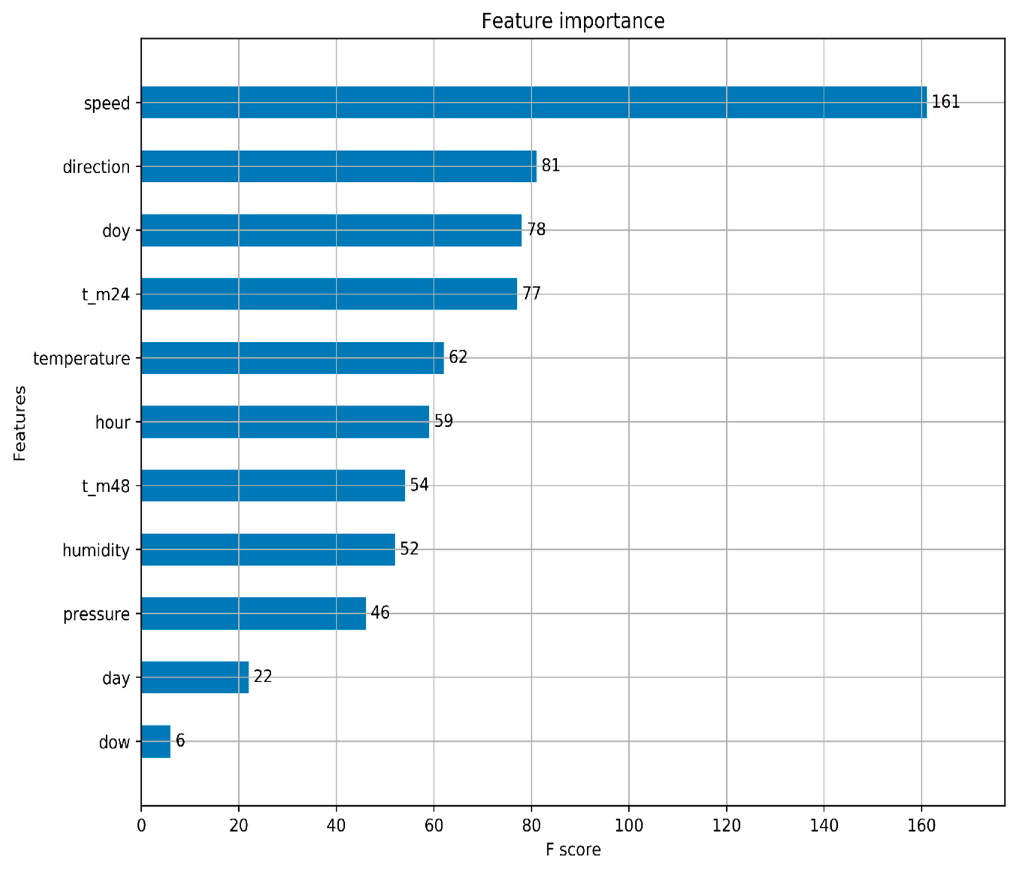
However, the process of filtering features is not still over. Here, we continue to select features with help from XGBoost. First, we use all features to build a model based on XGBoost. Then, we calculate the value of importance of every feature. The value of importance indicates how much this feature affects the model based on XGBoost. In Figure 2, the F score represents the value of importance. Based on the value of importance, we drop some features whose value of importance is smaller than other features. In Figure 2, the two features are “day” and “dow”, whose F scores are significantly smaller than other features. Therefore, for the model based on XGBoost, these two features play an unimportant role in forecasting. In other words, these two features have a weaker correlation with wind power than other features. Consequently, these two features containing “day” and “dow” are dropped. In the end, the input features of XGBoost are composed of “speed”, “direction”, “doy”, “t_m24”, “temperature”, “hour”, “t_m48”, “humidity”, and “pressure”.

3.4. The Structure of Proposed Model

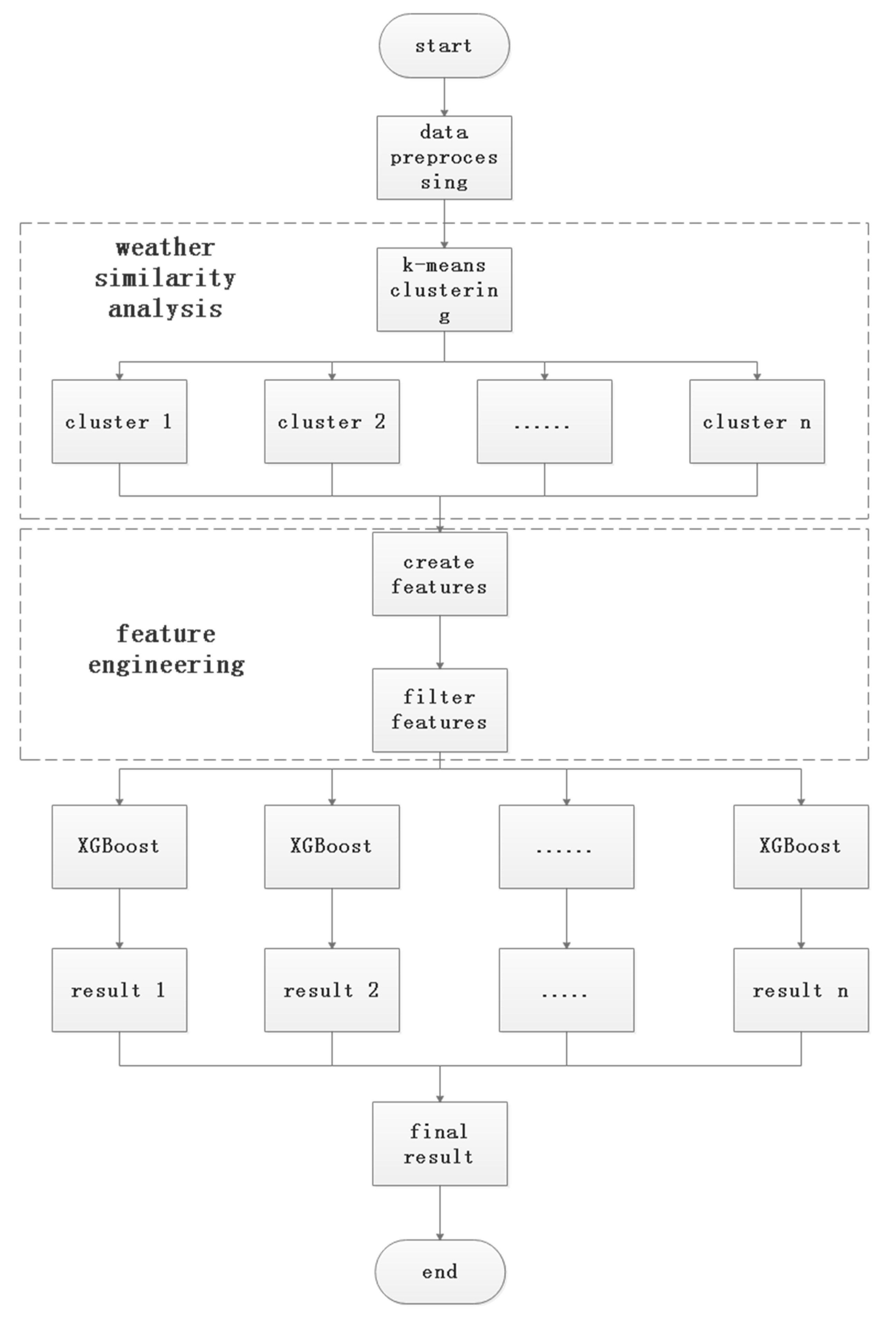
In this paper, we divide the preprocessed data into several clusters. For every cluster, we build a model based on XGBoost. Through feature engineering, we obtain the features that will be regarded as the inputs of the XGBoost algorithm. After the training process of XGBoost, our model is established successfully. Since the XGBoost algorithm has some parameters, it is necessary to adjust the parameters for more higher accuracy. Ten-fold cross-validation is used to test algorithm accuracy and adjust parameters here. First, we divide the original data into ten parts. We choose one part as the testing data and others as training data at a time. We obtain the results of ten different choices. The mean value of the results is the final evaluation indicator. A set of parameters corresponding to the best result are the parameters we use. The proposed model is simulated by using Python and the structure of this model is shown in Figure 3.

4. Experiments

4.1. Description of Data

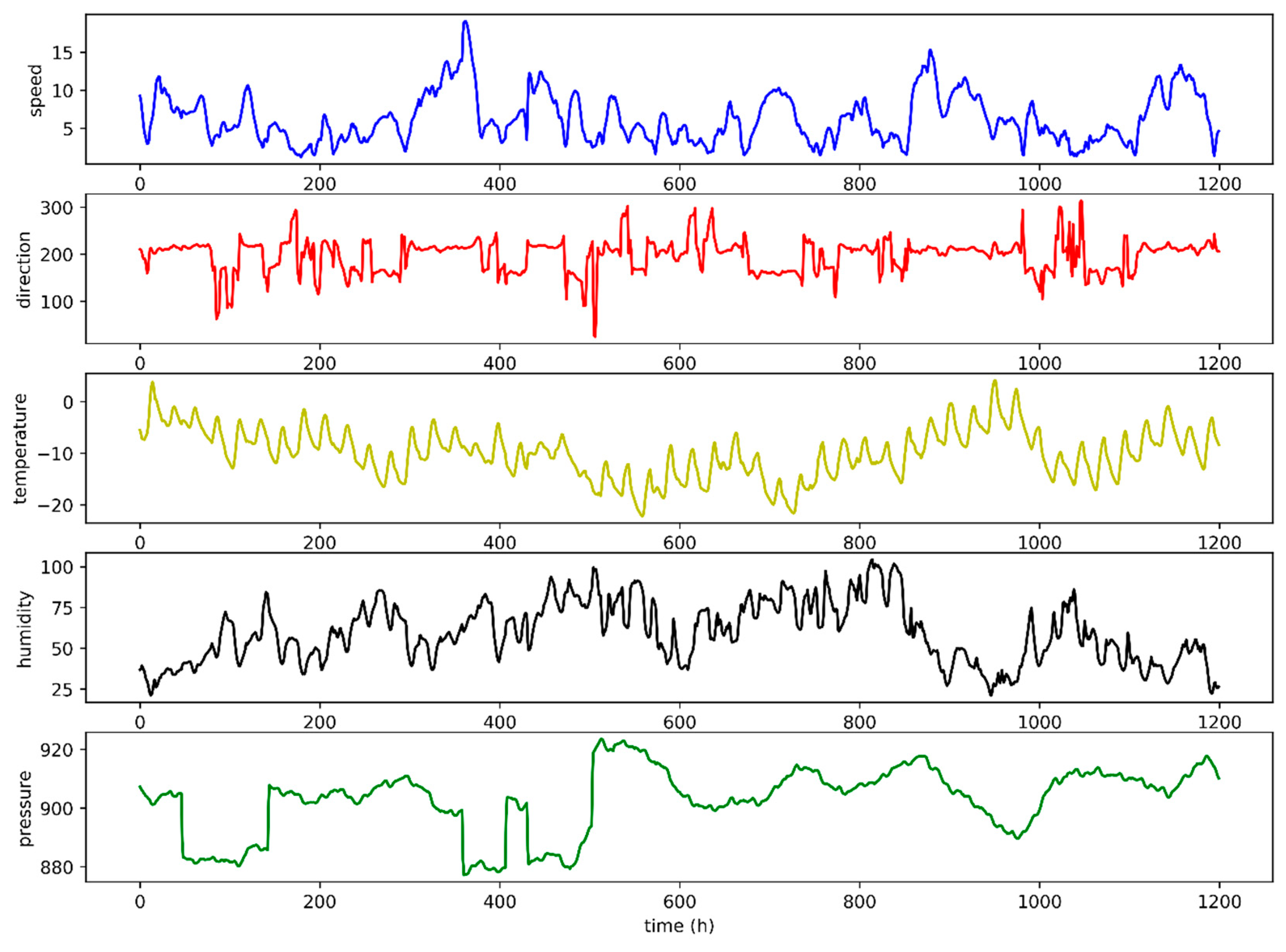
In this paper, the data is provided by a wind farm in northwest China’s Gansu province. The raw data contains timestamp, wind power, wind speed, wind direction, air pressure, temperature, and humidity data each hour from January 1, 2016, to April 28, 2017. Figure 4 shows the change of different meteorological observations of normalized data over time in the first 50 days. The five curves in Figure 4 represent the normalized values of wind speed, wind direction, temperature, humidity, and air pressure, respectively. As shown in Figure 4, some meteorological observations have obvious volatility, especially wind speed, temperature, and humidity. These features are characterized by periodic variations, which explain that the correlation between meteorological observations and time is strong and it is necessary to create some time features. According to the introduction section, we need to predict the wind power from several hours to one week based on previous data for short-term wind power forecasting. In this paper, we predict wind power per hour for the next week, which has 168 values. Therefore, the testing set uses the data from April 21, 2017, to April 28, 2017, and the training set uses the data from January 1, 2016, to April 20, 2017, in specific experiments.

4.2. Evaluating Indicator

For short-term wind power forecasting, mean square error (MSE), root mean square error (RMSE), mean absolute error (MAE), and root mean absolute error (RMAE) are the most common evaluation indicators, which can be illustrated by:
M S E = 1 n i = 1 n ( P P i P M i ) 2
R M S E = 1 n i = 1 n ( P P i P M i ) 2
M A E = 1 n i = 1 n | P P i P M i |
R M A E = 1 n i = 1 n | P P i P M i |
where n is the number of samples, PMi is real time power, and PPi is forecasting wind power. mean square error (MSE) is the average sum of the difference between the real value and the predicted value. root mean square error (RMSE) is used to measure the deviation between the observed value and the truth value. For MSE and RMSE, mean absolute error (MAE), and root mean absolute error (RMAE) are not susceptible to outliers and can better reflect the actual situation of predicted error. These four indicators will be used in testing part.

4.3. Wind Power Forecasting Results

In order to better express the value of the proposed model in this paper, five models are selected to be compared with the proposed model. These models include CART, BPNN, RF, SVR, and a simple XGBoost model.
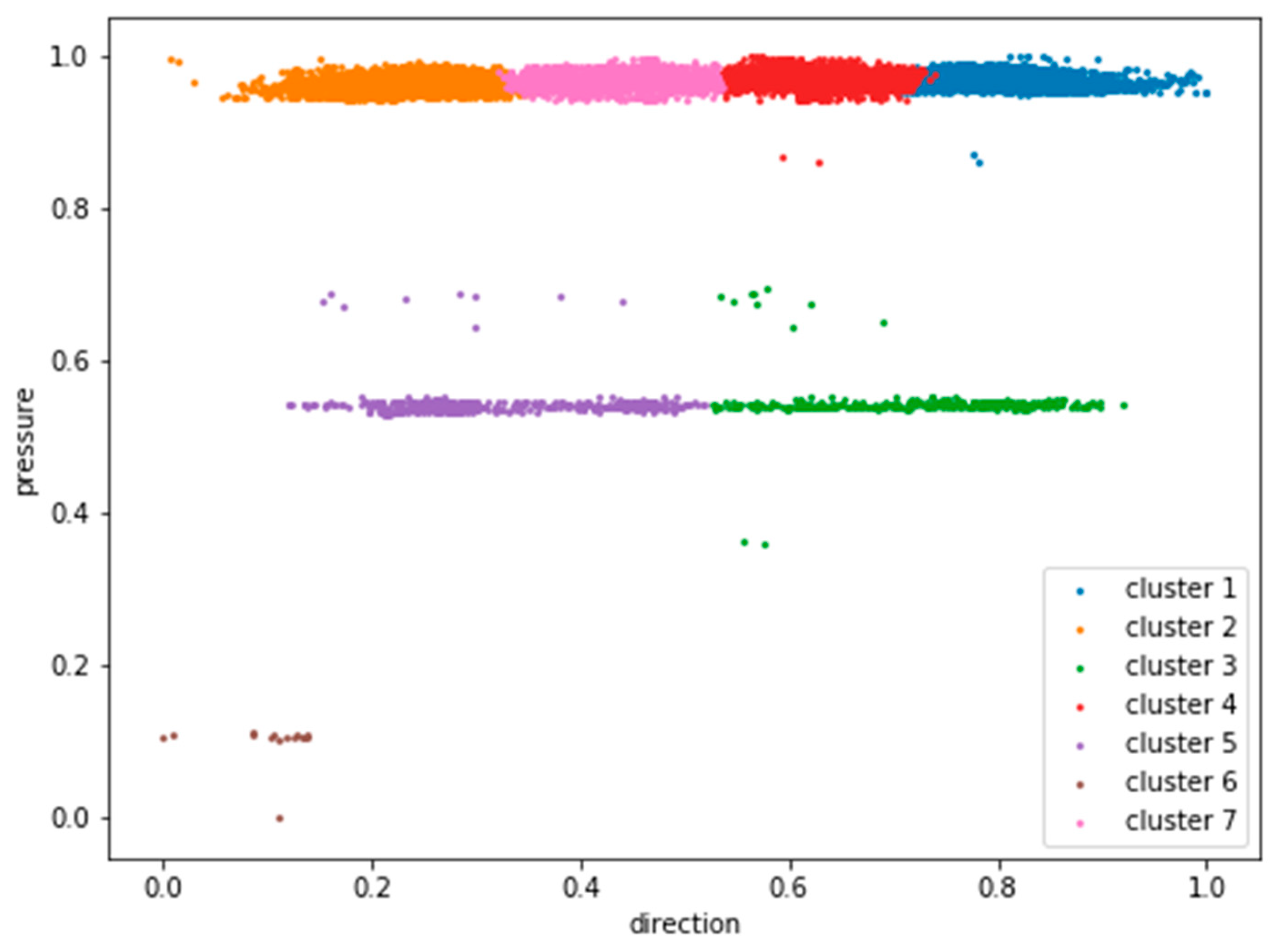
Figure 5 shows the clustering results. Points with different colors represent different clusters. We can clearly see that there are seven clusters in Figure 5. These clusters have different characteristics, such as different wind directions and different air pressure. From the prediction results in Table 2, we see that the XGBoost model with weather similarity analysis and feature engineering can reduce the prediction error compared with a single XGBoost model, in which MSE, RMSE, MAE, and RMAE are reduced by 19.93%, 10.52%, 18.79%, and 9.73%, respectively. From this point of view, weather similarity analysis and feature engineering improve the accuracy of forecasting results significantly. What is more, the proposed model is the most accurate model among the six models. For RF, which obtains the best performance among the five compared models, MSE, RMSE, MAE, and RMAE are reduced by 16.56%, 8.68%, 4.58%, and 2.11%, respectively.
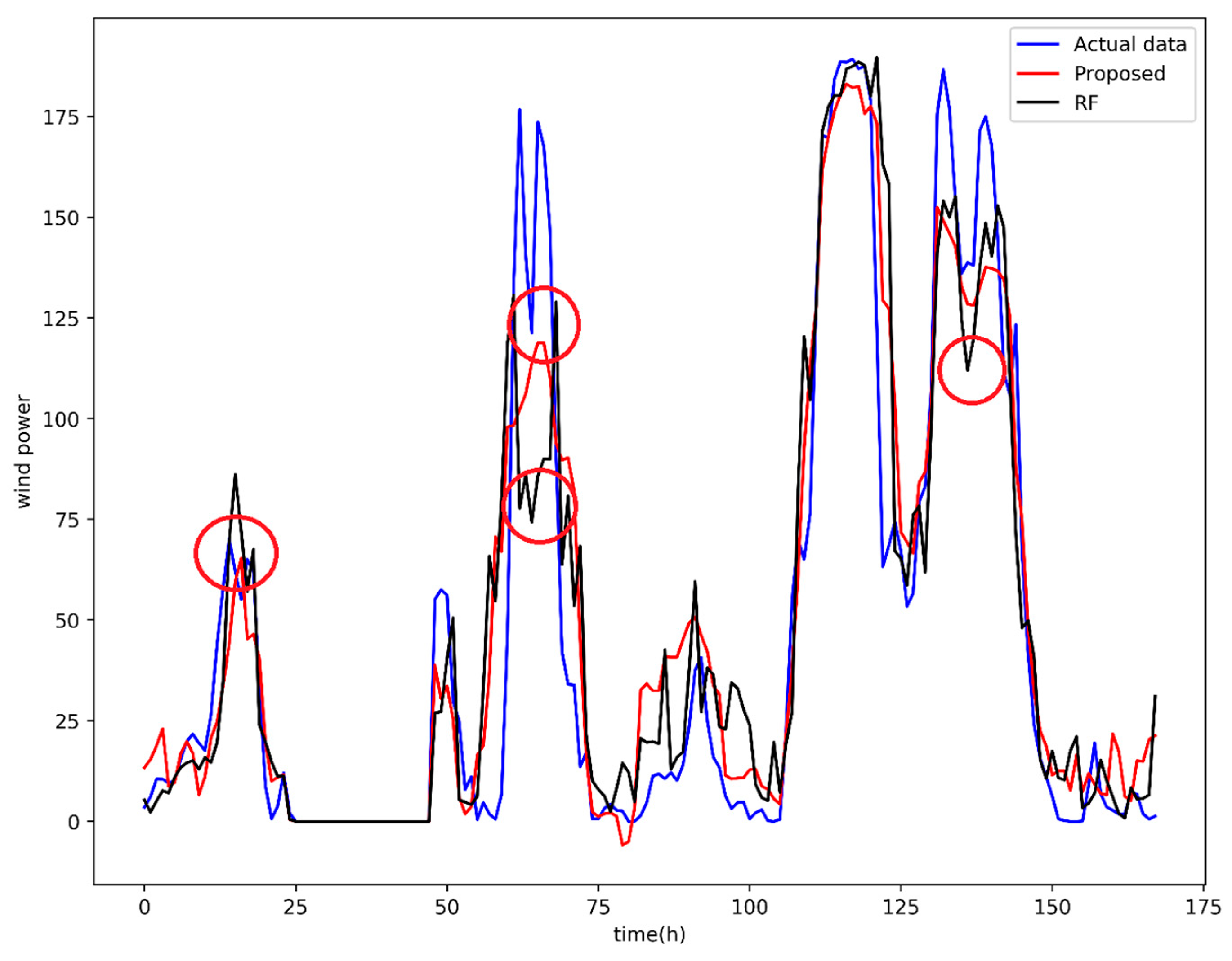
Figure 6 shows the predicted wind power of RF and the proposed model from April 21, 2017, to April 28, 2017. For the five compared models, there is a RF model in Figure 6, because RF is the best model among all compared models based on results in Table 2. In Figure 6, the blue curve represents wind power of actual data. The red curve represents wind power forecasting results of the proposed model and the black curve represents wind power forecasting results of RF. According to the messages of the red circle in Figure 6, it is easy to see that the proposed model is obviously better than RF.
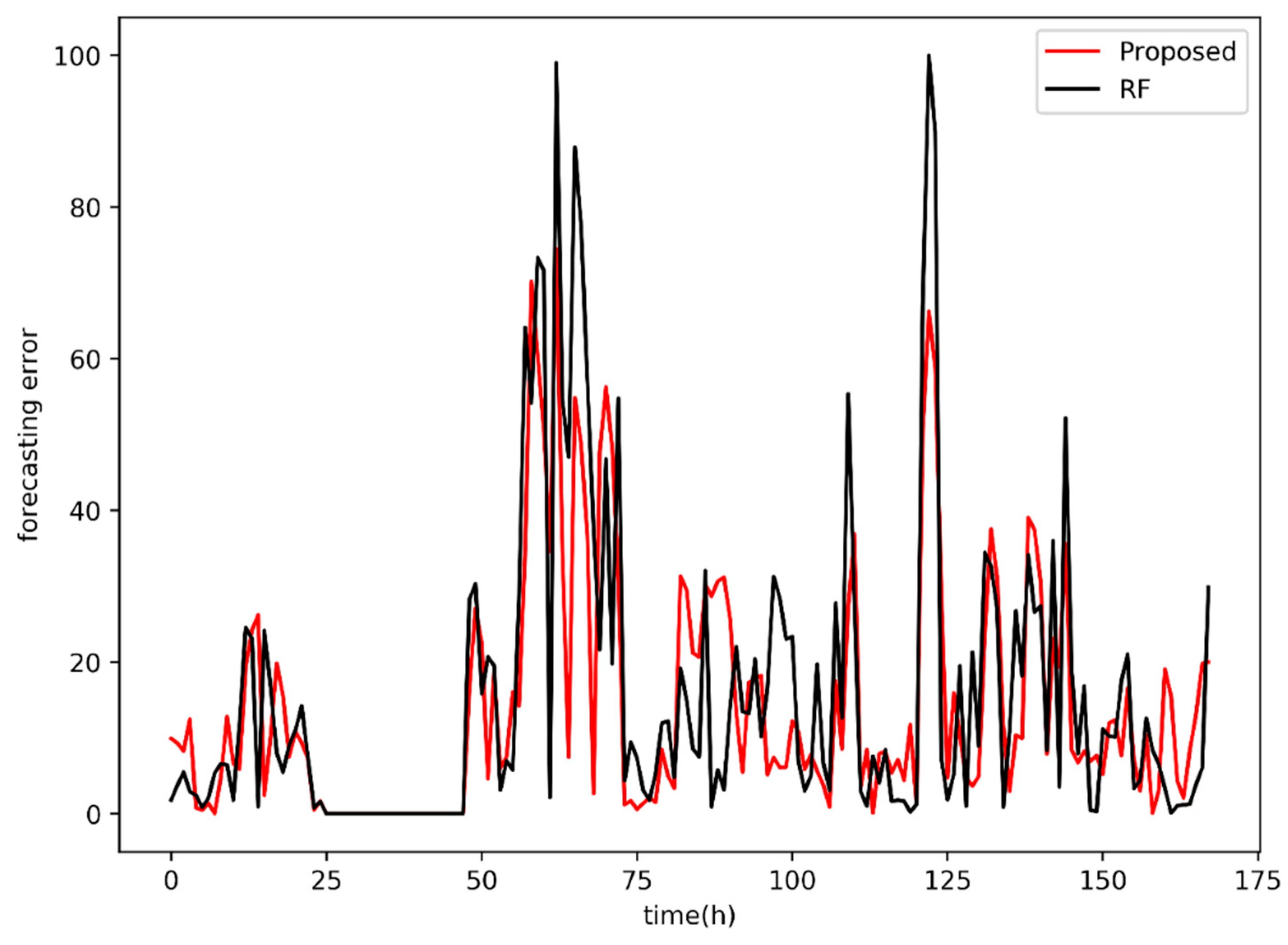
Figure 7 displays the absolute error between actual wind power and predictive wind power for different models. In Figure 7, the red curve represents the absolute error between the predictive wind power of the proposed model and actual wind power, and the black curve represents the absolute error between the predictive wind power of RF and actual wind power. For most times, the forecasting error of the RF is greater than the proposed model. The proposed model can follow the wind power’s variation tendency of actual data and the stability of the proposed model is better than RF.
According to the above analysis, it is significant to see that the XGBoost model with weather similarity analysis and feature engineering is better than a simple XGBoost model. This also confirms the value of weather similarity analysis and feature engineering. In short, the proposed model in this paper is better than the traditional WPF models (BPNN, CART, RF, XGBoost, and SVR) and has wide applicability.

5. Conclusions

WPF plays a crucial part in solving intermittency and uncertainty of wind. An accurate WPF model is important for electrical power systems to complete the advance dispatching of electricity. In this paper, a new model for short-term wind power forecasting has been proposed, which consists of XGBoost, weather similarity analysis, and feature engineering. In the proposed model, we analyze weather similarity based on the k-means clustering algorithm and classify meteorological observation data into several clusters. In order to improve the accuracy of forecasting, we create some time features and select some features that are more important than others. Then, XGBoost, whose inputs contain all of the features we obtained from feature engineering, is used for prediction. Next, the WPF results are compared to RF, CART, BPNN, SVR, and a simple XGBoost model to fully evaluate the performance of the proposed model. According to the simulation results, it is obvious that the proposed model does have the highest accuracy of prediction for short-term forecasting. However, there are still some problems that need to be considered for the proposed model. For example, some spatial features can also be added in the WPF model, such as environmental and geographic features near the wind farm. The question still remains of how to achieve feature selection with more potential features. These points are valuable and important in further studies.

Author Contributions

H.Z. performed the experiment and wrote the paper. Y.W. helped in the experiments and writing.

Funding

This research was funded by programs for the fundamental research funds of the central university, grant number Z109021561, and Northwest A&F University students’ innovative entrepreneurial training plan program, grant number 201910712040.

Conflicts of Interest

The authors declare no conflict of interest.

References

  1. Okumus, I.; Dinler, A. Current status of wind energy forecasting and a hybrid method for hourly predictions. Energy Convers. Manag. 2016, 123, 362–371. [Google Scholar] [CrossRef]
  2. Zhao, Y.; Ye, L.; Li, Z.; Song, X.; Lang, Y.; Su, J. A novel bidirectional mechanism based on time series model for wind power forecasting. Appl. Energy 2016, 177, 793–803. [Google Scholar] [CrossRef]
  3. Xia, S.; Chan, K.W.; Luo, X.; Bu, S.; Ding, Z.; Zhou, B. Optimal sizing of energy storage system and its cost-benefit analysis for power grid planning with intermittent wind generation. Renew. Energy 2018, 122, 472–486. [Google Scholar] [CrossRef]
  4. Zhang, Y.; Wang, J.; Wang, X. Review on probabilistic forecasting of wind power generation. Renew. Sustain. Energy Rev. 2014, 32, 255–270. [Google Scholar] [CrossRef]
  5. Costa, A.; Crespo, A.; Navarro, J.; Lizcano, G.; Madsen, H.; Feitosa, E. A review on the young history of the wind power short-term prediction. Renew. Sustain. Energy Rev. 2008, 12, 1725–1744. [Google Scholar] [CrossRef]
  6. Ma, L.; Luan, S.; Jiang, C.; Liu, H.; Zhang, Y. A review on the forecasting of wind speed and generated power. Renew Sustain. Energy Rev. 2009, 13, 915–920. [Google Scholar]
  7. Lu, J.; Wang, B.; Ren, H.; Zhao, D.; Wang, F.; Shafie-khah, M.; Catalao, J.P.S. Two-Tier Reactive Power and Voltage Control Strategy Based on ARMA Renewable Power Forecasting Models. Energies 2017, 10, 1518. [Google Scholar] [CrossRef]
  8. Shi, J.; Qu, X.; Zeng, S. Short-Term Wind Power Generation Forecasting: Direct Versus Indirect Arima-Based Approaches. Int. J. Green Energy 2011, 8, 100–112. [Google Scholar] [CrossRef]
  9. Chen, H.; Li, F.; Wang, Y. Wind power forecasting based on outlier smooth transition autoregressive GARCH model. J. Mod. Power Syst. Clean 2018, 6, 532–539. [Google Scholar] [CrossRef]
  10. Salcedo-Sanz, S.; Ortiz-Garcia, E.G.; Perez-Bellido, A.M.; Portilla-Figueras, A.; Prieto, L. Short term wind speed prediction based on evolutionary support vector regression algorithms. Expert. Syst. Appl. 2011, 38, 4052–4057. [Google Scholar] [CrossRef]
  11. Ortiz-Garcia, E.G.; Salcedo-Sanz, S.; Perez-Bellido, A.M.; Gascon-Moreno, J.; Portilla-Figueras, J.A.; Prieto, L. Short-term wind speed prediction in wind farms based on banks of support vector machines. Wind Energy 2011, 14, 193–207. [Google Scholar] [CrossRef]
  12. Yang, L.; He, M.; Zhang, J.; Vittal, V. Support-Vector-Machine-Enhanced Markov Model for Short-Term Wind Power Forecast. IEEE Trans. Sustain. Energy 2015, 6, 791–799. [Google Scholar] [CrossRef]
  13. Ranganayaki, V.; Deepa, S.N. SVM Based Neuro Fuzzy Model for Short Term Wind Power Forecasting. Natl. Acad. Sci. Lett. 2017, 40, 131–134. [Google Scholar] [CrossRef]
  14. Gonzalez, C.; Mira-McWilliams, J.; Juarez, I. Important variable assessment and electricity price forecasting based on regression tree models: Classification and regression trees, Bagging and Random Forests. IET Gener. Transm. Dis. 2015, 9, 1120–1128. [Google Scholar] [CrossRef]
  15. Fang, S.; Chiang, H. A High-Accuracy Wind Power Forecasting Model. IEEE Trans. Power Syst. 2017, 32, 1589–1590. [Google Scholar] [CrossRef]
  16. Lahouar, A.; Slama, J.B.H. Hour-ahead wind power forecast based on random forests. Renew. Energy 2017, 109, 529–541. [Google Scholar] [CrossRef]
  17. Li, T.; Li, Y.; Liao, M.; Wang, W.; Zeng, C. A New Wind Power Forecasting Approach Based on Conjugated Gradient Neural Network. Math. Probl. Eng. 2016, 2016. [Google Scholar] [CrossRef]
  18. Huang, D.; Gong, R.; Gong, S. Prediction of Wind Power by Chaos and BP Artificial Neural Networks Approach Based on Genetic Algorithm. J. Electr. Eng. Technol. 2015, 10, 41–46. [Google Scholar] [CrossRef] [Green Version]
  19. Wang, J.; Fang, K.; Pang, W.; Sun, J. Wind Power Interval Prediction Based on Improved PSO and BP Neural Network. J. Electr. Eng. Technol. 2017, 12, 989–995. [Google Scholar] [CrossRef] [Green Version]
  20. Chang, W. An RBF Neural Network Combined with OLS Algorithm and Genetic Algorithm for Short-Term Wind Power Forecasting. J. Appl. Math. 2013, 2013. [Google Scholar] [CrossRef]
  21. Wang, K.; Qi, X.; Liu, H.; Song, J. Deep belief network based k-means cluster approach for short-term wind power forecasting. Energy 2018, 165, 840–852. [Google Scholar] [CrossRef]
  22. Shi, Z.; Liang, H.; Dinavahi, V. Direct Interval Forecast of Uncertain Wind Power Based on Recurrent Neural Networks. IEEE Trans. Sustain. Energy 2018, 9, 1177–1187. [Google Scholar] [CrossRef]
  23. Liu, Y.; Guan, L.; Hou, C.; Han, H.; Liu, Z.; Sun, Y.; Zheng, M. Wind Power Short-Term Prediction Based on LSTM and Discrete Wavelet Transform. Appl. Sci. 2019, 9, 1108. [Google Scholar] [CrossRef]
  24. Salcedo-Sanz, S.; Perez-Bellido, A.M.; Ortiz-Garcia, E.G.; Portilla-Figueras, A.; Prieto, L.; Paredes, D. Hybridizing the fifth generation mesoscale model with artificial neural networks for short-term wind speed prediction. Renew. Energy 2009, 34, 1451–1457. [Google Scholar] [CrossRef]
  25. Hervas-Martinez, C.; Salcedo-Sanz, S.; Gutierrez, P.A.; Ortiz-Garcia, E.G.; Prieto, L. Evolutionary product unit neural networks for short-term wind speed forecasting in wind farms. Neural. Comput. Appl. 2012, 21, 993–1005. [Google Scholar] [CrossRef]
  26. Salcedo-Sanz, S.; Perez-Bellido, A.M.; Ortiz-Garcia, E.G.; Portilla-Figueras, A.; Prieto, L.; Correoso, F. Accurate short-term wind speed prediction by exploiting diversity in input data using banks of artificial neural networks. Neurocomputing 2009, 72, 1336–1341. [Google Scholar] [CrossRef]
  27. Jiang, P.; Li, X.; Dong, Y. Research and Application of a New Hybrid Forecasting Model Based on Genetic Algorithm Optimization: A Case Study of Shandong Wind Farm in China. Math. Probl. Eng. 2015, 2015, 14. [Google Scholar] [CrossRef]
  28. Nielsen, H.A.; Nielsen, T.S.; Madsen, H.; San Isidro Pindado, M.J.; Marti, I. Optimal combination of wind power forecasts. Wind Energy 2007, 10, 471–482. [Google Scholar] [CrossRef]
  29. Pang, L.; Wang, J.; Zhao, L.; Wang, C.; Zhan, H. A Novel Protein Subcellular Localization Method With CNN-XGBoost Model for Alzheimer’s Disease. Front. Genet. 2018, 9, 751. [Google Scholar] [CrossRef]
  30. Jain, A.K. Data clustering: 50 years beyond K-means. Pattern Recognit. Lett. 2010, 31, 651–666. [Google Scholar] [CrossRef]
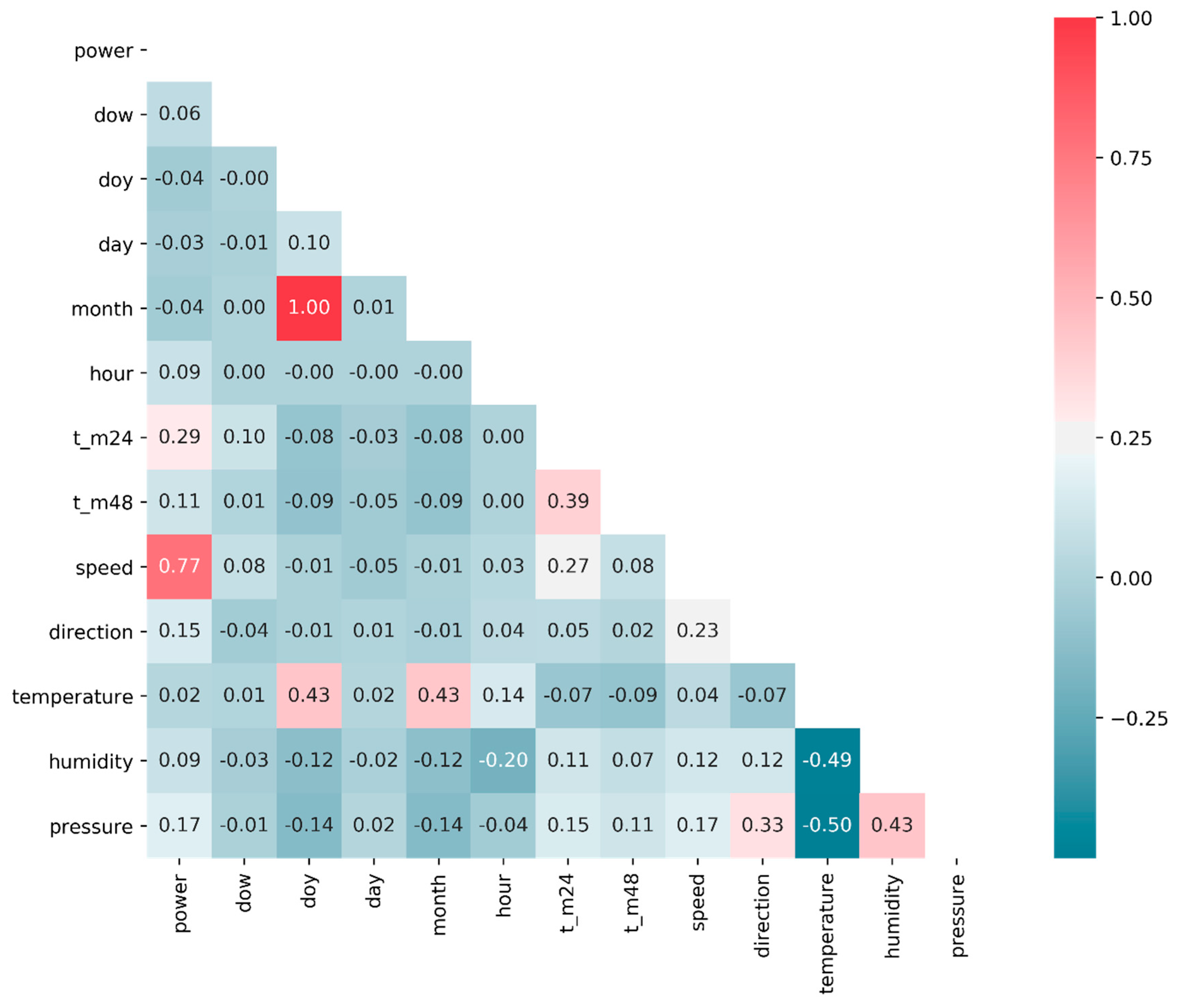
Figure 1. Heatmap of Pearson correlation coefficient matrix.
Applsci 09 03019 g001
Figure 2. The value of importance for each feature.
Applsci 09 03019 g002
Figure 3. The structure of our model.
Applsci 09 03019 g003
Figure 4. Line chart of different weather features.
Applsci 09 03019 g004
Figure 5. Scatter diagram of clustering results.
Applsci 09 03019 g005
Figure 6. WPF results of RF and the proposed model.
Applsci 09 03019 g006
Figure 7. Absolute error between actual wind power and predictive results of different models.
Applsci 09 03019 g007
Table 1. Meaning of different time features.
FeatureMeaning
dowday of the week (integer 0–6)
doyday of the year (integer 0–365)
dayday of the month (integer 1–31)
monthmonth of the year (integer 1–12)
hourhour of the day (integer 0–23)
minuteminute of the day (integer 0–1339)
t_m24wind power value from 24 h earlier
t_m48wind power value from 48 h earlier
Table 2. Evaluated results of different wind power forecasting models.
ProposedRFCARTBPNNXGBoostSVR
MSE434.06520.20948.51738.97542.111174.73
RMSE20.8322.8131.5127.1823.2834.27
MAE13.7414.4019.3920.3716.9223.37
RMAE3.713.794.404.514.114.83
RF: random forests; CART: classification and regression tree; BPNN: back propagation neural network; XGBoost: extreme gradient boosting; SVR: support vector regression; MSE: mean square error; RMSE: root mean square error; MAE: mean absolute error; RMAE: root mean absolute error.