Article

Power Grid Reliability Evaluation Considering Wind Farm Cyber Security and Ramping Events

1
College of Electrical Engineering, Sichuan University, Chengdu 610065, China
2
Department of Electrical Engineering, Southern Methodist University, Dallas, TX 75275, USA
3
College of Electrical and Information Engineering, Hunan University, Changsha 410000, China
*
Author to whom correspondence should be addressed.
Appl. Sci. 2019, 9(15), 3003; https://doi.org/10.3390/app9153003
Submission received: 15 June 2019 / Revised: 11 July 2019 / Accepted: 24 July 2019 / Published: 26 July 2019

Abstract

:
The cybersecurity of wind farms is an increasing concern in recent years, and its impacts on the power system reliability have not been fully studied. In this paper, the pressing issues of wind farms, including cybersecurity and wind power ramping events (WPRs) are incorporated into a new reliability evaluation approach. Cyber–physical failures like the instantaneous failure and longtime fatigue of wind turbines are considered in the reliability evaluation. The tripping attack is modeled in a bilevel optimal power flow model which aims to maximize the load shedding on the system’s vulnerable moment. The time-varying failure rate of wind turbine is approximated by Weibull distribution which incorporates the service time and remaining life of wind turbine. Various system defense capacities and penetration rates of wind power are simulated on the typical reliability test system. The comparative and sensitive analyses show that power system reliability is challenged by the cybersecurity of wind farms, especially when the installed capacity of wind power continues to rise. The timely patching of network vulnerabilities and the life management of wind turbines are important measures to ensure the cyber–physical security of wind farms.

1. Introduction

As the predominant source of renewable energy until 2017, global wind power capacity has expanded 11% to 539 GW [1]. The dynamic performance and reliability of power systems are increasingly relying on the operation of wind farms. However, the cybersecurity of wind farms is challenged by their simple and reliable communication protocols, fixed control flows, long-update cycles of software, and stable topologies [2]. On the one hand, the operation of a wind farm is affected by the intermittence of wind speed and the low inertia of wind turbines (WTs). On the other hand, the cyber threats of a wind farm bring new uncertainties that lead to the abnormal operation and undesired-tripping of WTs. For the secure and reliable operation of a power grid, it is very necessary to develop reliable evaluation methods that incorporate the cyber security of wind farms.
To quantify the availability and relationship of the cyber–physical effects [3] of a wind farm, a multi-state Markov model [4,5] was broadly applied. Furthermore, graphical methods were developed for a better expression of the cyber–physical relationship, such as the stochastic Petri net [6], the Bayesian network [7], the complex network [8], and the attack tree [9]. Though the cyber–physical relationship has been modeled by different approaches, it is challenging to quantify the frequency of attacks and system defense mechanisms. Yichi Zhang et al. [10] proposed a preliminary study of cyber-attack effects on power grid reliability. The forced outage modes of critical components caused by a cyber-attack were investigated. Data driven approaches have also been popular to estimate the time to compromise or restore the vulnerabilities of an information network [11]. The mean time-to-compromise (MTTC) the vulnerabilities is a widely used unit to quantify the frequency of cyber-attacks [7,12,13]. Once the probabilities of a cyber-attack and its cyber–physical relationship are determined, the states of cybersecurity can be sampled for further reliability analysis.
Thus far, there has been a lot of investigation and research on the cybersecurity of wind farms. However, most of them have not considered the impact of cyber-attacks on power grid reliability. In [14], the attack scenarios involving WTs control, wind farm disruption and substation disruption were discussed in detail. The dynamic simulation of a WT was tested in [15], and the impact caused by malicious modifications on the WT control parameters was discussed. In [16], power system reliability, considering the sudden tripping of WTs, was evaluated via a reliability analysis. With the specific attack paths, the MTTC was applied to estimate the frequency of cyber-attacks. However, the contributions of system defense is rarely considered. Though the tripping attack results in great harm to power systems, it is fortunately and usually one-off and unsustainable. Nowadays, a growing concern is the intention to damage the WTs rather than stop them. If the control system of WTs is intruded, the malicious command can mislead the WTs to run in a dangerous state. The impacts of cyber-attacks against the mechanical components of WTs should be further investigated.
Wind power ramping events (WPRs) [17] are typically known as a cause of large power fluctuations. The load shedding resulted from WPRs exceeded 1000 MW/year according to the report of the Electricity Reliability Council of Texas system [18]. Uncertainties associated with wind power integration challenge the operational adequacy of conventional power systems. The modeling of WPRs, especially the feature of ramping rate [19], should be fully considered to evaluate the operational adequacy of power systems. To address those problems, the main contributions of this paper are as follows: (i) A stochastic attack–defense model is proposed to estimate the frequency of cyber-attacks. (ii) Two typical attack scenarios, including an imperfect attack, are modeled to assess the impact of cybersecurity in the wind farm. (iii) A wind power model that considers the ramping rate is proposed and incorporated into a composite power reliability evaluation. The remainder of this paper is organized as follows. Section 2 introduces the typical communication architecture and risk of cybersecurity in the wind farms. In Section 3, the stochastic models for a state sampling of cyber-attacks and system defenses are proposed. The scenarios, including a worst-case attack and an imperfect attack (IPA), on WTs are illustrated in Section 4. In Section 5, the flow of reliability evaluation is constructed, and case studies are presented in Section 6. Finally, conclusions as well as research discussion are summarized.

2. Wind Farm Cyber Architecture and Security Risks

The diagram in Figure 1 is a typical communication network of a wind farm. The WTs use cables to transmit data to a local network of the wind power plant. Within a specified zone, several wind farm management systems are connected to a main control center. As the backup of the main control center, the remote control center is connected to the wide area network of wind farm supervisory control and data acquisition (SCADA) systems. As International Electrotechnical Commission (IEC) 61400-25 and IEC 61850-7 specify the uniformed Internet Protocol based communication standards, the equipment and system operation of wind farm are supported by SCADA protocols such as the Object Linking and Embedding for Process Control, Modbus/Transmission Control Protocol or vendor-specific protocols. And the conventional network is supported by the protocols of Telnet, File Transfer Protocol, and HyperText Transfer Protocol.
Wind farm cyber security risks mainly come from the cyber–physical access to the core equipment of wind farm SCADA and energy management system (EMS). As shown in Figure 1, in order to gain the privilege to control a WT, the potential attack paths can be achieved by intruding: (1) The wind turbine control panel (WTCP); (2) the operating and control local area network (LAN) of wind farms; (3) the control center LAN of wind farms; and (4) the remote control LAN in the substation [16].
The WTCP is a vulnerable node in the control network of a wind farm. Once the pin of a WTCP is cracked, the operating and control data of a WT can be monitored and revised. Additionally, the fiber optics or switches of a WTCP can be physically accessed by microcomputers. Generally, wind turbines are linked in a ring topology communication network [14]. The failure of one link has no impact on the others. However, in linear or star topology, by compromising the terminal or central WT, it is possible to intercept legitimate command and control messages to mislead the operation of dozens, possibly hundreds, of wind turbines.
A virtual private network (VPN) is provided to vendors for devices or software services and is another vulnerable point of the cybersecurity. The remote access of a VPN with outdated and unencrypted protocols can be used by attacker to reach the wind farm control LAN. Real-time command and measurement information can be revised on the workstation. Similarly, through a VPN, both the wind farm control center and remote control are at risk of being intruded. If the Inter-Control Center Communications Protocol (ICCP) server and SCADA server are compromised, the attacker could gain the privilege to obstruct the operation of wind farms. The attacker could change the output of the WT, inject false data [20], or instigate an emergency shutdown, which could be a hard stop that induces excessive wear and tear on critical mechanical components. In this paper, the occurrence of cyber-attacks was modeled as the competition result between compromising and fixing the cyber vulnerabilities. The consequent operating and physical states of WTs were projected on the system reliability evaluation.

3. Attack–Defense Model of Vulnerability

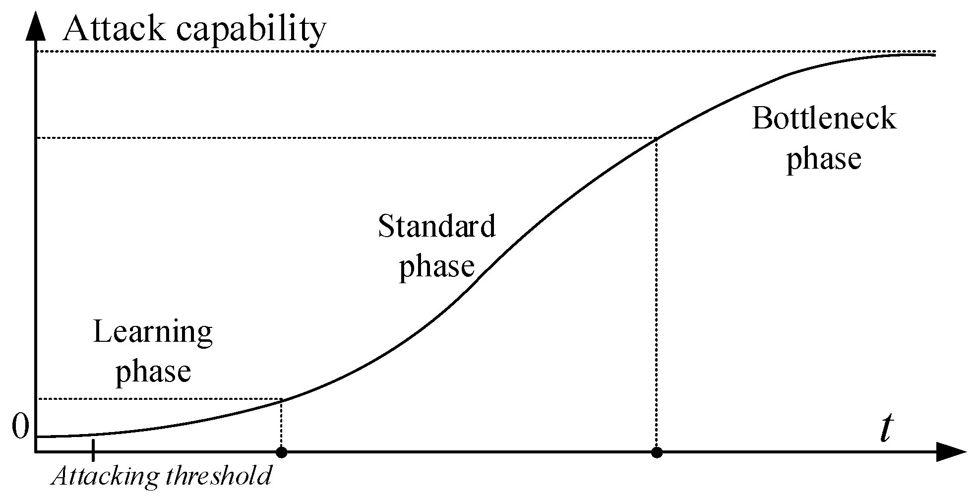
3.1. Stochastic Model Based on MTTC

The mean time-to-compromise (MTTC) [12] under a specific condition is defined to represent the average time required for cyber-attacks. The attack could be an exploiting of the vulnerabilities of a target. For a single known/unknown vulnerability, its potential impacts and complexity could be preliminary evaluated by the Common Vulnerability Scoring System (CVSS) [21]. The scores of vulnerabilities have been used as empirical data [12] to evaluate the time for compromising vulnerabilities. When the attack paths of a specific network are determined, the mean time to compromise all the vulnerabilities leading to the goal could be quantified as the time to attack the entire network [16]. The MTTC can be defined as:
M T T C ( c ) = x i X T ( x i ) p ( x i c ) p ( c )
where T(xi) is the time for exploiting the vulnerability xi, p(xi Λ c) is the probability that the vulnerability xi which leads to the attack target is compromised, and p(c) represents the probability that the attack target is reached.
Though the MTTC model provides a reference for estimating the time of attacks, it is limited by the specific attack graph which is challenging to apply to generic conditions. Additionally, the MTTC does not consider the process of system defense. During the attack, if some of the vulnerabilities are patched by defense software, the cyber-attack will be delayed or prevented. Thus, both the attack and defense process should be considered in estimating the occurrence of attacks. Based on the existing MTTC, a flexible cumulative distribution function (CDF) of attack time is developed for the reliability evaluation. In this paper, the attack and defense process were modeled separately.
Based on the behavior of attacker, [22] divided the attack process into three different phases. According to the typical attacking process introduced in [22], the relationship between the time and attack capability is shown as Figure 2. For a malicious intrusion, a low-skilled attacker would start by raising the skill level. In the learning phase, the attackers have no threats for the target system. After a period of time, the attackers are ready for documented vulnerabilities and available codes in the standard phase. Their destructive capacity increases exponentially. When all standard attack methods are tested, the attacking process enters a bottleneck phase. In this phase, the attackers must find new solutions and try to exploit unknown vulnerabilities. The whole relationship between time and attack capacity approximately conforms to the Laplace distribution [23]. To represent the time characteristics of a cyber-attack in different stages, the equation for estimating the attack probability spending ta is proposed as Equation (2). The probability follows a Laplace distribution ta~L(µ,b).
F a ( t a ) = 1 2 + 1 2 sgn ( t a μ ) ( 1 exp ( | t a μ | b ) )
where Fa(ta) is the probability for attacker spending ta to compromise the vulnerability, µ is the MTTC provided by the history records, and b is the scale parameter of Laplace distribution. A smaller b means a higher probability that t > MTTC.

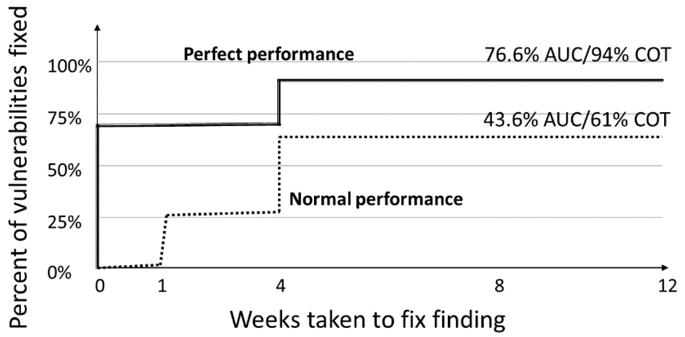
3.2. System Defense Model

The contribution of a system defense can be also measured in terms of time. Generally, the defense mechanism of a power system keeps patching the vulnerabilities of the system network. According to Verizon’s 2017 Data Breach Investigations Report [24], most organizations complete their vulnerabilities patching in 12 weeks. Each patching process could be presented as two indices: The area under the curve (AUC) and the percentage completed on time (COT), as shown in Figure 3. The AUC reveals the overall input of defense progress in 12 weeks, while the COT is the amount of vulnerabilities patched at the cut-off time. Figure 3 illustrates how the vulnerability scan findings of two typical organizations are fixed. The top line represents the performance of an organization with an excellent cyber-defense mechanism. The bottom line is the normal performance of most organizations. As the figure shows, the time feature of vulnerability fixing is similar to a step process. It qualitatively changes after a fixed period, such as the first week and the fourth week. Once the system defense agency patches the vulnerability, the related attack is prevented immediately. In this manner, the defense process of a power system is extracted as a multi-segmented step function, given by (3). According to the investigation of fixing vulnerabilities in [24], four typical system defense parameters are extracted in Table 1. Thus, the security state of system Sa could be described by the difference of attack and defense time as Equation (4), namely the difference of F a 1 and F d 1 , which are the results of inverse functions in Equations (2) and (3), respectively. By sampling the times of Sa = −1, the probability of cyber-attack can be estimated. For example, if the MTTC is 80 days and the scale parameter of Laplace distribution is 50, the probabilities of a cyber-attack can be estimated as listed in Table 2.
F d ( t d ) = { α 0 t d t 1   α 1 t 1 < t d t 2     α 2 t 2 < t d t 3   β t d > t 3
S a = sgn ( F a 1 ( x ) F d 1 ( x ) ) , 0 x 1
where Fd is the probability for the system to fix the vulnerability with time td. The t1, t2, and t3 are the duration for different stages of the system defense. Generally, the defense capability of a cyber-system changes by a week, a month, and the third month. α0, α1, α2 and β are the probabilities to fix the vulnerability on different stages. x is the probability of time for attack or defense. When Sa is positive, it means the time of attack is longer than the defense, so the system defense is successful.

4. Attack Scenarios

To quantify the consequences of cyber-attacks, two attack strategies scenarios were analyzed. The first scenario was the worst-case attack which trips the WT to maximize the load shedding on the system’s vulnerable moment. The second scenario was the imperfect attack, which aims to accelerate the aging and fatigue of a WT. These two attack scenarios affect power system reliability in different time scales. The worst-case attack directly leads to a serious power imbalance, which is a short-term impact to the power system. The IPA increases the failure rate of a WT and deteriorates system reliability in a long term.

4.1. Worst-Case Attack of Wind Turbines

Considering the most severe possible outcome that occurs in a power system, the worst-case attack in this paper was designated as the one which trips a WT on a vulnerable moment of a power system and leads to the worst power imbalance. In order to locate the vulnerable moment, an index of active power margins has been proposed in [16]. The power system takes a higher risk for load shedding when the active power margin stays at lower level during the attack. However, the index does not consider the output of wind power. As the attack target, the running state of the WT should be monitored on the evaluation of the vulnerable moment. Only when the output of the WT is high is the impact of tripping attack is obvious. In this paper, the index was further extended as:
V a ( t ) = P g e n ( t ) + P w ( t ) P l o a d ( t )
where Va(t) is the active power margin of power system at time t. Pgen and Pw are the conventional generation capacity and the total output of wind farms, respectively. Pload is the total load power.
The power system suffers the greatest loss with a minimum value of Va(t) when the tripping attack is launched. The estimation of the tripping moment based on Equation (5) requires the attacker to accurately handle information such as the total conventional generation capability, the wind power output, and the load demand. Though the rationality of the worst-case setting is controversial, the accuracy of load forecasting needs a strict data foundation, and the schedule of power dispatch is challenging to obtain. From the perspective of system reliability, the worst case exposes the greatest impact of cyber-attacks in a conservative way. In this paper, the active power margin prediction was assumed to be obtained by the attackers.

4.2. Long-Term Imperfect Attack of Wind Turbine

Since wind power equipment is designed for lightness and efficiency but is often fragile, the attacker probably launches an IPA to damage the physical states of wind turbines. An IPA is characterized by strong concealment, long duration, and uncertain damage. The impact of an IPA is similar to the Stuxnet attack in the uranium hexafluoride centrifuges in Iran’s Natanz facility [25]. Investigation [26] and review [27] presented the failure statistics of a wind turbine, indicating that most wind turbine failures are caused by the failure of gearboxes and their bearings. Running in critical speed or overloading the operation of a wind turbine can accelerate the fatigue of the mechanical part and even destroy the WT. Excessive load and overheating are the most frequent reason for the premature fatigue of a WT bearing. For example, when the temperature is in excess of 400 °F, the ring and ball materials are annealed [28]. The hardness of the bearing and the state of the lubricant then deteriorate.
Since bearing wear is the most common cause of a WT fault, the impact of an IPA can be quantified by the estimation of the WT bearing state. In this paper, the wear process of a bearing infected was modeled as a continuous degenerative process that obeys the Gamma distribution [29]. The Markov chain [5] was utilized to estimate the states of bearing in different stages. Combining the physical state and service time of bearing, the failure rates of a WT can be further estimated for system reliability evaluation.
Table 3 presents the wearing conditions of a WT bearing, where Δmax = R0Rmin. R0 is the size of new bearing. Rmin is the minimum size allowed for the bearing to operate. Suppose the set of the bearing states is Si at time ti. The time domain state of bearing is x(t) after a short time Δt. The change value of time domain state is yt), and the according state of bearing changes to Sj. The transition probability from Si to Sj is formulated as Equation (6). The probabilities of bearing states can be obtained by iterations of the Markov process as shown in Equation (7).
P i j ( t ) = P { ζ j 1 x ( t ) + y ( Δ t i ) ζ j 1 | ζ i 1 x ( t i ) ζ i } = ζ i 1 ζ i ζ i 1 X ( t ) ζ i X ( t ) f [ y ( Δ t i ) ] f [ x ( t ) ] d y d x ζ i 1 ζ i f [ x ( t ) ] d x
S n = S 0 P ( n ) = S 0 P n
where f(x) is the probability density function of the state increment. ζi and ζj are the state top and bottom limitation, where i = 1, 2, … n; j = i, i + 1, … i + n. S0 is the initial state of bearing. P is the transition matrix, and n is the number of state transitions.
To evaluate the consequence of an IPA, the acceleration fatigue of a bearing is measured by its equivalent operation time (hours). The impact of an IPA is transformed to a time calculation problem. When the sum of normal working hours and the extra equivalent time caused by an attack exceed the boundary of state transition, the transfer times “n” should increase in the Markov process, as shown in Equation (8). Then, the WT’s remaining life can be estimated as the duration between the current state and the failure state.
n = n a Δ t I P A + t s Δ t t r
where n is the number of bearing state transitions, na is the sampled number of the IPA, and ΔtIPA is the equivalent running time caused by attack. In this paper, the ΔtIPA was set as 1.5 times the actual running time of a WT in a day, namely 36 h. ts is the service time of bearing, and Δttr is the time of state transition. Under normal operating conditions, the time of state transition is approximately equal to one tenth of the bearing rated life.
From the viewpoint of system, an IPA increases the failure rate of a WT. The model of time-varying failure rate incorporating the service time and life of a WT can be built as Equation (9), which is the fault probability density function based on the Weibull distribution [30]. When the rated life of a WT is shortened by ΔTa, the failure rate is increased accordingly. In the random failure period, the probability of WT failure state PG can be described by Markov process as Equation (10). With the combined analysis of bearing wear and failure rate, the time-varying failure state of a WT could be obtained. By sampling and updating the states of a WT in the optimal power flow (OPF) model, the impact of an IPA could be quantified in the system reliability assessment.
λ a ( t ) = β ( η Δ T a ) β t β 1
P G ( t ) = λ a λ a + μ λ a λ a + μ e ( λ a + μ ) t
where β is the Weibull exponent and η is the rated lives of WTs. λa and µ are the real time fault rate and repair rate, respectively.

5. Power System Reliability Assessment

In this section, the model of wind power and wind power ramping is proposed. The output and states of WTs are further contained in a bi-level OPF model, which is used to quantify the consequence of a worse-case attack. Then, the flows of a system reliability assessment, considering both a worst-case attack and an IPA, are established.

5.1. Modeling of Wind Power and WPRs

The modeling of wind power is composed by the average output of WTs and power variation results from WPRs. The output of WTs is formulated as Equation (11).
P W ( t ) = { P W 0 0 t T s P W 0 + R W ( t Δ t ) Δ t T s < t T s + D
where PW(t) is the active power of a single WT, PW0 is the annual mean output of wind power, RW is the ramping rate of wind power, Ts is the start time of WPRs, and D is its duration.
R ¯ W ( t ) = 1 Λ C w γ Λ R γ ( t ) C γ
Generally, wind speed varies with different topography. We assumed that the same wind farm would have only one wind speed. If more than one ramping event happens at the same time, the ramping rate can be equivalent to an arithmetic mean, as shown in Equation (12). R ¯ w is the equivalent ramping rate of wind power, Rγ(t) is the ramping rate of wind farm γ at time t, Cγ is the installed capacity of wind farm γ, and Λ and Cw are the number and the total power capacity of wind farms, respectively.
During a ramping event, those generators with ramping rates lower than WPRs cannot contribute to the power regulation. During a ramping event, the available power capacities of generators are less or equal to the maximum power capacity, as shown in Equation (13).
P ¯ j g ( t ) = { P j max   i f   R ¯ j R ¯ W ( t ) P j g ( t ) e l s e j J
where P j max , R ¯ j , P ¯ j g ( t ) and P j g ( t ) are the maximum power capacity, limitation of ramping rate, the available capacity, and the actual power output of conventional generator j at time t, respectively. J is the set of generators.
To sample WPRs, a data mining method [31] was used to detect the ramping events in historical wind power data. A nonlinear least square (NLS) analysis was adopted to estimate all the parameters (ω, μ, and σ) of the mixture components of a Gaussian model [17]. The cumulative distribution of WPRs, FG, is analytically expressed as:
F G ( x | N G ; Γ ) = i = 1 N G [ π 2 ω i σ i e r f ( μ i x σ i ) ] + C , x χ , i Γ
where χ is the data set of a random variable x, with a total number of Nx; i is the set of mixture components with a total number of NG. Γ is the overall parameter matrix. Each vector of Γi) defines a mixture component of the Gaussian model. ω is the weight; μ is the mean value; and σ is the standard deviation. erf is the Gaussian error function as shown in Equation (15), and C is a constant solved by Equation (16). The final CDF of the WPRs, F(x), is analytically formulated as Equation (17).
e r f ( x ) = 2 π 0 x e t 2 d t
C = F G ( 0.1 ) i = 1 N G [ π 2 ω i σ i e r f ( 0.1 μ i σ i ) ]
F ( x ) = F G ( x ) × s i g n ( x T r )
where Tr is the threshold for defining WPRs. In this paper, the wind power ramp was defined as same as that in [17], which changes in wind power output larger than 20% of the rated capacity without constraining the ramping duration and rate. The threshold of ramping magnitude, TrM, equaled 0.2. The threshold of ramping duration, TrD, equaled 0. The threshold of ramping rate, TrR, was calculated by TrM/(max(Dr)), where max(Dr) represents the maximum value of ramping duration.
The inverse function of Equation (14) was used to sample the ramping features, formulated as Equation (18). With separate sampling, the ramping features of duration, ramping rate, and magnitude can be obtained.
x ^ = F G 1 ( i = 1 N G [ π 2 ω i σ i e r f ( μ i x σ i ) ] + C )

5.2. Bi-Level Modeling of the Worst-Case Attack

After the sampling of wind power and cyber security, the direct-current OPF model was used to quantify the load shedding caused by cyber-attacks. The objective function is shown in Equation (19), which is a max–min problem, as the attacker tries to trip the WTs at a minimum point of active power margin Va while the system operator aims to minimize the load curtailment. The power flow of branches are shown in Equation (20) considering the physical failure ϑ l of branch l. The power balance at each bus is described in Equation (21). The constraints of time to attack, power generation, power flow of branch, and load curtailment at bus are shown in Equations (22)–(26), respectively.
η = max t 1 V a ( t ) min { δ , P g , P w , P f , Δ P d } ( w n N C n d Δ P n d + j J C j g P g )
s . t . P l f x l = ϑ l ( δ o ( l ) δ d ( l ) ) ,   l L
j J n P j g + i I n P i W l | o ( l ) = n P l f + l | d ( l ) = n P l f + Δ P n d = P n d , n N  
t 0 t   t 0 + t a ¯ ,     t T
0 P i w Z i P ¯ i w ,     i I
0 P j g Z j P ¯ j g ,     j J
P ¯ l f P l f P ¯ l f ,     l L
0 Δ P n d P n d ,     n N
where η is the objective function, Va(t) is the index of active power margin at time t, as shown in Equation (5). Δ P n d and P j g are the vectors of the load curtailment and the output of a conventional generator. C n d and C j g are the corresponding costs of load curtailment and generation cost, respectively. w is a big number which guarantees a higher priority for the minimum objective of load shedding. t is the time to attack, δ is a vector of phase angles. P i w is the vectors of WT outputs. P l f is the vector of the power flows. n and l are the indices of buses and branches. i and j are the indices of WTs and conventional generators, respectively. N, L, I, J and T are the sets of buses, branches, WTs, generators, and time, respectively. xl is the impedance of branch l. t0 is the time for attacker intrude the system successfully. t a ¯ is the maximum hidden time for attack. P ¯ i w is the power capacity of a WT i. P ¯ j g is the available capacity of generator j according to Equation (13), and P ¯ l f is the transmission capacity of branch l. ϑ l and Zi are the binary variables (0/1) which indicate the physical statuses of the branch l and generator i, respectively. When ϑ l or Zi is 0, it means the physical status of the component is out of service. o ( l ) is the origin bus of branch l, and d ( l ) is the destination bus.

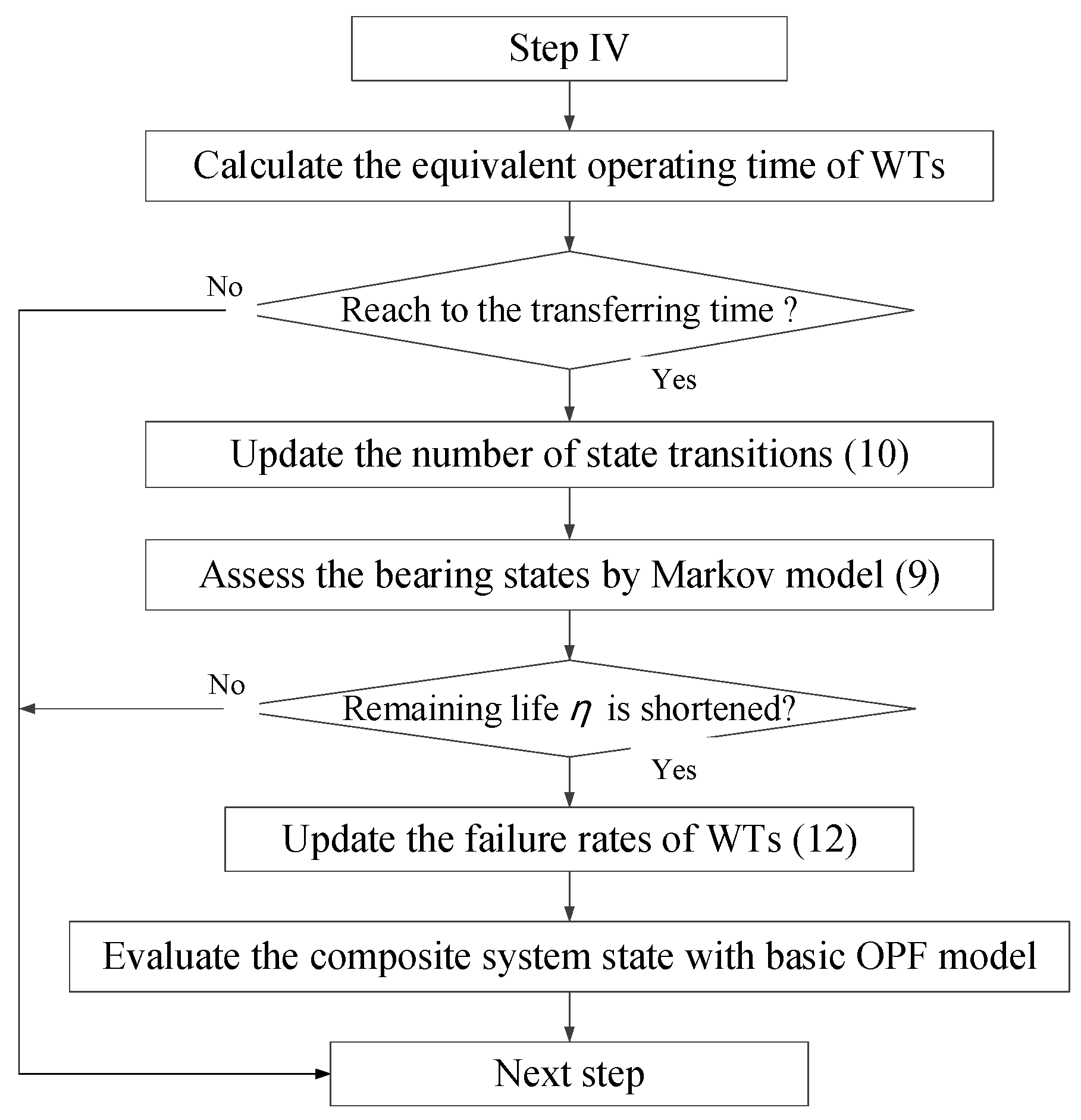
5.3. The Procedures of Reliability Assessment

Composite power system reliability assessment is based on the sequential Monte Carlo simulation. The step size of the simulation is an hour. In each step, the system states are sampled and evaluated. The power system reliability is estimated by the annual reliability indices. The flow of reliability assessment is detailed as follows:
(I) Initialize the system reliability model. Establish the basic reliability models of the power system, including the basic power flow data and the physical status of generators and transmission lines.
(II) Input the system load demand. The chronological curve of load power for 8760 h is generated. The load demand of each bus considers the characteristics of the season and workday.
(III) System states sampling. The system states contain the physical states of components, the output of WTs, and the cyber security of the wind farm. The events which deteriorate the system reliability are sampled separately. The physical failure of the components and occurrence of WPRs are sampled according to historical probability data. For a cyber-attack event, by sampling the time to compromise and defense the vulnerabilities as Equation (4), the occurrence time and frequency of cyber-attacks can be determined.
(IV) The assessment of WPRs. If WPRs exists, the ramping rates and durations are sampled by a Gaussian model. According to the ramping rate, the available power capacities of conventional generators are further updated by Equation (13). The load shedding caused by WPRs could be assessed by the basic OPF model. Then the output and the states of WTs are updated for further evaluation.
(V) The assessment of a cyber-attack. If a cyber-attack exists, the assessment consists of two typical scenarios. For the worst-case attack, the set of system active power margins shown in Equation (5) during the hidden time can be established according to the sampling results in step III. The load shedding caused by cyber-attacks is quantified by the bi-level OPF model Equations (19)–(26). For an IPA, the estimation procedure of time-varying failure rates is illustrated in Figure 4. The impact of an IPA is equivalent to the extra running time of WTs. The bearing states and their remaining life are assessed by the Markov model. When the service time and the remaining life of a WT change, the new WT failure rates should be updated with Equation (10). According to the latest failure rates, the composite system states are evaluated by the basic OPF model.
(VI) Checking the termination condition. Check if the sampling number meets the stopping criteria. If not, go back to step 2. The state sampling is conducted for 100 years.
(VII) Reliability indices calculation. When the sampling is sufficient, calculate the annual reliability indices. The reliability indices: The loss of load probability (LOLP) and expected energy not supplied (EENS) are defined as Equations (27) and (28).
L O L P = 1 N s i = 1 N s L s i
E E N S = 8760 N s i = 1 N s L p i
where NS is the total number of samples from the system state space. In the ith sample, if load curtailment occurs, Lsi equals 1; otherwise, it equals 0. Lpi is the load curtailment in the ith sample, with unit MW.

6. Case Studies and Results

The case studies were conducted on the IEEE RTS79 system [32], which has 24 buses and 38 branches. The total generating capacity of the test system was 3405 MW. The peak load was 2850 MW. Three wind farms were added, where the five 12 MW generating units on Bus 15, six 50 MW generating units on Bus 22 and the two 76 MW generators on Bus 2 were replaced by wind turbines. The penetration rate of wind power was 15%. The wind power data were from the Wind Integration National Dataset (WIND) Toolkit [33] in the New York area. With wind power generation and corresponding forecasts, the time horizon spanned from 1 January 2007 to 31 December 2012. The time resolution was 5 min. For the sake of comparative study, the CDF of the worst-case attack and the IPA followed the same Laplace distribution L (80,50).

6.1. Reliability Assessment Considering Worst-Case Attack

In the worst-case analysis, a sequential Monte Carlo simulation was conducted to estimate the system reliability indices. The load power contained the seasonal daily and hourly feature of a year. For the WPRs, the absolute value of ramping rate ranged from 133 to 2282 MW/h. The mean values of the upward and downward ramping rates were 536.5 and −494.8 MW/h, respectively. The mean ramping duration was 0.24 h. The limitation of the ramping rate in the wind farm was set as the 5% of the wind farm power capacity per minute. It was noted that when the penetration rate changed, the conventional power capacity was adjusted in proportion to keep the total install power capacity of the RTS79 system on 3405 MW.

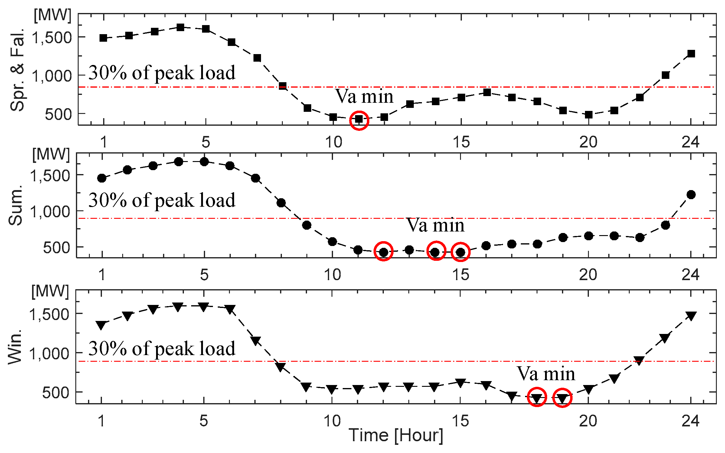
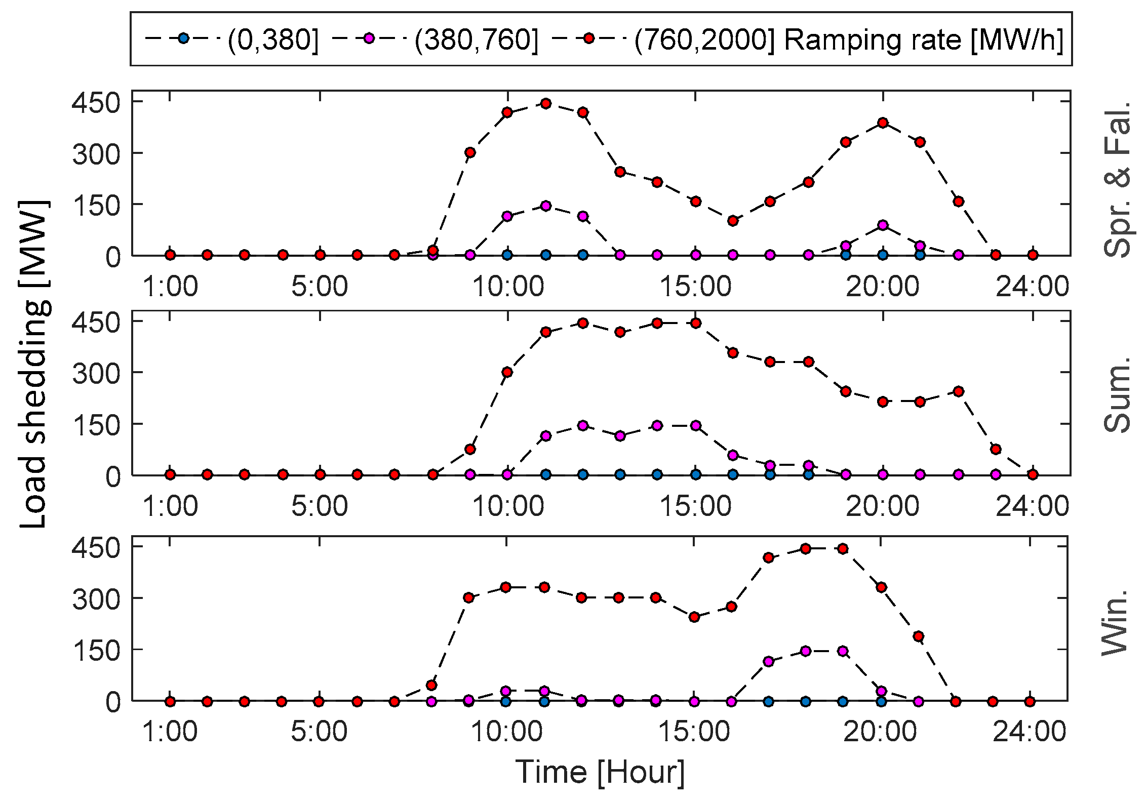
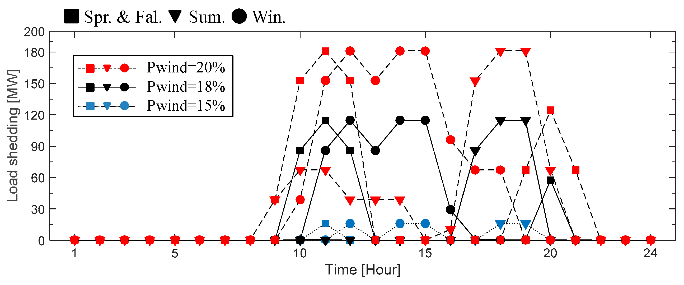
6.1.1. Impact Analysis of Worst-Case Attack

The impact of worst-case attack depends on the attack time. The system power margin varies greatly in a day. Suppose the mean output of a wind farm is 85% of its installed capacity—the seasonal and daily characteristics of the active power margin for this scenario are presented in Figure 5. As shown in the picture, from 10 a.m. to 22 p.m., the power margin is generally less than 30% of the peak load (2850 MW). Especially in summer and winter, the lowest point of the active power margin appears multiple times within a day. As such, even if the attacker does not know the accurate supply and demand relationship of the power system, the attack during the peak load may lead to a consequence close to the worst-case attack. The corresponding distribution of impact caused by an attack is shown in Figure 6. Different penetration rates are distinguished by colors, and the seasonal results are distinguished by the marked shape, which is the same in Figure 5. As shown, the load shedding caused by an attack is consistent with the change of power margin. During the period of peak load, the probability of load shedding increases greatly with the higher penetration rate.
The worst-case attack against WTs has an assignable influence on system reliability. In order to test the defense effect against cyber-attacks, four systems with different defense capabilities were evaluated by Monte Carlo simulation. The reliability result is shown in Figure 7. The system states only considered a single event of a worst-case attack. As seen in Figure 7, when the penetration rate was 15%, the EENS of the four systems from “weak” to “perfect” were 1266, 1110, 612 and 367 MWh/yr. The defense effects of the four systems became apparent with the increase of the penetration rate. For every 1% increase of the penetration rate, the EENS in a perfect system increases, on average, 316 MWh/yr. However, in a weak system, the growth of EENS reaches up to 1088 MWh/yr. Thus, a better defense ability limits the frequency of cyber-attacks and greatly improves system reliability.

6.1.2. The Composite Reliability Assessment

Based on the bi-level model, the load shedding caused by a worst-case attack can be quantified. In addition, the system states, including the different combinations of single events, were evaluated by the reliability indices as listed in Table 4. SF, SA, and SR are the single events of which the system states only contain the physical failure of components, cyber-attack and WPRs, respectively. The defense capability of the system was normal and the penetration rate of the wind power was 15%. The result shows that the EENS caused by a worst-case attack was over 1000 MWh/yr, which made the EENS twice the normal rate. Furthermore, when the system was involved with cyber-attack and WPRs, the system reliability deteriorated greatly.
Among the single events, the WPR had the greatest impact on the system reliability. The impact of WPR was close relative to the ramping rate and the available system capacity. The load shedding caused by WPRs with different load demand is presented in Figure 8. When the ramping rate was higher than 380 MW/h, during the peak load, the system available power capacity became insufficient. If the ramping rate exceeded 760 MW/h, all the wind farms were off-grid, as the dangerous ramping rate had reached the limitation and triggered the speed relay. The highest load shedding was 445 MW with a penetration rate of 15%. The EENS caused by cyber-attacks and WPRs are compared and listed in Figure 9. The growth rate of EENS caused by WPRs was slower than cyber-attacks because the system available capacity changed little as the penetration rate grew.

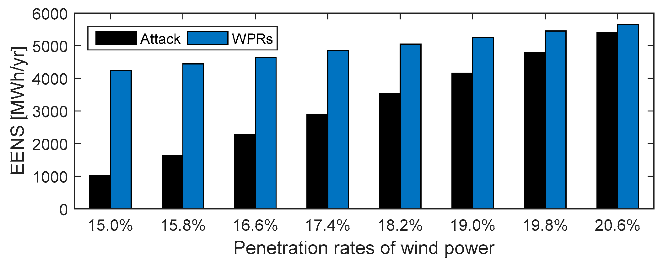
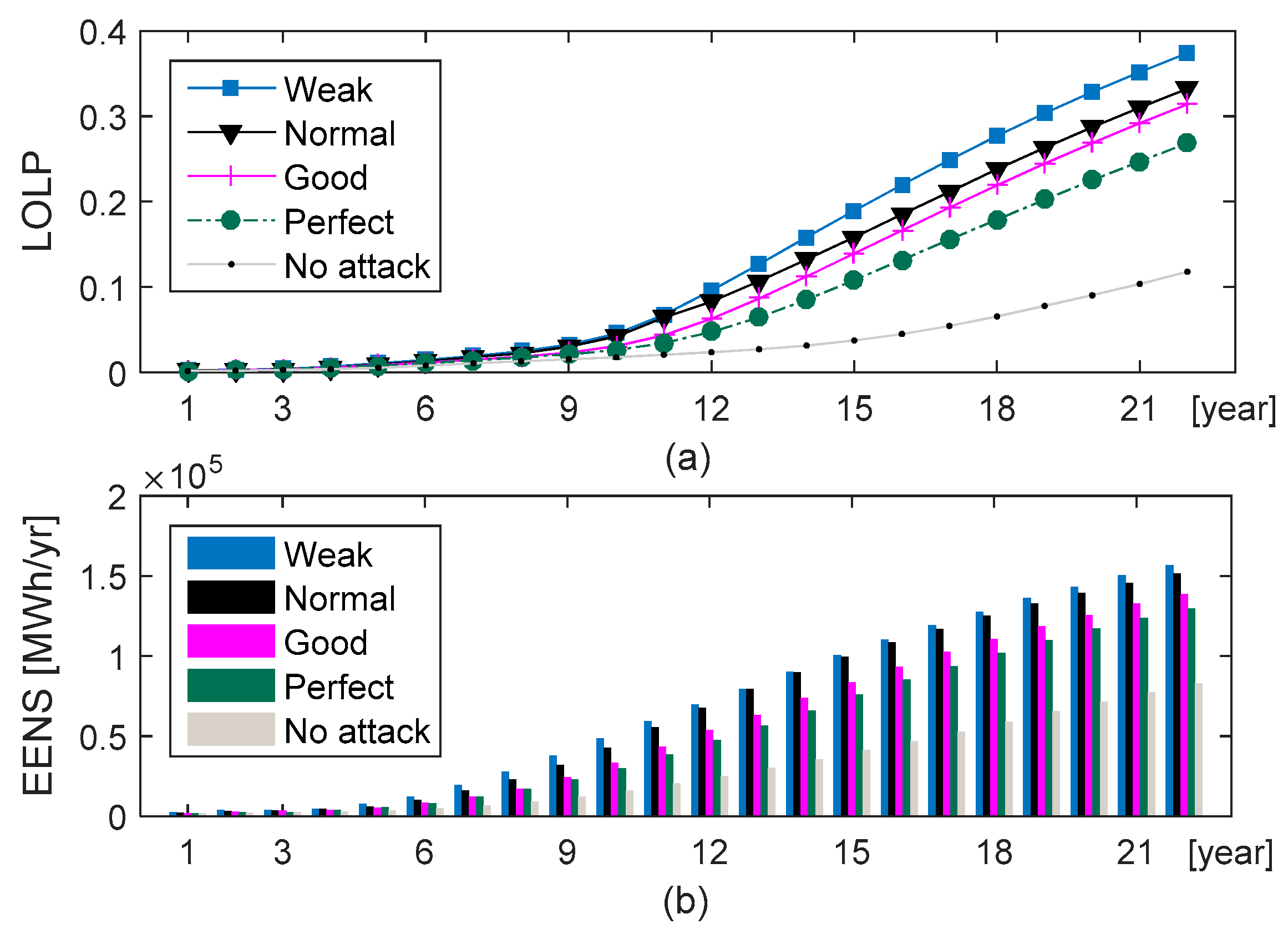
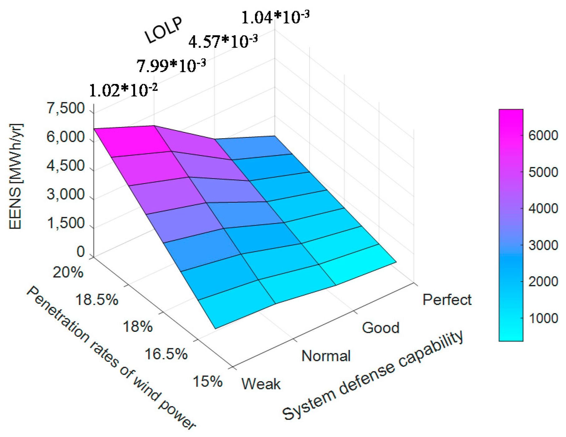
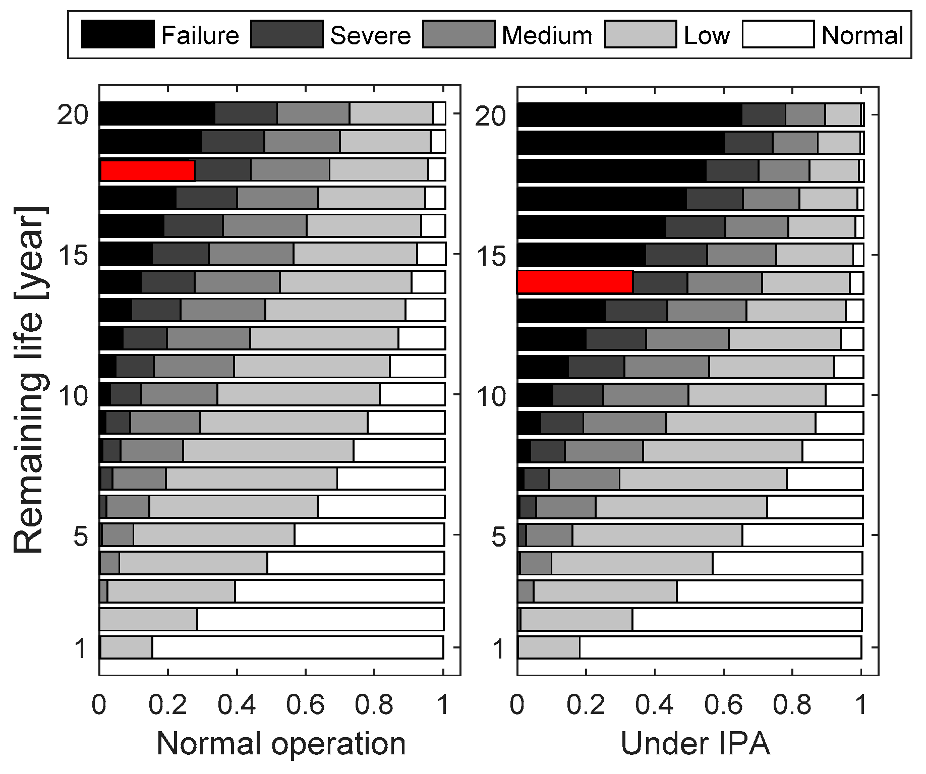
6.2. Reliability Assessment with the Imperfect Attack

An IPA directly affects the bearing of a WT. As such, in this subsection, the impacts of an IPA on the reliability of WTs and power systems are both discussed. The remaining lives of four typical bearings with and without an IPA were estimated. The rated life of bearing defined by the American Bearing Manufacturers Association (ABMA) standards was applied from the empirical data [34].
Firstly, the remaining lives of four typical bearings attacked by an IPA were tested. The remaining lives of bearings in a wind farm with a normal cyber-defense capability have been included in Table 5. SN, SL, SM and SS are the initial states of bearings as introduced in Table 2. The subscript “N” means that the bearing works under the normal condition, while the subscript “A” means it is attacked by an IPA. As the table shows, an IPA shortens bearing lives to varying degrees. In general, the remaining lives of bearings with the initial state “SN” were shortened by an average of 20%. The bearing with a better initial status was the most affected.
The probability distribution of a bearing with a rated life of 100,000 h is presented in Figure 10. Each color represents a bearing state, and the length of the block is the state probability. The left subgraph is the result that bearing works in a normal operating condition. In a normal condition, the remaining life of bearing is approximately 18 years (see the red block). After being attacked by an IPA, the failure state appeared four years earlier, as shown in the right subgraph. The duration of the normal state was decreased by 22%, and the probability of failure state also increased in the same year.
Furthermore, the remaining lives of bearings were tested in systems with different defense capabilities. As listed in Table 6, the bearings with longer rated lives were more affected. Additionally, system defense capability was important to protect the bearings. The bearing life in the system with weak defense capability could be shortened by nearly 40%. Compared to the good or perfect system, the life reduction could be controlled below 20%.
Finally, the power grid reliability considering an IPA was tested. The time-varying failure rates of WTs were modeled according to Equations (9) and (10). The rated lives of the WTs on Bus 2 and Bus 15 were set at 14 years, and the rated lives of WTs on Bus 22 were set at 18 years. Suppose all the generators are new and put into operation at the first year. If wind turbines are involved with an IPA at the first year, the system reliability results within 22 years are presented in Figure 11.
The reliability indices show that the power system suffered a huge power loss in the later stage. Since the IPA reduced the rated WT life, as seen in Table 6, the reliability indices of systems attacked had a rapid growth over time from the 10th year. As shown in Figure 11, there was an obvious gap between the systems with and without being attacked. Especially the weak system, its LOLP reached 0.1 in the 12th year. In comparison, although the WTs had exceeded their rated lives at 18th year, the LOLP of the system without being attacked was far below 0.1.

7. Conclusions

This paper developed a power system reliability evaluation method which considers the cybersecurity and WPRs of a wind farm. It is concluded that: (i) The instant worst-case attack and long termed imperfect attack lead to non-negligible consequence to the power system in different time scales. The cybersecurity of a wind farm has a great influence on power system reliability. (ii) The failure rate of a wind turbine attacked by an IPA grows rapidly, and its remaining life is shortened by nearly 20%. (iii) The period of peak load is the vulnerable time of power system. The system reliability will benefit from the re-dispatching of power reserves with a reasonable ramping rate, which reduces both the impact of cyber-attacks and WPRs.
Periodic vulnerabilities patching and intrusion detection are of great importance for cybersecurity. To better estimate the frequency of cyber-attacks, the stochastic attack–defense model can be further improved by using the statistics from the common vulnerability scoring system [21]. Combined with firewalls, encryption, system hardening, and physical security, wind farm owners should pay more attention to the operation states of wind turbines. Equipment operating in critical conditions should be monitored in a timely manner. In future work, a dynamic analysis and detection of an IPA will be further studied.

Author Contributions

Conceptualization, H.W. and J.L. (Junyong Liu); methodology, H.W.; software, M.C.; validation, H.W., J.L. (Jichun Liu) and X.L.; formal analysis, H.W.; investigation, H.G.; resources, M.C.; data curation, J.L. (Junyong Liu); writing—original draft preparation, H.W.; writing—review and editing, M.C.; visualization, X.L.; supervision, J.L. (Junyong Liu); project administration, J.L. (Junyong Liu); funding acquisition, J.L. (Jichun Liu).

Funding

This research was founded by China national key research and development program, grant number 2018YFB0905200.

Conflicts of Interest

The authors declare no conflict of interest.

References

  1. GLOBAL STATUS OVERVIEW GWEC. Available online: https://gwec.net/global-figures/wind-energy-global-status/ (accessed on 17 February 2019).
  2. Lai, J.; Duan, B.; Su, Y.; Li, L.; Yin, Q. An active security defense strategy for wind farm based on automated decision. In Proceedings of the 2017 IEEE Power Energy Society General Meeting, Chicago, IL, USA, 16–20 July 2017; pp. 1–5. [Google Scholar]
  3. Falahati, B.; Kahrobaee, S.; Ziaee, O.; Gharghabi, P. Evaluating the differences between direct and indirect interdependencies and their impact on reliability in cyber-power networks. In Proceedings of the 2017 IEEE Conference on Technologies for Sustainability (SusTech), Phoenix, AZ, USA, 12–14 November 2017; pp. 1–6. [Google Scholar]
  4. Han, Y.; Wen, Y.; Guo, C.; Huang, H. Incorporating Cyber Layer Failures in Composite Power System Reliability Evaluations. Energies 2015, 8, 9064–9086. [Google Scholar] [CrossRef] [Green Version]
  5. Huang, L.; Fu, Y.; Mi, Y.; Cao, J.; Wang, P. A Markov-Chain-Based Availability Model of Offshore Wind Turbine Considering Accessibility Problems. IEEE Trans. Sustain. Energy 2017, 8, 1592–1600. [Google Scholar] [CrossRef]
  6. Mitchell, R.; Chen, I. Modeling and Analysis of Attacks and Counter Defense Mechanisms for Cyber Physical Systems. IEEE Trans. Reliab. 2016, 65, 350–358. [Google Scholar] [CrossRef]
  7. Zhang, Y.; Wang, L.; Xiang, Y.; Ten, C.W. Power System Reliability Evaluation with SCADA Cybersecurity Considerations. IEEE Trans. Smart Grid 2015, 6, 1707–1721. [Google Scholar] [CrossRef]
  8. Chen, Y.; Li, Y.; Li, W.; Wu, X.; Cai, Y.; Cao, Y.; Rehtanz, C. Cascading Failure Analysis of Cyber Physical Power System with Multiple Interdependency and Control Threshold. IEEE Access 2018, 6, 39353–39362. [Google Scholar] [CrossRef]
  9. Kateb, R.; Tushar, M.H.K.; Assi, C.; Debbabi, M. Optimal Tree Construction Model for Cyber-Attacks to Wide Area Measurement Systems. IEEE Trans. Smart Grid 2018, 9, 25–34. [Google Scholar] [CrossRef]
  10. Zhang, Y.; Wang, L.; Sun, W. A preliminary study of power system reliability evaluation considering cyber attack effects. In Proceedings of the 2013 IEEE Power Energy Society General Meeting, Vancouver, BC, Canada, 21–25 July 2013; pp. 1–5. [Google Scholar]
  11. Johnson, P.; Lagerstrom, R.; Ekstedt, M.; Franke, U. Can the Common Vulnerability Scoring System be Trusted? A Bayesian Analysis. IEEE Trans. Dependable Secur. Comput. 2016, 15, 1002–1015. [Google Scholar] [CrossRef]
  12. Nzoukou, W.; Wang, L.; Jajodia, S.; Singhal, A. A Unified Framework for Measuring a Network’s Mean Time-to-Compromise. In Proceedings of the 2013 IEEE 32nd International Symposium on Reliable Distributed Systems, Braga, Portugal, 30 September–3 October 2013; pp. 215–224. [Google Scholar]
  13. Kapourchali, M.H.; Sepehry, M.; Aravinthan, V. Fault Detector and Switch Placement in Cyber-Enabled Power Distribution Network. IEEE Trans. Smart Grid 2018, 9, 980–992. [Google Scholar] [CrossRef]
  14. Staggs, J.; Ferlemann, D.; Shenoi, S. Wind farm security: Attack surface, targets, scenarios and mitigation. Int. J. Crit. Infrastruct. Prot. 2017, 17, 3–14. [Google Scholar] [CrossRef]
  15. Yan, J.; Liu, C.C.; Govindarasu, M. Cyber intrusion of wind farm SCADA system and its impact analysis. In Proceedings of the 2011 IEEE/PES Power Systems Conference and Exposition, Phoenix, AZ, USA, 20–23 March 2011; pp. 1–6. [Google Scholar]
  16. Zhang, Y.; Xiang, Y.; Wang, L. Power System Reliability Assessment Incorporating Cyber Attacks Against Wind Farm Energy Management Systems. IEEE Trans. Smart Grid 2017, 8, 2343–2357. [Google Scholar] [CrossRef]
  17. Cui, M.; Feng, C.; Wang, Z.; Zhang, J. Statistical Representation of Wind Power Ramps Using a Generalized Gaussian Mixture Model. IEEE Trans. Sustain. Energy 2018, 9, 261–272. [Google Scholar] [CrossRef]
  18. Qi, Y. Wind Power Ramping Control Using Competitive Game. IEEE Trans. Sustain. Energy 2016, 7, 9. [Google Scholar] [CrossRef]
  19. Gong, Y.; Chung, C.Y.; Mall, R.S. Power System Operational Adequacy Evaluation with Wind Power Ramp Limits. IEEE Trans. Power Syst. 2018, 33, 2706–2716. [Google Scholar] [CrossRef]
  20. Mohammadpourfard, M.; Sami, A.; Weng, Y. Identification of False Data Injection Attacks with Considering the Impact of Wind Generation and Topology Reconfigurations. IEEE Trans. Sustain. Energy 2017, 9, 1349–1364. [Google Scholar] [CrossRef]
  21. Mell, P.; Scarfone, K.; Romanosky, S. Common Vulnerability Scoring System. IEEE Secur. Priv. 2006, 4, 85–89. [Google Scholar] [CrossRef]
  22. Jonsson, E. A Quantitative Model of the Security Intrusion Process Based on Attacker Behavior. IEEE Trans. Softw. Eng. 1997, 23, 235–245. [Google Scholar] [CrossRef]
  23. Ghirmai, T. Laplace Autoregressive Model for Cascaded Systems. IEEE Trans. Syst. Man Cybern. Syst. 2016, 46, 771–781. [Google Scholar] [CrossRef]
  24. Verizon. 2017 Data Breach Investigations Report, Verizon Enterprise Solutions, Investigations Report; Verizon: New York, NY, USA, 2017; p. 10. [Google Scholar]
  25. Falliere, N.; Murchu, L.; Chien, E. W32.Stuxnet Dossier. Symantec Secur. Response 2011, 5, 1–68. [Google Scholar]
  26. Ribrant, J.; Bertling, L.M. Survey of Failures in Wind Power Systems with Focus on Swedish Wind Power Plants During 1997–2005. IEEE Trans. Energy Convers. 2007, 22, 167–173. [Google Scholar] [CrossRef]
  27. Tautz-Weinert, J.; Watson, S.J. Using SCADA data for wind turbine condition monitoring a review. IET Renew. Power Gener. 2017, 11, 382–394. [Google Scholar] [CrossRef]
  28. Wysoclci, A.; Feest, B. Bearing Failure: Causes and Cures; ECM Electrical Construction Maintenance: Perth, Australia, 1997. [Google Scholar]
  29. Nguyen, K.T.P.; Fouladirad, M.; Grall, A. New Methodology for Improving the Inspection Policies for Degradation Model Selection According to Prognostic Measures. IEEE Trans. Reliab. 2018, 67, 1269–1280. [Google Scholar] [CrossRef] [Green Version]
  30. Sumereder, C. Stat. lifetime of hydro generators and failure analysis. IEEE Transactions Dielectr. Electr. Insul. 2008, 15, 678–685. [Google Scholar] [CrossRef]
  31. Cui, M.; Zhang, J.; Florita, A.R.; Hodge, B.; Ke, D.; Sun, Y. An Optimized Swinging Door Algorithm for Identifying Wind Ramping Events. IEEE Trans. Sustain. Energy 2016, 7, 150–162. [Google Scholar] [CrossRef]
  32. Subcommittee, P.M. IEEE Reliability Test System. IEEE Trans. Power Appar. Syst. 1979, PAS-98, 2047–2054. [Google Scholar] [CrossRef]
  33. Draxl, C.; Clifton, A.; Hodge, B.M.; McCaa, J. The Wind Integration National Dataset (WIND) Toolkit. Appl. Energy 2015, 151, 355–366. [Google Scholar] [CrossRef] [Green Version]
  34. Bearings for Wind Turbines. Available online: https://anagnostou-sa.gr/wp-content/uploads/2017/06/URB-Wind-Bearings.pdf (accessed on 9 August 2018).
Figure 1. The supervisory control and data acquisition (SCADA) network in a wind farm.
Applsci 09 03003 g001
Figure 2. Typical time relationship of attacking capacity.
Applsci 09 03003 g002
Figure 3. The performance of vulnerability fixing in a typical system.
Applsci 09 03003 g003
Figure 4. The flow of estimating the time-varying failure rates of wind turbines (WTs).
Applsci 09 03003 g004
Figure 5. The time distribution of active power margin.
Applsci 09 03003 g005
Figure 6. The time distribution of load shedding.
Applsci 09 03003 g006
Figure 7. Reliability performances of systems with different defense capabilities.
Applsci 09 03003 g007
Figure 8. Distribution of load shedding caused by wind power ramping events (WPRs).
Applsci 09 03003 g008
Figure 9. EENS caused by cyber-attacks and WPRs.
Applsci 09 03003 g009
Figure 10. Probability distribution of bearing state.
Applsci 09 03003 g010
Figure 11. Reliability indices of system attacked by an imperfect attack (IPA). (a) LOLP; (b) EENS.
Applsci 09 03003 g011
Table 1. Defense parameters of different systems.
Defense Capabilityα0α1α2β
Weak000.20.8
Normal00.20.20.6
Good0.20.30.40.1
Perfect0.70.20.10
t1 = 7, t2 = 28, t3 = 84.
Table 2. Probabilities of a cyber-attack.
DC0 < t ≤ 77 < t ≤ 2828 < t ≤ 8484 < t ≤ 365PM
Weak0.2450.0880.2350.2540.010
Normal0.2450.0700.1760.1900.008
Good0.0200.0440.0290.0320.004
Perfect0.0070.088000.001
DC is the defense capability of power system, and PM is the annual mean probability of a cyber-attack.
Table 3. Wearing conditions of bearing.
Bearing ConditionsWear Interval
SN: Normal(0~0.2) Δmax
SL: Low(0.2~0.4) Δmax
SM: Medium(0.4~0.7) Δmax
SS: Severe(0.7~1.0) Δmax
SF: Failure>Δmax
Table 4. Reliability result of different system states.
No.EventLOLPEENS [MWh/yr]
1SF4.09 × 10−31.68 × 10+3
2SA7.99 × 10−31.11 × 10+3
3SR3.20 × 10−34.04 × 10+3
4SR∪SA3.28 × 10−36.08 × 10+3
5SA∪SF4.72 × 10−33.50 × 10+3
6SR∪SF5.57 × 10−39.02 × 10+3
7SR∪SA∪SF9.02 × 10−31.17 × 10+4
Penetration rate of wind power is 15%.
Table 5. Remaining lives of bearings in different states [year].
Rated Life [h]SNSLSMSS
NANANANA
30,0005433220.20.2
60,00011976440.40.4
80,000141198550.60.4
100,00018141210660.60.6
Table 6. Remaining lives of bearings in different system [year].
Rated Life [h]No AttackPerfectGoodNormalWeak
30,00055443
60,0001110997
80,000141212119
100,0001816151411

