High-Speed Railway Clearance Intrusion Detection with Improved SSD Network

Featured Application

This work can be widely used in high-speed railway clearance intrusion detection with image object classification and recognition.

Abstract

With the rapid development of high-speed railways, any objects intruding railway clearance will do great threat to railway operations. Accurate and effective intrusion detection is very important. An original Single Shot multibox Detector (SSD) can be used to detect intruding objects except small ones. In this paper, high-level features are deconvolved to low-level and fused with original low-level features to enhance their semantic information. By this way, the mean average precision (mAP) of the improved SSD algorithm is increased. In order to decrease the parameters of the improved SSD network, the L1 norm of convolution kernel is used to prune the network. Under this criterion, both the model size and calculation load are greatly reduced within the permitted precision loss. Experiments show that the mAP of our method on PASCAL VOC public dataset and our railway datasets have increased by 2.52% and 4.74% respectively, when compared to the original SSD. With our method, the elapsed time of each frame is only 31 ms on GeForce GTX1060.

1. Introduction

As of 2018, the length of high-speed railway lines in China had exceeded 29,000 km. With the increasing of speed, any object intruding railway clearance will pose a major threat to high-speed trains. Effective intrusion detection methods are of great significance to the safety of a high-speed railway operation. Machine vision is an effective non-contact intrusion detection method widely used in railways for the advantage of easy maintenance and intuitive results. Most of these methods detect intruding objects with background subtraction [1]. The disturbance of strong environment light and severe weather will lead to false alarms. To solve this problem, the convolutional neural network (CNN) [2] was used to detect objects intruding railway clearance. CNN has a good rotation and translation invariance, which can effectively reduce the impact of camera shake and light changing. Moreover, CNN has developed rapidly in recent years. From Lenet-5 [3] to Alexnet [4], VGGNe [5], GoogLeNet [6] and ResNet [7], the depth of the CNN network has reached hundreds of layers, and the recognition effect has gradually improved. However, all these networks are classification models. They need to be retrained when the scene changes because of their weak generalization ability. They are ineffective in railway clearance intrusion detection. Therefore, it is of great significance to have a novel CNN network which can detect objects in railway images.

At present, object detection methods with CNN are mainly divided into two types. One is based on regional candidate models (such as R-CNN, Fast R-CNN and Faster R-CNN), the other is based on regression models (such as YOLO and SSD). In 2014, Girshick [8] proposed the R-CNN model, which extracted candidate regions with a selective search method, extracted candidate region features with CNN, and classified candidate box regions with SVM. But the speed and accuracy were slow. To solve the problem, a Fast R-CNN model [9] was also proposed by Girshick in 2015. A box regression algorithm was directly added to the CNN network for training with a multi-task loss function. The mean average precision (mAP) is higher than R-CNN but not fast enough for real-time detection. Ren [10] proposed the Faster-Rcnn model, which used the Region Proposal Network (RPN) to predict the bounding box directly. The recognition time was reduced to 198 ms, since most of the prediction was completed in GPU. In 2016, Redmon [11] proposed the YOLO model, which greatly speeded up the detection speed by directly detecting the last feature map in CNN. However, the bounding box location error of YOLO was large. Liu [12] extracted bounding boxes from CNN multi-layer feature maps to improve the speed and accuracy with the SSD model. Among the above algorithms, the SSD model has a higher speed and accuracy. The mAP on the PASCAL VOC 2007 dataset was 74.3%, and the elapsed time was only 36.2 ms in GeForce GTX1060. However, the detection performance of SSD for small objects is unsatisfactory, and the effect directly used in railway clearance intrusion detection is poor.

In order to solve this problem, this paper proposes an improved SSD method for railway clearance intrusion detection. The SSD is improved on the basis of the DeepLab network structure [13]. High-level features are deconvolved to low-level and fused with original low-level features to enhance their semantic information and improve the detection accuracy. In order to reduce the model parameters and calculation load within a permitted loss of accuracy, the unimportant weights in the network are pruned with the L1 norm criterion [14].

Our main contributions are as follows:

-

The deconvolution structure is introduced into the SSD network to improve the detection ability of small objects. 19 × 19 and 38 × 38 feature maps are deconvolved to and fused with 38 × 38 and 75 × 75 feature maps, respectively.

-

A recursive SSD network pruning method is proposed to reduce the model parameters and calculation load with the convolution kernel L1 norm criterion within a 1% precision loss.

-

Compared with original SSD, the recognition speed and accuracy of our method both improved. The mAP of our method on PASCAL VOC and railway datasets increased by 2.52% and 4.74%. The elapsed times of a single image are 35.5 ms and 31.0 ms, respectively.

The remainder of this paper is organized as follows: Related works are addressed in Section 2. An improved SSD network with a deconvolution structure is proposed in Section 3. Section 4 introduces the details of network pruning with the L1 norm criterion. The experimental results and the performance analysis are discussed in Section 5. Section 6 draws conclusions and indicates lines of future research work.

2. Related Works

2.1. Related Works of Railway Clearance Intrusion Detection

At present, many studies focus on railway clearance intrusion detection methods. Garcia et al. [15] proposed a multi-sensor system for the detection of obstacles. The system consists of emitting and receiving barriers placed on opposing sides of the railway. Infrared and ultrasonic sensors are used to establish optical and acoustic links between them. Punekar et al. [16] proposed a train location method with GPS and GSM, which helped to track trains and provided their position information to avoid accidents. Catalano et al. [17] used fiber Bragg grating sensors to detect the intrusion of railway objects. These methods are easily disturbed by environmental factors such as the weather and vibrations. With the development of machine vision technology, clearance intrusion detection with image processing has been widely used in railways. Sriwardene et al. [18] proposed a smart driver assisting system, which could detect obstacles in the rail area. Nakasone et al. [19] proposed a railway intrusion detection algorithm using a monocular camera and background subtraction. An image processing method including subtraction, binarization, morphological transformation and segmentation was used to track down moving obstacles at the level crossing [20]. A novel registration and fusion algorithm for multimodal railway images with different fields of views to detect objects was proposed by Guo and Zhou [21]. Tastimur et al. [22] proposed an onboard objects detection method at intersection areas. However, all these traditional methods are based on background subtraction. Due to the difficulty in real-time background updating, the detection effect is very poor, especially when the camera is shaking and there are sudden illumination changes. Because of their good rotation and translation invariance, CNN can be used for objects detection in complex railway environments.

2.2. Object Detection with CNNs

Before CNN, some machine learning algorithms had been applied to object detection. Viola et al. [23] used the AdaBoost algorithm to select Haar features for face detection at 67 ms for a face image, but the resolution of the face detection dataset is only 24 × 24. However, the resolution of pedestrians and trains in the railway dataset ranges from 50 × 70 to 800 × 600. Haar features, using this method, will take a lot of time and cannot meet the real-time requirements in the railway field. HOG was used to extract features, and SVM was used to detect pedestrians by Dalal [24]. Chen et al. [25] presented a novel model that utilized both sparsity and low-rankness with contextual regularization to detect moving objects in multi scenario surveillance data. These methods are effective in the case of small background changing. However, the detection effect is poor with large background changing. CNN can deal with the situation of large background changing and is suitable for the detection of continuous frames with a dynamic background. Temesguen et al. [26] combined a KNN classifier with a deep learning method to classify malware. However, it is not enough to classify the images on the railway dataset. There are two stages in the early CNN object detection method. Candidate boxes were firstly extracted by a selective search algorithm [27,28], after which the object location and classification were completed by the CNN network. RCNN [8], SPPNet [29] and Fast-RCNN [9] all constitute these methods. Faster-RCNN [10] greatly improves the training and detection speed of the RPN network instead of a selective search algorithm. However, the calculation load and parameters of the two-stage target detection algorithm are still too large for real-time detection. Therefore, one-stage, end-to-end target detection algorithms, such as Overfeat [30], YOLO [11] and SSD [12], were proposed. They can extract, locate and classify bounding boxes directly by convolution, which greatly improves the speed of the target detection. Lin et al. [31] proposed focal loss to address the foreground-background class imbalance to improve the objects detection accuracy. Fu et al. [32] proposed the DSSD model by replacing the pre-network in SSD with Resnet-101. The detection accuracy of DSSD was greatly improved, but the complexity and elapsed time were also greatly increased. The object detection CNN network has been widely used in transportation. Amato et al. [33] proposed mLenet and mAlexnet structures for parking spaces statistics, but they only available in good weather condition. Wang et al. [34] completed different vehicle type identifications by introducing a maximum mean discrepancy into a migration learning task based on CNN. Hu et al. [35] combined traditional CNN with a spatial pyramid strategy to recognize the vehicle color under various conditions, but the accuracy was poor at night. Ye et al. [36] proposed a CNN-based railway object detection network consisting of three connected modules, i.e., a depthwise-pointwise convolution module, coarse detection module and object detection module. Railway experiments showed that the network could distinguish straight, railway left, right, pedestrian, bullet train, and safety helmets. All these objects in this paper were not far from cameras and were easy to recognize. There are so many cameras along high-speed railway lines that we need a more efficient network structure. Mobilenet [37] uses deep separable convolution to reduce model parameters. Squeezenet [38] reduces parameters by replacing the 3 × 3 convolution kernel with the 1 × 1 convolution kernel in the network. Courbariaux et al. [39] proposed a compressed model to reduce the parameters by binarizing the weights. Han et al. [40] accomplished network compression through pruning, trained quantization and huffman coding.

In this paper, in order to achieve the balance of recognition accuracy and speed, a deconvolution structure is added to SSD. In order to reduce the calculation load and parameters, the convolution kernel L1 norm is used to prune the unimportant weights in the network and speed up the detection process.

3. Improved SSD Network Structure

3.1. SSD Network Analysis

SSD is a one-stage object detection network, as shown in Figure 1. The pre-convolution network is used to extract image features by adding six convolution layers after the VGG16 network. Then, the bounding boxes of different scales, with their category and location, are extracted on the six-layer feature maps. The bounding box locations are amended with a regression procedure [12] and refined with a non-maximum suppression algorithm. Therefore, the training of SSD regresses both the object locations and types. The loss function includes two parts: confidence loss and location loss, as shown in Formula (1).

$$L(z,c,l,g)=\frac{1}{N}(L_{conf}(z,c)+\alpha L_{loc}(z,l,g))$$

(1)

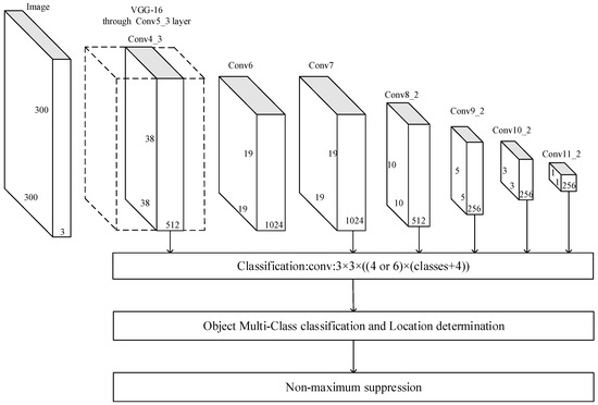
Figure 1. Single Shot multibox Detector (SSD) network structure.

In Formula (1), N is the number of matched default boxes; $L_{conf}(z,c)$ is the confidence loss function; The location loss function $L_{loc}(z,l,g))$ is Smooth L1 loss [12]; z is the matching result of the default box and the ground truth box of different kinds of objects; c is the confidence of the predicting box; l is the position of the predicting box, g is the position of the ground truth box; $\alpha$ is the parameter to balance the confidence loss and location loss, which is generally set to 1. By reducing the value of the loss function in the training process, the class confidence and position accuracy of the predicting box can be improved.

As shown in Figure 1, SSD extracts default boxes from each unit of Conv4_3, Conv7, Conv8_2, Conv9_2, Conv10_2 and Conv11_2. The regression procedure of Formula (1) in the training stage will make the default boxes as close as possible to the ground truth boxes. The resolution of six convolution layers decreases from the front to back, but their corresponding feature level increases. For instance, the Conv4_3 layer has the highest resolution of 38 × 38, but its corresponding feature is the lowest level; and the Conv11_2 layer has the lowest resolution of 1 × 1, but its corresponding feature is the highest level. In the test phase, each default box is matched with the ground truth box and reduced by a non-maximum suppression algorithm. Conv4_3 has the highest resolution in the six convolution layers and contains more details of small objects. However, the details are not enough for small objects detection. This will lead to a significant increase in the calculation load and an over-fitting of high-level feature maps if convolution layers are added before this layer. For an original image in Figure 2a, the low-level and high-level feature maps are shown in Figure 2b,c.

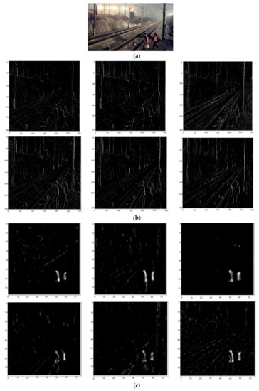
Figure 2. Feature maps of different feature layers. (a) Original Image. (b) Low-level feature map. (c) High-level feature map

From Figure 2, we can see that low-level feature maps have better edge information, and high-level feature maps have stronger semantic information. In order to improve the small object detection ability, feature maps should not only have a high resolution to detect small objects, but also have stronger semantic information to detect the location and category information.

3.2. Improved SSD with Deconvolution

Deconvolution is the inverse process of convolution. High-level features are mapped to low-level features by deconvolution to enrich their semantic information. The deconvolution schematic is shown in Figure 3.

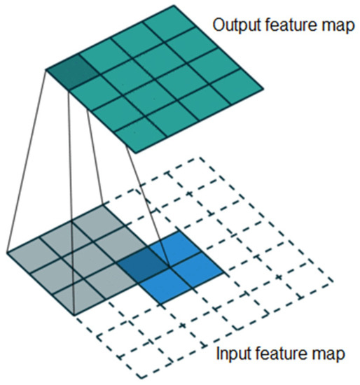
Figure 3. Schematic diagram of deconvolution.

The deconvolution operation is completed with the matrix multiplication of a one-dimensional vector expanding from the feature map and a sparse matrix expanding from the convolution kernel. The deconvolution calculation is shown in Formula (2):

$$C^{\mathrm{T}}\ast \overrightarrow{X}=\overrightarrow{Y}$$

(2)

where $\overrightarrow{X}$ and $\overrightarrow{Y}$ represent one-dimensional vectors expanded from the input and output features. C denotes the sparse matrix by expanding the convolution kernel. Deconvolution is an inverse process of normal forward propagation of convolution only by exchanging the input and output feature maps. Therefore, the parameters of the deconvolution kernel are the same as those of the convolution kernel. In the training process, the parameters of the deconvolution kernel can be learned by a back propagation algorithm.

Through deconvolution, high-level features can be mapped onto low-level features. The new features are spliced with the original low-level features to achieve a feature fusion. The default boxes are extracted from the combined feature maps. The low-level feature map will have more global information by combining with the mapping feature without changing the fitting ability of the high-level feature map. The feature fusion method with deconvolution is shown in Figure 4.

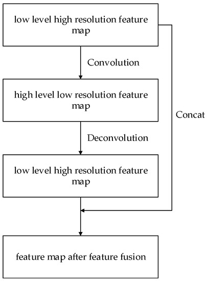
Figure 4. Feature fusion with deconvolution.

In order to improve the SSD detection ability of small objects without increasing too much computation, we introduce deconvolution only to low levels, since they contain more details of small objects.

The input image is 300 × 300. A feature map with a resolution of 75 × 75 is added as a detection layer. Feature maps with resolutions of 19 × 19 and 38 × 38 are deconvoluted and fused with 38 × 38 and 75 × 75 feature maps. The resolution relationship between the deconvolution input and output feature maps is shown as Equation (3):

$$O=S\times (W-1)+F-2\times P$$

(3)

where O is the resolution of the output feature map; S is the stride of the convolution kernel, W denotes the resolution of the input feature map; F is the convolution kernel size; and P is the padding size. In order to splice, it is necessary to ensure that the resolution of the deconvolution feature maps is consistent with that of the low-level feature maps. In Formula (3), the deconvolution kernel size of the 19 × 19 feature maps is 2 × 2, stride is 2, and padding size is 0. The deconvolution kernel size of the 38 × 38 feature maps is 3 × 3, stride is 2, and padding size is 1.

The structure of the improved SSD network is shown in Figure 5. Conv3_3 and Conv5_3 are used as detection layers. The feature map sizes of Conv3_3, Conv4_3, and Conv5_3 are 75 × 75, 38 × 38, and 19 × 19, respectively. The feature map DeConv5_3 is deconvoluted by Conv5_3 with a resolution of 38 × 38 and spliced to Conv4_3 for the feature fusion. The fused feature map is named Feature Fusion 1 (FF1). The feature map DeConv4_3 is deconvoluted by Conv4_3 with a resolution of 75 × 75 and spliced to Conv3_3 for the feature fusion. The fused feature map is named Feature Fusion 2 (FF2).

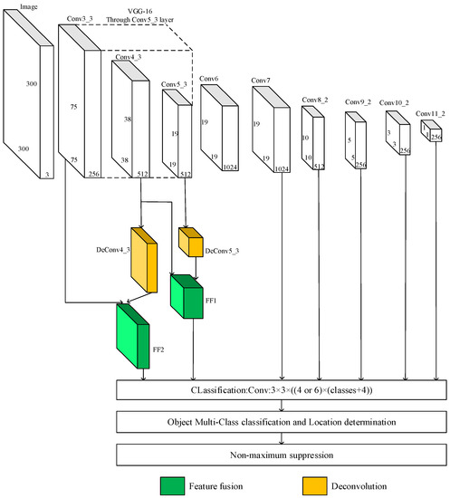
Figure 5. Improved SSD network. FF2, FF1, Conv7, Conv8_2, Conv9_2, Conv10_2 and Conv11_2 are used to extract the default boxes. By deconvolution and feature fusion, the detection ability of the SSD network for small objects is improved.

4. Network Model Pruning with L1 Norm Criterion

Improved SSD with deconvolution can improve the ability of small objects detection. However, there is a sharp increase of the network model size and calculation load. The network model size can be decreased with weight parameters pruning. In this paper, the SSD network is pruned with the L1 norm criterion of the convolution kernels. The pruned network weights are used as initial parameters for fine tuning. Through this, the model size and calculation load of the improved SSD network can be greatly reduced without an obvious loss of accuracy.

The convolution operation can be expressed as Equation (4):

$$g(i,j)={\displaystyle \sum _{k,l}f(i+k,j+l)h(k,l)}$$

(4)

where g(i,j) is the value of each pixel in the output feature map; f(i + k,j + l) is each pixel value in the input feature map; and h(k,l) is the convolution kernel value. When the convolution kernel slides over the whole image, the image convolution is essentially the sum of the product of the convolution kernel and the corresponding pixels of the coverage area. In this paper, L₁(F_j) is the L1 norm of each convolution kernel F_j. It is considered that the convolution kernels with a smaller L1 norm have less influence on the network model and belong to redundant convolution kernels. The convolution kernels with a smaller L1 norm are pruned after sorting all L1 norms of each convolution kernel. The pruned network is retrained to ensure its accuracy. The L1 norm of the convolution kernel can be defined as Formula (5):

$$L_1(F_j)={\displaystyle \sum _{i=1}^{n_k}({\displaystyle \sum _{s\times s}\left|F_j\right|})}$$

(5)

where F_j denotes the jth convolution kernel, s is the size of the convolution kernel, n_k denotes the dimension of the convolution kernels, and L₁(F_j) is the L1 norm of F_j. The process of pruning using the L1 norm criterion is shown in Figure 6. The original network is shown in Figure 6a. The input feature map H₀ with M₀ channels is convoluted with the M₁ convolution kernels to generate the feature map H₁ with M₁ channels. The feature map H₁ with M₁ channels is convoluted with the M₂ convolution kernels to generate the feature map H₂ with M₂ channels. The pruning process of the network structure is shown in Figure 6b.

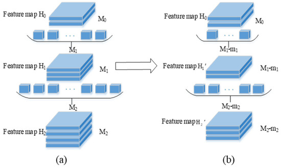
Figure 6. Pruning network model. (a) Before pruning. (b) After Pruning.

In the first convolution level, the m₁ convolution kernels are removed from M₁ by the L1 norm criterion. The input feature map H₀ with M₀ channels is convoluted with the (M₁-m₁) convolution kernels to generate the feature map H₁’ with (M₁-m₁) channels.

In the second convolution level, the m₂ convolution kernels are removed from the M₂ kernels. The feature map H₁’ with (M₁-m₁) channels is convoluted with the (M₂-m₂) convolution kernels to generate the feature map H₂’ with (M₂-m₂) channels.

The procedure of the improved SSD network pruning is as follows:

(1)

For each layer, the L1 norm of each convolution kernel is sorted from small to large. The convolution kernels with a smaller L1 norm are pruned. After pruning, the channels of the feature map will be reduced. Therefore, the convolution kernels of the next level should also be pruned.

(2)

The pruned network weight is used as an initial parameter for fine-tuning. During the fine-tuning phase, the pre-VGG network structure is firstly frozen. The convolution layers after VGG are fine-tuned until their accuracy is stable. Then, the pre-VGG network is fine-tuned. This method can reduce the loss of network accuracy as much as possible.

(3)

Repeat the prior two steps for recursive pruning until the precision loss is larger than a preset threshold.

Through this, the model parameters and computation are both reduced.

5. Experimental Section and Results

In order to verify the effectiveness of our method, experiments were carried out on PASCAL VOC and high-speed railway datasets. For a better robustness, besides the original image samples of the dataset, one of the following two ways was used for data augmentation:

(1)

Sample a patch so that the minimum jaccard overlap with the objects is 0.1, 0.3, 0.5, 0.7, or 0.9.

(2)

Randomly sample a patch.

After the training dataset is expanded by the above methods, the training samples are more diverse and increased by 2 times. The model trained by the expanded dataset will be more robust.

The deep learning software framework in the experiment is Caffe. The hardware used in the experiment is Intel (R) Core (TM) i7-7700 CPU@3.60 Hz, and the memory is 16 G. The GPU used in the experiment is NVIDIA (R) GTX (R) 1060.

5.1. Experiment on PASCAL VOC Dataset

The PASCAL VOC dataset contains 20 categories: person, aero, bicycle, bird, boat, bottle, bus, car, cat, chair, cow, dining table, dog, horse, motorbike, potted plant, sheep, sofa, train and TV monitor. The PASCAL VOC dataset consists of VOC2007 and VOC2012. We train our network on the VOC2007 and VOC2012 training sets and test it on the VOC2007 test set.

In object detection, the mean average precision (mAP) is a commonly used evaluating indicator for detection precision. The mAP is calculated through recall and precision. Specifically, the recall and precision could be calculated as Equations (6) and (7):

$$precision=TP/(TP+FP)$$

(6)

$$recall=TP/(TP+FN)$$

(7)

where TP, FP, TN and FN stand for true-positive, false-positive, true-negative and false-negative. Under different confidence thresholds, the two-dimensional curve with precision and recall as the horizontal and vertical coordinates can be plotted. The area under the curve is the average precision (AP), considering both the precision and recall. The average of all categories of APs is the mAP. In the experiment, we use mAP as an indicator to evaluate the network performance.

The experimental results of the improved SSD with deconvolution are compared with Faster-RCNN, YOLO, Single Shot multibox Detector (SSD) and DSSD on the PASCAL VOC datasets in Table 1.

Table 1. PASCAL VOC detection results.

Method	Faster [10]	YOLO [11]	SSD [12]	DSSD [32]	Our Method
mAP	73.2	63.4	74.3	76.3	77.6
Aero	76.5	68.3	75.5	87.3	83.2
Bike	79	69.2	80.2	83.3	86.2
Bird	70.9	59.5	72.3	75.4	75.1
Boat	65.5	51.6	66.3	64.6	68.7
Bottle	52.1	35	47.6	46.8	49.9
Bus	83.1	72.6	83	82.7	87
Car	84.7	72.8	84.2	76.5	87.3
Cat	86.4	79.6	86.1	92.9	89.1
Chair	52	42.9	54.7	59.5	58
Cow	81.9	69.5	78.3	78.3	83.2
Table	65.7	58.4	73.9	64.3	72
Dog	84.8	71.8	84.5	91.5	88.1
Horse	84.6	79.2	85.3	86.6	89.6
Mbike	77.5	70.5	82.6	86.6	87.2
Person	76.7	65.6	76.2	82.1	80.6
Plant	38.8	37	48.6	53.3	51.4
Sheep	73.6	68.7	73.9	79.6	79.6
Sofa	73.9	68.2	76	75.7	74.9
Train	83	74.3	83	85.2	85.5
Tv	72.6	60.5	74	73.9	76.4

In Table 1, compared with the other four state-of-art network models, the improved SSD that is proposed has the 11 highest APs out of 20 object categories. In general, our method has the best performance. Compared to Faster-RCNN, YOLO, SSD and DSSD, the mAP increases by 4.4%, 14.2%, 3.3% and 1.3%, respectively. On this basis, the elapsed time and model size of the four models are compared in Table 2.

Table 2. Comparisons of the model size and elapsed time on the PASCAL VOC dataset.

Method	MAP (%)	Model Size (M)	Time (ms)
Faster R-CNN [10]	73.2	579	289.6
YOLO [11]	63.4	194	46.6
SSD [12]	74.3	100	36.2
DSSD [32]	76.3	632	162.9
Our method	77.6	115	50

As shown in Table 2, compared with the other four networks, the improved SSD network model has a significant improvement in mAP. However, the elapsed time of each image is higher than SSD and YOLO. At the same time, the model size is significantly smaller than Faster R-CNN, YOLO and DSSD, but is a little bigger than SSD.

In order to reduce the calculation load and improve the detection speed, the improved SSD is recursively pruned with the L1 norm criterion until the precision loss is larger than 1%.

According to the difference of the convolution kernel numbers in different layers, the convolution kernels are pruned in arithmetic and geometric form at different layers.

The layers Conv1_1 to conv3_3, conv6_1, and conv7_1 to conv8_2 are pruned in arithmetic form, as shown as Equation (8), because their convolution kernel numbers are small.

$$a_n-a_{n-1}=d$$

(8)

In Equation (8), $a_n$ is the convolution kernel number after pruning; and $a_{n-1}$ is the convolution kernel number before pruning. d is the tolerance. The tolerance of layers with 64, 128, and 256 initial convolution kernels are −2, −6, and −18, respectively.

The layers conv4_1 to fc7 and conv6_2 are pruned in a geometric progression, as shown in Equation (9), since their kernel numbers are large.

$$a_n=a_0{q}^n$$

(9)

where $a_0$ is the initial convolution kernel number; $a_n$ is the convolution kernel number after the nth pruning; and q is the common ratio. The common ratio is 0.8 for the layers with 512 or 1024 convolution kernels.

We use this prune criterion to prune the improved network six times. The details of each layer are shown in Table 3.

Table 3. SSD network structure with six recursive prunings.

		Pruning Times	0	1	2	3	4	5	6
	Kernel Numbers
Layers
conv1_1			64	62	60	58	56	54	52
conv1_2			64	62	60	58	56	54	52
conv2_1			128	122	116	110	104	98	92
conv2_2			128	122	116	110	104	98	92
conv3_1			256	238	220	202	184	166	148
conv3_2			256	238	220	202	184	166	148
conv3_3			256	238	220	202	184	166	148
conv4_1			512	410	328	262	210	168	135
conv4_2			512	410	328	262	210	168	135
conv4_3			512	410	328	262	210	168	135
conv5_1			512	410	328	262	210	168	135
conv5_2			512	410	328	262	210	168	135
conv5_3			512	410	328	262	210	168	135
deconv_5_3			512	410	328	262	210	168	135
deconv_4_3			512	410	328	262	210	168	135
fc6			1024	820	656	524	420	336	270
fc7			1024	820	656	524	420	336	270
conv6_1			256	238	220	202	184	166	148
conv6_2			512	410	328	262	210	168	135
conv7_1			128	122	116	110	104	98	92
conv7_2			256	238	220	202	184	166	148
conv8_1			128	122	116	110	104	98	92
conv8_2			256	238	220	202	184	166	148

In Figure 7, after three prunings, the mAP of the model is 76.82%, which is 0.81% lower than the unpruned network. After the fourth, fifth and sixth pruning, the mAP of the model is 76.45%, 75.55% and 74.38%, respectively. Compared with the unpruned network, the mAP of the model decreases by 1.18%, 2.08% and 3.95%, respectively. We stop pruning after three times because our pruning criterion is that the precision loss should be less than 1%. Table 4 shows the mAP, model size and elapsed time with six prunings.

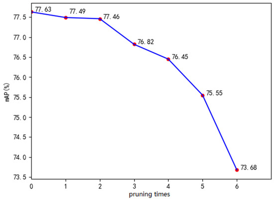
Figure 7. The mAP with 6 prunings.

Table 4. The mAP, model size and elapsed time with 6 prunings.

Pruning Times	mAP (%)	Model Size (M)	Time (ms)
0	77.63	115	50
1	77.49	80.6	43.3
2	77.46	56.9	38.5
3	76.82	40.7	35.5
4	76.45	29.7	32.8
5	75.55	21.9	30.5
6	73.68	16.4	28.0

In Table 4, the mAP loss is only 0.81% after three prunings. The model size was reduced from 115 M to 40.7 M. The elapsed time for a single image was reduced from 50 ms to 35.5 ms. Compared with the original SSD network, the mAP increased by 2.52%, while the elapsed time was reduced by 0.7 ms.

In order to test the scalability of the model, we tested 4952 images on the PASCAL VOC test set. The test results, with a confidence threshold of 0.3, are shown in Table 5.

Table 5. Experiment results of the PASCAL VOC test set.

Class	Numbers	Correct Detection	False Detection	Missed Detection	Overall Accuracy
Aero	311	311	0	0	100%
Bike	389	375	1	13	96.4%
Bird	576	554	4	18	96.18%
Boat	393	392	0	1	99.75%
Bottle	657	640	2	15	97.41%
Bus	254	254	0	0	100%
Car	1541	1502	7	32	97.47%
Cat	370	368	0	2	99.46%
Chair	1374	1308	10	56	95.2%
Cow	329	314	4	11	95.44%
Table	299	298	0	1	99.67%
Dog	530	503	4	23	95.0%
Horse	395	387	3	5	97.97%
Mbike	369	364	1	4	98.64%
Person	5227	5174	20	33	98.98%
Plant	592	578	2	12	97.63%
Sheep	311	304	4	3	97.74%
Sofa	396	391	2	3	98.74%
Train	302	301	0	1	99.67%
Tv	361	361	0	0	100%
Total	14,976	14,679	64	233	98.01%

As can be seen from Table 5, among the 14,976 objects in 4952 images, 14,679 were detected correctly, 64 were mis-detected and 233 were missed. Among the 20 types of objects, the highest accuracy was 100%, the lowest accuracy was 95.0%, and the overall accuracy was 98.01%. This proves that the network has a good scalability.

Figure 8 shows the detection results of the original and improved SSD on the PASCAL VOC dataset. The left column is the detection result of the original SSD network. The right column is the detection result of our improved SSD network. In the first row, our method detected 2 more persons and 1 more ship than the original SSD method did. In the second row, we detected 2 more cows. In the third row, our method detected 3 more chairs. At the same time, the confidence of almost all kinds of objects were significantly improved in our method.

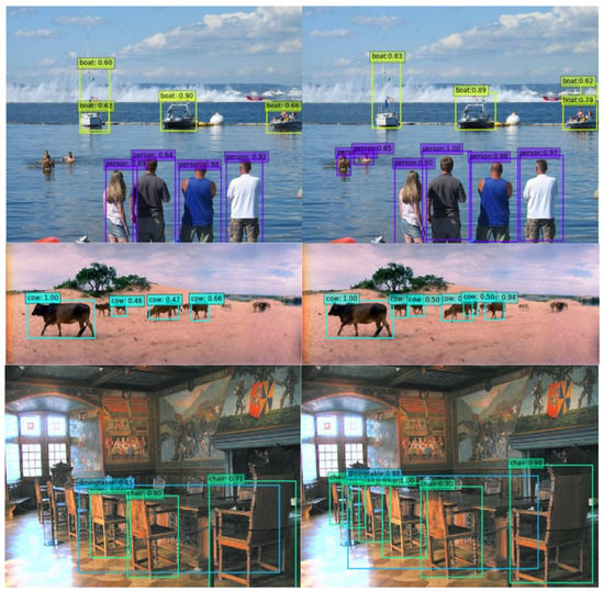
Figure 8. Detection results comparison between the original SSD and our improved SSD.

5.2. Experiment on High-Speed Railway Dataset

For the high-speed railway, any objects intruding the railway clearance will do great threat to normal operation. According to statistics, almost all intruding objects are pedestrians and normal running trains. For intrusion detection, we should detect all the intruding pedestrians and trains.

In order to test the effect of the model on the detection of high-speed railway objects intrusion, our improved SSD model obtained from the PASCAL VOC dataset was directly used for the railway intruding detection. We selected 1000 samples containing pedestrians and trains from the railway dataset. The test results are shown in Table 6.

Table 6. Experiment results on the railway dataset.

mAP (%)	Pedestrians	Trains
45.3	41.25	49.36

In Table 6, the mAP of pedestrians and trains are 41.25% and 49.36%, respectively. The model trained with the PASCAL VOC dataset is not good enough for high speed railway intruding detection. So we need to use a high-speed railway dataset that includes pedestrians and trains. We collected samples from the HangYong and BaoLan high-speed railway line at different time periods, different weather conditions, and different speed conditions. Then, we converted a series of railway traffic videos into a sequential frame of images. Because of the similar content between adjacent sequences, we sampled the image every five frames. In total, we labeled 14,760 image frames and obtained 21,053 pedestrian samples and 9231 train samples, shown in Table 7. Some of the data samples are shown in Figure 9.

Table 7. The number of each class on the railway dataset.

Class	Number
Pedestrian	21,053
Bullet Train	9231

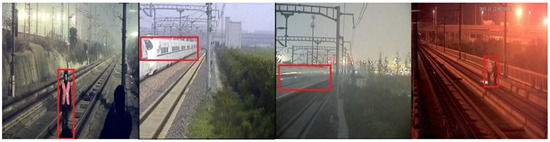
Figure 9. Samples of the railway dataset.

After the dataset setup, the improved SSD network was trained with our high-speed railway dataset. We took 80% of these samples for training and validation, and the rest for testing. The mAP, model size and elapsed time results of our method without pruning are compared with those of Faster R-CNN, YOLO, SSD and DSSD in Table 8.

Table 8. Results comparison of different methods on the railway dataset.

Method	mAP (%)	Pedestrian	Train	Model Size (M)	Time (ms)
Faster-Rcnn	75.38	70.68	80.05	512	190.2
YOLO	72.31	64.98	79.64	192	38.2
SSD	75.12	69.86	80.38	90	33.5
DSSD	79.12	77.25	80.90	569	150.8
Our Method	80.54	80.16	80.92	105	48.3

In Table 8, compared to the second best method, our method improved the precision of pedestrian detection by 2.91%. The improvement on the train detection precision is not very obvious because the train samples are all large objects. In general, our method gets the best performance in precision, the second best in model size and the third best in elapsed time.

In the above experiment, we used RGB images to train the network. In order to compare the effects of single-channel and three-channel images on the final accuracy of the network, we transformed the RGB images into brightness images for training. The training results are shown in Table 9.

Table 9. Results comparison of different methods on the brightness images.

Method	mAP (%)	Pedestrian	Train	Model Size (M)	Time (ms)
Faster-Rcnn	73.20	66.72	79.68	512	190.0
YOLO	69.5	60.96	78.04	192	38.0
SSD	73.16	66.75	79.57	90	33.4
DSSD	76.85	73.43	80.27	569	150.7
Our Method	78.21	76.01	80.41	105	48.1

From Table 9, we can see that the recognition performance of the network degrades due to the lack of chrominance information in the brightness images. But the improved SSD network still has a higher performance than other state-of-the-art networks. Compared with the RGB images, the performance of the brightness images is worse. Consequently, we use the RGB images for the recognition.

In order to reduce the model size and elapsed time, the improved SSD is pruned with the same L1 norm criterion. The pruning results are shown in Table 10.

Table 10. Pruning results of the railway dataset.

Pruning Times	mAP (%)	Pedestrian	Train	Model Size (M)	Time (ms)
0	80.54	80.16	80.92	105	48.3
1	80.20	79.79	80.62	71.8	41.4
2	80.17	79.72	80.63	49.5	36.8
3	80.09	79.59	80.59	34.4	33.2
4	79.88	79.35	80.42	24.4	31.0
5	79.28	78.5	80.05	17.4	29.8
6	78.41	77.05	79.78	12.6	27.1

In Table 10, the mAP loss is 0.66%, 1.26% and 2.13% after 4, 5 and 6 prunings. It should be noted that after 4, 5 and 6 prunings, the average precision of pedestrians decreased by 0.81%, 1.66% and 3.11%, respectively, and the average precision of trains decreased by 0.5%, 0.87% and 1.14%, respectively. The main reason for this is that the pedestrian objects are smaller than those of trains. With the same criterion as the PASCAL VOC dataset, the precision loss threshold is 1%. Consequently, we pruned the improved SSD network 4 times. After the 4th pruning, the model size was reduced from 105 M to 24.4 M. The elapsed time for a single image was reduced from 48.3 ms to 31.0 ms. Compared with the original SSD network, the mAP increased by 4.74%, while the elapsed time was reduced by 2.5 ms. Figure 10 shows the pedestrian detection results of the original SSD (Figure 10a) and our improved SSD (Figure 10b) in the high-speed railway dataset.

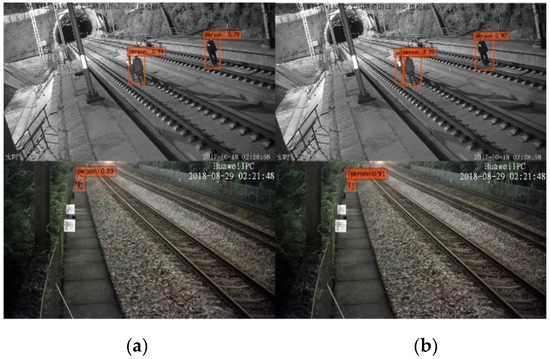
Figure 10. Comparison between the original SSD and our improved SSD. (a) Recognition effect of the SSD. (b) Recognition effect of the improved SSD.

In the first row of Figure 10, the original SSD detects the left two pedestrians as one. However, our method detects all three pedestrians. In the second row, our method detects one more person than the original SSD does. At the same time, the confidence of all objects is improved significantly in our method.

Finally, we tested with 2952 images from the test set. There are 1386 bullet trains and 3484 pedestrians (there may be multiple pedestrians in one image). We set the confidence threshold to 0.4 to test the images in the test set. The test results are shown in Table 11.

Table 11. Experimental results on the railway test set.

Class	Actual Number	Predicted as Pedestrian	Predicted as Train	Missed
Pedestrian	3484	3462	0	22
Bullet train	1386	0	1386	0

As can be seen from Table 10, among the 3484 pedestrians, 3642 can be detected. 22 are missed, and the number of false detections is 0. Among the 1386 trains, all of them can be detected, and both mistakes and missed detections are 0. The detection accuracy can reach 99.55%, the mistake rate is 0, and the miss rate is 0.45%, which can effectively perform the railway clearance intrusion detection.

In order to compare the influence of light intensity on the detection results, we divided the test set into two parts of 1723 strong light images and 1229 non-strong light images. Some of the data samples are shown in Figure 11a,b. The detection results are shown in Table 12.

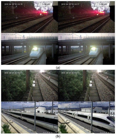
Figure 11. Images with different light intensities. (a) strong-light images. (b) non -strong light images.

Table 12. Experimental results on the strong light and non-strong light.

Light	Class	Actual Number	Predicted as Pedestrian	Predicted as Train	Missed
Strong	Pedestrian	2178	2160	0	18
	Bullet train	706	0	706	0
Non-strong	Pedestrian	1306	1302	0	4
	Bullet train	680	0	680	0

In Table 12, there are more missed detections for strong light images than for non-strong light images because of the strong light interference with the same confidence threshold as Table 11. All pedestrians and trains can be detected when we set the confidence threshold to 0.35. Consequently, the detection performance can also be improved by adjusting the reasonable threshold.

6. Conclusions

In this paper, we proposed a novel SSD network structure by deconvolving the high-level features to a low level and fusing them with original low-level features to improve their semantic information. The mAP of the improved SSD network is higher than for the other three state-of-art methods. We proposed the L1 norm criterion of the convolution kernel to prune the SSD network to decrease the calculation load. We also used a high-speed railway dataset containing ground truth information of intruding pedestrians and bullet trains. Our algorithm performs best on both the PASCAL VOC and railway datasets.

In the future, we plan to use a larger high-speed railway dataset with more types of intrusion objects, and we will conduct further research and compression methods to obtain a better detection performance.

References

- Brutzer, S.; Höferlin, B.; Heidemann, G. Evaluation of background subtraction techniques for video surveillance. In Proceedings of the 2011 IEEE Conference on Computer Vision and Pattern Recognition (CVPR 2011), Colorado Springs, CO, USA, 20–25 June 2011; pp. 1937–1944. [Google Scholar]
- Wang, Y.; Yu, Z.; Zhu, l. Fast feature extraction algorithm for high-speed railway clearance intruding objects based on CNN. Chin. J. Sci. Instrum. 2017, 38, 1267–1275. [Google Scholar]
- LeCun, Y.; Bottou, L.; Bengio, Y.; Haffner, P. Gradient-based learning applied to document recognition. Proc. IEEE 1998, 86, 2278–2324. [Google Scholar] [CrossRef]
- Krizhevsky, A.; Sutskever, I.; Hinton, G.E. Imagenet classification with deep convolutional neural networks. In Proceedings of the 26th Advances in Neural Information Processing Systems (NIPS 2012), Lake Tahoe, Nevada, USA, 3–6 December 2012; pp. 1097–1105. [Google Scholar]
- Simonyan, K.; Zisserman, A. Very deep convolutional networks for large-scale image recognition. arXiv 2014, arXiv:1409.1556. [Google Scholar]
- Szegedy, C.; Liu, W.; Jia, Y.; Sermanet, P.; Reed, S.; Anguelov, D.; Rabinovich, A. Going deeper with convolutions. In Proceedings of the 2015 IEEE Conference on Computer Vision and Pattern Recognition (CVPR 2015), Boston, MA, USA, 7–12 June 2015; pp. 1–9. [Google Scholar]
- He, K.; Zhang, X.; Ren, S.; Sun, J. Deep residual learning for image recognition. In Proceedings of the 2016 IEEE Conference on Computer Vision and Pattern Recognition (CVPR 2016), Las Vegas, NV, USA, 26–30 June 2016; pp. 770–778. [Google Scholar]
- Girshick, R.; Donahue, J.; Darrell, T.; Malik, J. Rich feature hierarchies for accurate object detection and semantic segmentation. In Proceedings of the 2014 IEEE Conference on Computer Vision and Pattern Recognition (CVPR 2014), Columbus, OH, USA, 23–28 June 2014; pp. 580–587. [Google Scholar]
- Girshick, R. Fast R-CNN. In Proceedings of the 15th IEEE International Conference on Computer Vision (ICCV 2015), Santiago, Chile, 11–18 December 2015; pp. 1440–1448. [Google Scholar]
- Ren, S.; He, K.; Girshick, R.; Sun, J. Faster R-CNN: Towards real-time object detection with region proposal networks. In Proceedings of the 29th Advances in Neural Information Processing Systems (NIPS 2015), Montreal, QC, Canada, 7–12 December 2015; pp. 91–99. [Google Scholar]
- Redmon, J.; Divvala, S.; Girshick, R.; Farhadi, A. You only look once: Unified, real-time object detection. In Proceedings of the 2016 IEEE Conference on Computer Vision and Pattern Recognition (CVPR 2016), Las Vegas, NV, USA, 26–30 June 2016; pp. 779–788. [Google Scholar]
- Liu, W.; Anguelov, D.; Erhan, D.; Szegedy, C.; Reed, S.; Fu, C.Y.; Berg, A.C. SSD: Single shot multibox detector. Proceedings of 14th the European Conference on Computer Vision (ECCV 2016), Amsterdam, Netherlands, 8–16 October 2016; pp. 21–37. [Google Scholar]
- Chen, L.C.; Papandreou, G.; Schroff, F.; Adam, H. Rethinking atrous convolution for semantic image segmentation. arXiv 2017, arXiv:1706.05587. [Google Scholar]
- Li, H.; Kadav, A.; Durdanovic, I.; Samet, H.; Graf, H.P. Pruning filters for efficient convnets. arXiv 2016, arXiv:1608.08710. [Google Scholar]
- Garcia, J.J.; Ureña, J.; Hernandez, A.; Mazo, M.; Jiménez, J.A.; Alvarez, F.J.; Garcia, E. Efficient multisensory barrier for obstacle detection on railways. IEEE Trans. Intell. Transp. Syst. 2010, 11, 702–713. [Google Scholar] [CrossRef]
- Punekar, N.S.; Raut, A.A. Improving Railway safety with obstacle Detection and Tracking System Using GPS-GSM Model. Int. J. Sci. Eng. Res. 2013, 4, 288–292. [Google Scholar]
- Catalano, A.; Bruno, F.; Pisco, M.; Cutolo, A.; Cusano, A. An intrusion detection system for the protection of railway assets using fiber Bragg grating sensors. Sensors 2014, 14, 18268–18285. [Google Scholar] [CrossRef]
- Sriwardene, A.S.; Viraj, M.A.; Muthugala, J.; Buddhika, A.G.; Jayasekara, P. Vision based smart driver assisting system for locomotives. Proceedings of 8th IEEE International Conference on Information and Automation for Sustainability (ICIAfS 2016), Galle, Sri Lanka, 16–19 December 2016; pp. 1–6. [Google Scholar]
- Nakasone, R.; Nagamine, N.; Ukai, M.; Mukojima, H.; Deguchi, D.; Murase, H. Frontal Obstacle Detection Using Background Subtraction and Frame Registration. Q. Rep. RTRI 2017, 58, 298–302. [Google Scholar] [CrossRef]
- Pu, Y.R.; Chen, L.W.; Lee, S.H. Study of moving obstacle detection at railway crossing by machine vision. Y.-R. Pu. Inf. Technol. J. 2014, 13, 2611–2618. [Google Scholar] [CrossRef]
- Guo, B.; Zhou, X.; Lin, Y.; Zhu, L.; Yu, Z. Novel Registration and Fusion Algorithm for Multimodal Railway Images with Different Field of Views. J. Adv. Trans. 2018, 10, 1–16. [Google Scholar] [CrossRef]
- Tastimur, C.; Karakose, M.; Akin, E. Image Processing Based Level Crossing Detection and Foreign Objects Recognition Approach in Railways. Int. J. Math. Electron. Comput. 2017, 1, 19–23. [Google Scholar] [CrossRef]
- Viola, P.; Jones, M. Rapid object detection using a boosted cascade of simple features. In Proceedings of the 2001 IEEE Conference on Computer Vision and Pattern Recognition (CVPR 2001), Kauai, HI, USA, 8–14 December 2001; pp. 511–518. [Google Scholar]
- Dalal, N.; Triggs, B. Histograms of oriented gradients for human detection. In Proceedings of the 2005 IEEE Conference on Computer Vision and Pattern Recognition (CVPR 2005), San Diego, CA, USA, 20–26 June 2005; pp. 886–893. [Google Scholar]
- Chen, B.H.; Shi, L.F.; Ke, X. A Robust Moving Object Detection in Multi-Scenario Big Data for Video Surveillance. IEEE Trans. Circuits Syst. Video Technol. 2018, 5, 1–14. [Google Scholar] [CrossRef]
- Messay-Kebede, T.; Narayanan, B.N.; Djaneye-Boundjou, O. Combination of Traditional and Deep Learning based Architectures to Overcome Class Imbalance and its Application to Malware Classification. In Proceedings of the NAECON 2018-IEEE National Aerospace and Electronics Conference. (NAECON2018), Dayton, OH, USA, 23–26 July 2018; pp. 73–77. [Google Scholar]
- Felzenszwalb, P.F.; Huttenlocher, D.P. Efficient graph-based image segmentation. Int. J. Comput. Vis. 2004, 59, 167–187. [Google Scholar] [CrossRef]
- Uijlings, J.R.; Van De Sande, K.E.; Gevers, T.; Smeulders, A.W. Selective search for object recognition. Int. J. Comput. Vis. 2013, 104, 154–171. [Google Scholar] [CrossRef]
- He, K.; Zhang, X.; Ren, S.; Sun, J. Spatial pyramid pooling in deep convolutional networks for visual recognition. IEEE Trans. Pattern Anal. Mach. Intell. 2015, 37, 1904–1916. [Google Scholar] [CrossRef] [PubMed]
- Sermanet, P.; Eigen, D.; Zhang, X.; Mathieu, M.; Fergus, R.; LeCun, Y. Overfeat: Integrated recognition, localization and detection using convolutional networks. arXiv 2013, arXiv:1312.6229. [Google Scholar]
- Lin, T.Y.; Goyal, P.; Girshick, R.; He, K.; Dollár, P. Focal loss for dense object detection. In Proceedings of the 16th IEEE International Conference on Computer Vision (ICCV 2017), Venice, Italy, 22–29 October 2017; pp. 2980–2988. [Google Scholar]
- Fu, C.Y.; Liu, W.; Ranga, A.; Tyagi, A.; Berg, A.C. DSSD: Deconvolutional single shot detector. arXiv 2017, arXiv:1701.06659. [Google Scholar]
- Amato, G.; Carrara, F.; Falchi, F.; Gennaro, C.; Vairo, C. Car parking occupancy detection using smart camera networks and deep learning. In Proceedings of the 2016 IEEE Symposium on Computers and Communication (ISCC), Messina, Italy, 27–30 June 2016; pp. 1212–1217. [Google Scholar]
- Wang, J.; Zheng, H.; Huang, Y.; Ding, X. Vehicle type recognition in surveillance images from labeled web-nature data using deep transfer learning. IEEE Trans. Intell. Transp. Syst. 2017, 99, 1–10. [Google Scholar] [CrossRef]
- Hu, C.; Bai, X.; Qi, L.; Chen, P.; Xue, G.; Mei, L. Vehicle color recognition with spatial pyramid deep learning. IEEE Trans. Intell. Transp. Syst. 2015, 16, 2925–2934. [Google Scholar] [CrossRef]
- Ye, T.; Wang, B.; Song, P.; Li, J. Automatic railway traffic object detection system using feature fusion refine neural network under shunting mode. Sensors 2018, 18, 1916. [Google Scholar] [CrossRef] [PubMed]
- Howard, G.; Zhu, M.; Chen, B.; Kalenichenko, D.; Wang, W.; Weyand, T.; Adam, H. Mobilenets: Efficient convolutional neural networks for mobile vision applications. arXiv 2017, arXiv:1704.04861. [Google Scholar]
- Iandola, F.N.; Han, S.; Moskewicz, M.W.; Ashraf, K.; Dally, W.J.; Keutzer, K. SqueezeNet: AlexNet-level accuracy with 50x fewer parameters and<0.5 MB model size. arXiv 2016, arXiv:1602.07360. [Google Scholar]
- Courbariaux, M.; Bengio, Y.; David, J.P. Binaryconnect: Training deep neural networks with binary weights during propagations. In Proceedings of the 29th Advances in Neural Information Processing Systems (NIPS 2015), Montreal, QC, Canada, 7–12 December 2015; pp. 3123–3131. [Google Scholar]
- Han, S.; Mao, H.; Dally, W.J. Deep compression: Compressing deep neural networks with pruning, trained quantization and huffman coding. arXiv 2015, arXiv:1510.00149. [Google Scholar]
© 2019 by the authors. Licensee MDPI, Basel, Switzerland. This article is an open access article distributed under the terms and conditions of the Creative Commons Attribution (CC BY) license (http://creativecommons.org/licenses/by/4.0/).