Assessment of Deep Learning Methodology for Self-Organizing 5G Networks

Abstract

In this paper, we present an auto-encoder-based machine learning framework for self organizing networks (SON). Traditional machine learning approaches, for example, K Nearest Neighbor, lack the ability to be precisely predictive. Therefore, they can not be extended for sequential data in the true sense because they require a batch of data to be trained on. In this work, we explore artificial neural network-based approaches like the autoencoders (AE) and propose a framework. The proposed framework provides an advantage over traditional machine learning approaches in terms of accuracy and the capability to be extended with other methods. The paper provides an assessment of the application of autoencoders (AE) for cell outage detection. First, we briefly introduce deep learning (DL) and also shed light on why it is a promising technique to make self organizing networks intelligent, cognitive, and intuitive so that they behave as fully self-configured, self-optimized, and self-healed cellular networks. The concept of SON is then explained with applications of intrusion detection and mobility load balancing. Our empirical study presents a framework for cell outage detection based on an autoencoder using simulated data obtained from a SON simulator. Finally, we provide a comparative analysis of the proposed framework with the existing frameworks.

1. Introduction

The basis of 5G evolution has five pillars: disruptive technologies [1], device centric architecture, millimeter wave (MM wave), Massive Multiple Input Multiple Output (MIMO), smarter devices for device-to-device (D2D) communication, and native support for machine-to-machine (M2M) communication for low-data rate services, low rate devices, and low latency data transfer.

For a digital environment with a highly interactive machine ecosystem, the future cellular network system has to be a neural bearer to interact with the changing environments and the provision of the sophisticated requirements of the complicated services. Artificial intelligence (AI) is the 5G technology that is capable of enhancing the interactive and decision making capabilities of the network and equipping the network to mine, train, sense, reason, act, and predict. An AI-powered 5G cellular network can be envisioned as a user-centric spectrum efficient (SE) and energy efficient (EE) nervous system of a digital society. Automated mobile networks with minimized human intervention in cellular network management are termed self-organizing networks (SONs). Self organizing networks are key ingredients for improving and optimizing operations, administration, and maintenance (OAM) activities within the cellular network. SONs utilize their self-configuration, self-optimization, and self-healing abilities to reduce the costs of installation and network management of wireless networks. Many state-of-the-art SON solutions are available on the market including AirHop’s eSON from Jio and AirHop communications [2], which received the 2016 Small Cell Forum Heterogeneous Network Management Software and Service reward [3]. However, the SON solutions available in the market are based on the following:

• Automated information processing limited to low complexity solutions like triggering and heuristics;
• Many operations are done manually; large network data is not utilized;
• Coordination of SON functions is not done yet;
• Self optimization is not extended beyond the Radio Access Networks (RANs) segment.

Therefore, it is a requirement of a cognitive and an intuitive network management not only to configure, manage, and optimize the network but also to teach the network data to behave and interact with the changing situations and requirements within the network in the future. In this paper, the use of the deep learning method is assessed for application in 5G self organizing networks (SON). Many processes involved in the management and operation of cellular networks require automation to reduce or avoid human involvement, which is often time consuming and tedious. Cell outage detection, intrusion detection, and mobility load balancing are strenuous tasks to manage and configure properly. A recent network outage incident in the UK cost Ericsson 100 million pounds in damage [4]. The use of an AI-powered intelligent SON could have saved Ericsson these costs. A few decades ago, machine learning (ML) was a less important field, but with the progress of computation power and graphical processing units (GPUs) and the increasing availability of valuable data availability, the field of ML has advanced by leaps and bounds. All of these factors have driven modern research to unleash the value of the data by applying state-of-the-art ML techniques. Common machine learning techniques including supervised or unsupervised methods work traditionally, and their results are hindered by various pitfalls including manual feature extraction, slow processing, and computation. Therefore, deep learning has emerged as an alternate ML technique to solve notoriously hard natural language processing, computer vision, and object detection and recognition problems. Deep learning aims to produce machines with full capability to interact with the environment, even if unexpected and strange scenarios arise. Therefore, by applying AI to future cellular networks, it will be possible to vanquish numerous notoriously hard tasks in wireless networks and systems. This paper first introduces deep learning and its applications in different fields, including wireless telecommunication. Then, SONs and finally deep learning for SONs are presented. The paper proposes a deep learning based framework using autoencoders (AE) for three SON cases: firstly, cell outage detection, secondly mobility load balancing, and thirdly, intrusion detection. Each case is discussed separately. The main contributions of the paper are as follows:

• We propose an autoencoder-based framework for cell outage detection;
• Our empirical study validates the proposed framework;
• Finally, the paper presents a comparative analysis of the proposed framework with the traditional frameworks.

2. Related Research Work

IBM is flourishing with AI-based WATSON, Apple has showcased Siri on the market, Google has brought out Google Now, Amazon has Alexa, Facebook has virtual assistants or Chat bot, and Microsoft has hit the market with Cortana. A significant amount of research in the wireless network communication field is also focusing on the application of advanced machine learning techniques (deep learning) to embrace the intelligence and cognition within the system in an autonomous manner. A survey of the literature involving ML algorithms applied to self-organizing cellular networks is presented in [5]. This shows the great interest of researchers in applying artificial intelligence to wireless networks. An automatic and self-organized Reinforcement Learning (RL)-based approach for Cell Outage Compensation (COC) is presented in [6]. Similarly deep Q-learning has been used in network optimization [7]. The use of deep Q-learning for self-organizing network fault management and radio performance improvement is presented in [8]. The deep convolutional neural network is applied for intelligent traffic control for wireless network routing in [9]. Multiple layer perceptron (MLP) is applied for transmitting power control in device-to-device communications in [10]. A data-driven analytic framework for automating the sleeping cell detection process in an long term evolution (LTE) network using minimized drive testing functionality, as specified by 3GPP in Release 10, is discussed in [11]. To the best of our knowledge, deep learning methods have not yet been applied to cell outage detection, mobility load balancing, or intrusion detection. Our work is the first to apply the deep learning method, namely the use of autoencoders, to solve the above-mentioned networking problems to achieve an intelligent cognitive system for 5G self organizing networks.

3. From Machine Learning to Deep Learning

Machine learning consists of computer programs that learn from data instead of pre-programmed instructions. Machine learning tasks are commonly categorized into three different types: supervised learning, unsupervised learning, and reinforcement learning. More recently, there has been an increasing interest in combining supervised and unsupervised approaches to form semi-supervised learning. In supervised learning, the task is to learn the mapping from input $\mathbf{x}$ to output y, given a dataset of $(\mathbf{x},y)$ pairs. A typical problem in supervised learning is classification. In classification, every sample $\mathbf{x}$ in the dataset belongs to one of M classes. The class of each sample is given by a label that has a discrete value $\{0,\dots ,M-1\}$. When the labels in the above example are real values (continuous), this task is known as regression problem. In unsupervised learning, the dataset only consists of samples and does not have labels. Typically, the aim of unsupervised learning is to find patterns that have some form of regularity. Usually, some model is fit to the data with the goal of modeling the input distribution. This is known as density estimation in statistics. Unsupervised learning can also be used for extracting features for supervised learning. In semi-supervised learning, the number of labeled samples is too small, while there is usually a large number of unlabeled samples. This is also a typical case in real-world situations. The goal of semi-supervised learning is to find a mapping from $\mathbf{x}$ to y but also to somehow make the unlabeled information useful for the mapping task. At least, the performance of the semi-supervised model needs to improve compared to the supervised model.

Recently, the field of deep learning or deep neural networks has received a lot of attention from the machine learning community due to its success and performance in many machine learning tasks. Deep learning has surpassed the traditional machine learning techniques because of its greater computation power, automatic feature extraction, and the development of GPUs. Deep learning addresses a famous problem in machine learning called the problem of representation.The motivation behind deep learning is to model how the human brain works. As an example, let us consider the problem of recognizing a face using data in the form of images. We know that some of the important features in a human face are the nose, eyes, and mouth. However, looking at just one single pixel or even a set of pixels of the image tells very little about the image. However, on the other hand, if we transform the data many times, we might be able to tell what the image is, because of the high number of representations we get in the form of important features. Deep learning has been able to achieve major breakthroughs in speech recognition, object recognition, image segmentation, and machine translation [12]. The scientific contributions and developments in the deep learning method and the structure of the models have provided the ground work for the advances in such a large variety of applications [12].Therefore, it may be possible for cellular networks to obtain the benefits of deep learning research, especially in the era of 5G [13,14].

3.1. What Is Deep Learning?

Deep learning is based on almost the same concepts as machine learning; however, all the recent success in deep learning is mainly based on the artificial neural networks (ANN). Research on artificial neural networks can be traced back to as early as the 1940s [12]. For many years, ANNs were less popular, and that is why the current popularity appears new. Roughly, there have been three eras of research in deep learning: the early 1940s–1960s, when the field was known as cybernetics; the 1980s–1990s, when it was called connection-ism; and the current surge started in 2006, which is called deep learning. Early development on deep learning algorithms was inspired by computational models of how the brain works or learns. This is the reason why, for a long time, research in deep learning went by the name of artificial neural networks (ANN).

The first neuron model was presented in [15]. Later, the first perceptron learning algorithm was presented in [16]. Since then, many varied models and learning algorithms have been introduced such as the Hopfield networks [17], self-organizing maps [18], Boltzmann machines [19], multi-layer perceptrons [20], radial-basis function networks [21], autoencoders [22], and sigmoid belief networks [23].

Deep learning solves the problem of representation learning by enabling computers to build complex concepts out of simpler concepts. Figure 1 (www.iro.umontreal.ca/bengioy/talks/icml2012-YB-tutorial.pdf) shows an example of representation learning, as discussed in the introduction section.

The goal of modern deep learning is to make algorithms that are successful in solving tasks that are easy for humans. Humans are good at tasks such as recognizing objects and understanding language [12]. Previously, many machine learning methods solved such tasks by hand-crafted features and by providing prior knowledge to the system. On the other hand, deep learning motivates the learning of features from the data so that the model learns to do what is expected from it. This is more like how humans learn at a young age. In this kind of machine learning approach, the system improves its performance through increased experience or more training. Therefore, deep learning is essentially machine learning that is tailored for deep models.

The recent progress in deep learning has been exclusively based on deep neural network models. The concept of depth or the determination of whether a model is deep is based on the fact that the structure of the model should consist of multiple layers that represent the level of abstraction, and each layer should adapt to model training. The features in the lower levels (layer) of the model (neural network) should progressively combine to form higher level (layer) features [12]. There are three types of DL techniques:

Supervised Learning: In supervised learning, the network is fed example inputs with labels and their desired labeled outputs. The main target of this method is to get a result that can better generalize the unseen data according to the training process and map inputs to outputs well. Supervised learning has been widely applied to solve channel estimation issues in cellular networks. Multiple layer perceptron (MLP), convolutional neural network (CNN), and recurrent neural networks can be used as supervised learning techniques.

Unsupervised Learning: In unsupervised learning, unlabeled input data is fed to the network; therefore, the network has to learn the hidden patterns in the input data on its own to produce a generalized output. In unsupervised learning, the model or network aims to find patterns or representations in the input data. In deep learning, the restricted Boltzmann machines (RBMs), autoencoders (AE), and generative adversarial networks (GAN) are unsupervised techniques while CNN, RNN, and MLP can also be unsupervised.

Reinforcement Learning: In reinforcement learning, the agent reaches the target goal by interacting with its environment. Although the agent does not have exact knowledge of the output goal, the agent takes actions to maximize the reward to achieve the target goal. The pattern recognition ability enhances learning in reinforcement learning. Deep reinforcement learning (DRL) is the reinforcement learning technique of DL, while MLP, CNN, and RNN can also be reinforcement learning types.

3.2. Training Deep Neural Networks

The training of deep neural networks is quite similar to any other machine learning model. The central method is gradient descent, which minimizes a cost function. The cost functions used in deep learning are also more or less the same as the ones used for other parametric models such as the linear models [12]. The difference is that the cost functions in neural networks cannot be optimized using convex optimization methods due to the non-linearity implemented in the neural network model. In practice, the stochastic gradient descent method is used for deep learning.

After the initial setup, there are some important factors to consider when training a deep learning model. It is always better to use more data if it is available as compared to training different models. The performance of the model has to be measured from the test data; if the performance on the test data is good, then there is hardly anything left to do. If the training performance is good but the test performance is not good, then the first solution is to use more data. It is important to select the right hyper-parameters for the training of deep neural networks, for example, the number of hidden units in a layer, the number of hidden layers, the learning rate, and weight decay are some of the most commonly available hyper-parameters that need to be tuned. Traditionally, the tuning of hyper-parameters was considered more an art and was done by rule-of-thumb. Recently, there has been an increase in the development of methods that automatically tune all hyper-parameters [24,25,26].

The hyper-parameters build on the strong intuition of the neural network model, for example, increasing the number of hidden units increases the representational capacity of the model as well as both the time and memory cost of essentially every operation on the model. An improperly set learning rate (too high or too low) results in failed optimization, and increasing the weight decay regularizes the model so that it does not overfit the training examples. For a good understanding of training deep neural networks, we refer the reader to the book [12].

3.3. Applications of Deep Learning

Some of the successful application areas of deep learning are listed:

• Image—facial recognition, image search, machine vision
• Text—sentiment analysis, augmented search, natural language processing
• Time series—risk detection, weather prediction, economic analytics
• Sound—voice detection, speaker recognition, sentiment analysis
• Video—motion detection, real-time threat detection

The number of areas of application of deep learning is growing everyday. It is now predicted that deep learning is going to transform many industries as well as society through developments in health care, education, and business. Deep learning has been applied in fields like bioinformatics [27], medicine and health care [28], space information and weather forecasting [29], education [30], traffic and transportation [31,32], agriculture [33], robotics [34], and gaming [35].

Deep learning has been extensively applied in mobile and wireless networking [36]. State-of-the-art deep learning methods have been applied for network prediction [37], traffic classification [38], Call Detail Record (CDR) mining [39], and Quality of Experience (QoE) driven by big data analysis [40]. Deep learning techniques have produced great results in network optimization [41], routing [9], scheduling [42], resource allocation in vehicle-to-vehicle communication (V2V) [43], radio control [44], and power control [45].

From the future wireless network perspective, deep learning driven techniques will be having great impact on radio resource management (RRM), mobility management (MM), management and orchestration (MANO), service provisioning management (SPM), quality of service (QoS), and energy and spectrum efficiency for 5G and beyond.

3.4. Deep Learning Frameworks

There are many deep learning libraries and frameworks to simplify the deep learning implementation processes. Most of these libraries work with different programming languages and are built with GPU acceleration. The most commonly used deep learning frameworks are

TensorFlow: TensorFlow, developed by Google, is the most common deep learning library [46]. It supports python, C, Java, and GO programming languages. Many high level programming interfaces, like Keras, Luminoth, and TensorLayer, are built on TensorFlow. TensorFlow enables computation graphs on CPUs, GPUs, and even on mobile devices.

Caffe(2): Berkeley AI Research has developed a dedicated deep learning framework named Caffe2 [47]. Caffe2 has become a very flexible framework that enables users to build highly efficient models. Caffe(2) allows neural networks to be trained on multiple GPUs within distributed systems and supports deep learning implementations on mobile operating systems, such as iOS and Android.

(Py)Torch: Originally, (Py)Torch was developed in Lua language, but later an improved Python version was released. (Py)Torch [48] is a lightweight toolbox that can run on embedded systems, such as smartphones, but lacks comprehensive documentations.

Theano: Theano [49] is a Python library that provides both GPU and CPU modes. It allows the efficient optimization and evaluation of computations involving multi-dimensional data. It provides both GPU and CPU modes.

MXNET: MXNET [50] is a flexible deep learning library that provides interfaces for multiple languages (e.g., C++, Python, Matlab, R, etc.). MXNET provides fast numerical computation for both single machine and distributed ecosystems. It wraps work flows that are commonly used in deep learning into high-level functions, such that standard neural networks can be easily constructed without substantial coding effort.

Chainer: Chainer [51] is a Python-based, flexible deep learning framework. It provides dynamic computational graphs, as well as object-oriented high-level APIs to build and train neural networks. It supports CUDA and cuDNN using CuPy for high performance training and inference.

Microsoft Cognitive Toolkit/CNTK: Microsoft Cognitive Toolkit/CNTK [52] is known for the easy and flexible training of deep learning models. CNTK is an open source library, and it is supported by different interfaces such as Python, C++, and the command line interface.

Keras: Keras [53] is an easy-to-use, simple deep learning library for building deep learning models by stacking multiple layers. Keras is part of TensorFlow’s core API group. Keras is written in Python and is capable of running on top of TensorFlow, CNTK, or Theano. It runs seamlessly on CPUs and GPUs.

4. Enabling 5G with SON and Deep Learning

There has already been a lot of work done on the use of machine learning approaches in the cellular network domain [54,55,56,57,58,59]. In this section, we describe how SON and deep learning could play an important roles in jointly driving future cellular networks [60]. When the 1G mobile networks were deployed, they made the connection between people instead of places, as was done in predecessor technology, possible. Similarly, when deployed, 5G mobile networks will make the connection between anything possible, instead of just people [61]. Three key areas have been identified where major changes will occur with 5G. The networks will utilize mmWave, massive MIMO, and densification [62]. 5G networks are more about D2D communication, which means there will be a higher number of users and more demand for capacity. An effective way to increase capacity is by making the cells smaller, which has also been a trend in the past. This leads to densification, and it is projected that to enable the kind of capacity required, there will need to be a 40–50-fold increase in densification [61]. This number far exceeds other sources of change in the mmWave and massive MIMO that will be deployed in 5G. Therefore, SON and deep learning will have the highest potential impacts on 5G.

The dynamic and unpredictable factors involved in 5G networks, for example, spikes in social media usage, can occur at any time, demand fast and efficient automation. The task of SON and deep learning is to transform data/Key Performance Indicators (KPIs) into more actionable information [63]. In general, ML consists of predictive analytics that is able to determine the probability of future events or the likelihood of any particular event occurring [63]. Although, SON automates a lot of the functions required for the management and allocation of resources, there are still problems that are solved by applying a set of rules of thumb. These rules are derived from experience and domain knowledge. SON implements a level of intelligence in the system using programmed rules and, to a lesser extent, by using ML. However, this method needs to improve due to the increase in the number of challenges faced from the dynamic and diverse traffic and network complexity.

In the current networks, monitoring relies on alarms generated at the cell level based on static thresholds. This is inefficient for 5G, which will have a dynamic nature [63]. Engineers depend on troubleshooting guides; however, there are obvious limitations to such approaches, because such guidelines implement the one-size-fits-all criteria. Such guides are only limited to, or useful for, known issues, but the future networks need to be adaptive. The time taken to resolve issues causes latency and results in customer dissatisfaction. The time taken to investigate and resolve issues increases the cost as well. The growing network technology and complexity demands automated, flexible, energy efficient, low-cost, capable, and scalable solutions [63]. In addition, the network has to be capable of continuously learning from the environment and improving its performance in mobile data delivery in terms of the user context and network context. Networks using deep learning or AI are able to provide efficient solutions to some of these problems [64,65]. Therefore, SON and deep learning could work together to resolve many of the dynamic problems in future cellular networks.

4.1. What is SON?

Self-organizing networks or simply SONs are sets of automation techniques in mobile radio access networks or cellular networks. SONs can be intelligent in the sense that they can learn from their environments while autonomously adapting to ensure reliable communication. The purpose of SONs is to automate the processes of network planning, configuration, and optimization together in order to minimize the amount of manual work required [60]. As a result, the cost of management is reduced by simplifying operational tasks through self-configuration, self-optimization, self-healing, and self-protection [13]. The key SON objectives can be simply illustrated as

• Improving the network capacity, coverage, and customer service experience by enhancing the network performance;
• Reducing the capital expenditure and operational expenditure (CAPEX/OPEX);
• Introducing autonomous and intelligent adaptability in the cellular networks through the self healing, self optimization, and self configuration properties of SON networks;
• Improving the spectral efficiency of the next-generation Radio Access Networks (RANs).

3GPP introduced the SON as a vital component of the LTE network for the first time in Release 8. Cases of SON use in SOCRATES [66] are classified according to the life cycle of different phases within the cellular network. The phases of planning, deployment, maintenance, and optimization are classified as self-configuration, self-healing, and self-optimization.

The self-configuration aspect of SON minimizes human intervention in network management. Configuration of the enhanced node based station (eNBS) is done by the self configuration algorithm. The eNB establishes a connection with the core network after detecting the core transport link. eNB performs self-testing and delivers a status report to the network management node. Self-configuration includes operational parameters, a neighbor cell list, and radio parameters.

Self-optimization optimizes the network parameters during operation based on the measurements received from the network. There are many SON functions in Release 9. The most common are

MLB: MLB manages the congestion of cells through mobility load transfer to other cells. As a result, MLB enhances the end user experience by achieving higher system capacity. MRO: MRO is an SON function that ensures complete mobility and proper handover in connected mode and cell reselection in idle mode. Inter-Cell Interference Coordination (ICIC): ICIC minimizes inter-cell interference using the same spectrum. The inter-cell interference is reduced with the coordination of physical resources from one cell to another. Random Access Channel(RACH): RACH optimization is achieved by adjusting the power control parameter or by changing the preamble format to reach the set target access delay. Coverage and Capacity Optimization (CCO): In Release 10, 3GPP defined a new SON function named coverage and capacity optimization (CCO) to achieve an optimal trade-off between capacity and coverage. Energy Saving (ES): ES, defined in Release 10, targets the end user’s quality of experience (QoE) by making the system energy efficient and environmentally friendly. Energy consumption optimization is achieved by designing network elements with low power consumption and temporarily shutting down unused capacity or nodes when not needed [67].

Self-healing stresses the maintenance of a cellular network. In cellular networks, faults are very common. Fault management is an important task in RANs. For any faulty situation, if the system cannot serve the network properly, degradation of the performance results, leaving the user with no service availability. This kind of problem results in severe revenue loss for the operator. Self-healing is therefore a key to fault management. We focus more on the three important mechanisms of self-optimization, self-healing, and self-protection. Self-optimization functions are used to analyze the performance of the network and automatically trigger the required actions. The aim of self-optimization is to maintain the quality and performance of the network without the need for human intervention or manual work. Self-healing deploys trigger and detection methods in order to protect the network from failure. The purpose of self-healing is to automatically detect and address any network operation problems. Self-protection maintains the safety and security of the network from cyber-attacks or intruders. The aim of self-protection is to detect patterns that could lead to potential threats.

5G SONs should have the capability to adjust the network if needed in certain situations, the ability to find minimum network parameter values to acquire a high optimization level, and an awareness of the current network status and any changes happening within the network. All of these built in capabilities in SON will make it more suitable and adaptable for future wireless networks.

4.2. Deep Learning-Based Anomaly Detection

One of the major causes of anomalous behavior in cellular networks is cell outage. Cell outage management is part of the self-healing process in SON. A possible solution for cell outage detection could be achieved with the deployment of an autoencoder. This could potentially lead to the development of the deep learning method for SONs given that the huge amount of data available with the realization of 5G networks. Here, we present a brief introduction of an autoencoder that is actually an artificial neural network model and explain the idea behind the possible use of autoencoders for cell outage management. The data required to implement autoencoder cell outage management could be cell level data, where the KPIs are represented, for example, by receiver response reference signal (RSRP) values and receiver response reference quality (RSRQ) values, and, in addition, the neighboring cell RSRPs and RSRQs. However, in 5G networks, due to densification, the representation KPIs could consist of a large vector of measurements which could be more suitable for deep structured autoencoders.

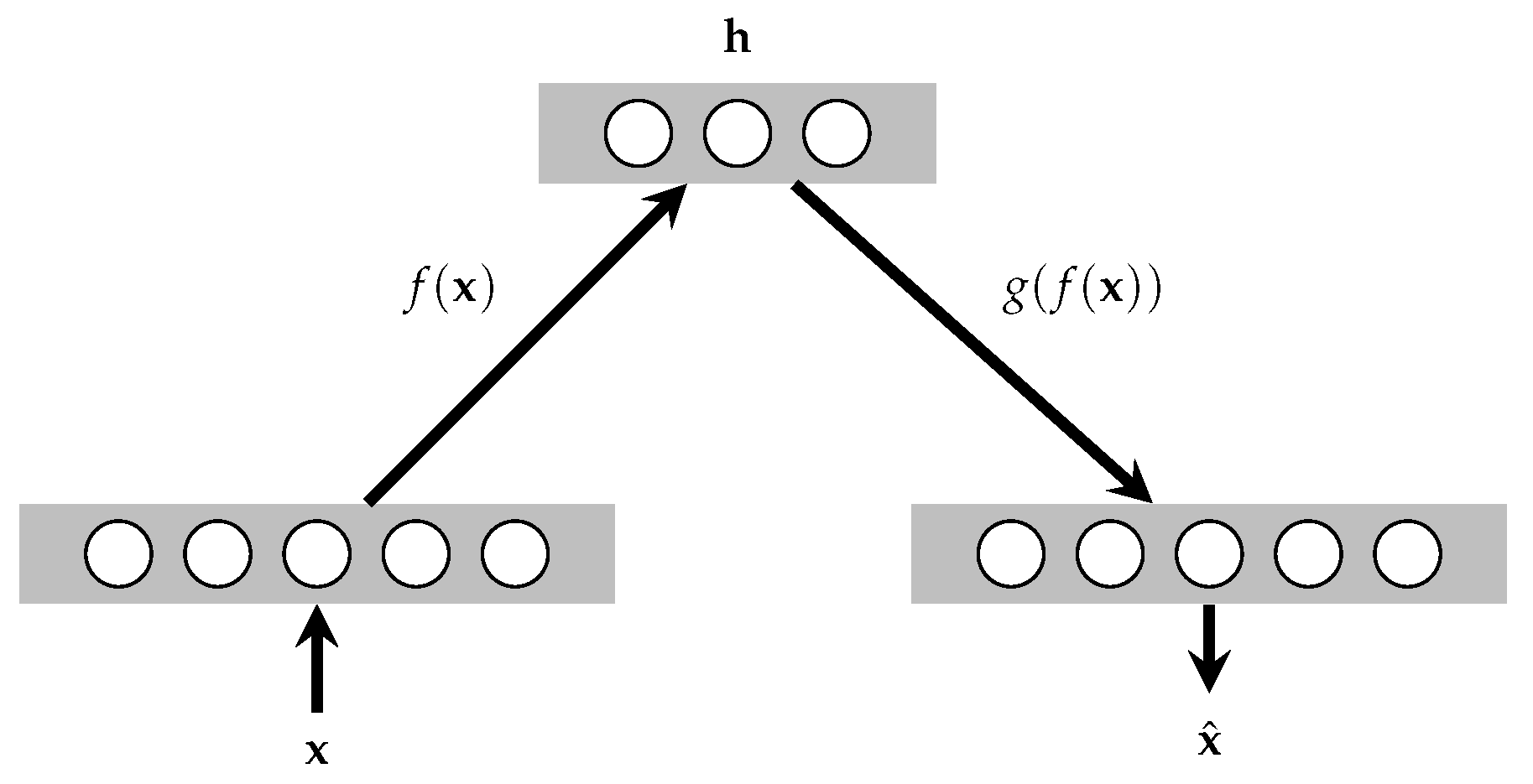
4.2.1. Autoencoders

An autoencoder is an artificial neural network that is based on the unsupervised learning approach. Autoencoders consist of two parts: the first part is called the encoder, which enables efficient coding $\mathbf{h}$ of the input data $\mathbf{x}$, and the second part is the decoder, which generates a reconstruction $\widehat{\mathbf{x}}$ of the input data. A simple depiction of the autoencoder is shown in Figure 2. The function $f(\mathbf{x})$ maps the input data to the hidden representation or code, and the function $g(f(\mathbf{x}))$ reconstructs the input data to the output representation. Typically, the encoder and decoder can be represented with the following:

• encoder: $\mathbf{h}=f(\mathbf{W}\mathbf{x}+\mathbf{b})$ and
• decoder: $\widehat{\mathbf{x}}=g({\mathbf{W}}^T\mathbf{h}+\mathbf{c}),$

where $\mathbf{b}$ and $\mathbf{c}$ are biases, and the functions $f(·)$ and $g(·)$ are non-linear mapping functions. The training consists of finding parameters $\mathsf{\Theta }=\{\mathbf{W},b,c\}$ by minimizing the following cost:

$$\begin{array}{cc}\hfill \mathcal{L}(\mathbf{x},\widehat{\mathbf{x}})=-\sum _{n=1}^N& [{\mathbf{x}}^{(n)}log({\widehat{\mathbf{x}}}^{(n)})\hfill \\ & +(1-{\mathbf{x}}^{(n)})log(1-{\widehat{\mathbf{x}}}^{(n)})],\hfill \end{array}$$

(1)

which is called the cross-entropy loss. N is the number of training samples ${\{{\mathbf{x}}^{(n)}\}}_{n=1}^N$. The cost of Equation (1) is considered when $\mathbf{x}$ and $\widehat{\mathbf{x}}\in [0,1]$. In case of linear reconstruction of $\widehat{\mathbf{x}}$, the typical choice is the squared error $\parallel \mathbf{x}-\widehat{\mathbf{x}}{\parallel }^2$.

The autoencoder can be used for cell outage detection in such a way that the model learns to reconstruct the input KPIs. It is important that the hidden layer or the coding layer is smaller than the input layer. This is because if the hidden layer is equal in size to the input layer, then the model will learn the identity function and the output of the model will be a perfect reconstruction. This is also true for case where the hidden layer is of a larger size, which can also lead to the training KPIs being over-fitted. This is also known as an over-complete case. However, it is also possible to add noise to the inputs at the input layer to avoid perfect reconstruction.

The idea is that if the autoencoder is trained on normal KPIs or data that is not anomalous, then the model will learn to reconstruct the unseen KPIs or test data that is non-anomalous with a low reconstruction error. In contrast, the use of anomalous KPIs would result in a high reconstruction error. Therefore, the use of a proper reconstruction error threshold value could help to distinguish between the anomalous and non-anomalous users.

4.2.2. Experimental Setup

A simulation study has been performed in ns-3 simulator whereby 105 mobile users were uniformly spread around 7 base stations. The base stations were spread regularly on the grid where each circle represents a base station. The users were mobile and spread uniformly across the grid. The periodic (once every 0.2 ms) MDT report generated by each of the users were recorded for about 50 s. The data has been hand labeled so that each MDT report has been assigned a label from the set {0, 1, 2, 3}. Labels 0, 1 and 2 represent normal network conditions with distinct transmit power levels. An MDT report with label 3 indicates that the corresponding user was previously being served by a BTS that has failed. Only one BTS failure is simulated. The main parameters used in the system simulation are summarized in

Table 1. Simulation parameters.

Parameter	Value
Cell Layout	Hexagonal grid
Number of cells	57 cells (19 eNodeBs, 3 sectors per eNodeB)
Number of sectors for each base station	3
Inter-site Distance	500 m
eNodeB default Tx Power	46 dBm
Number of UEs in the scenario	105
UE Distribution	Uniform
Traffic Type	Downlink Full Buffer
Simulation lengths	150 s
Cell Outage Tx Power	–50 dBm

.

In order to use the autoencoder model for cell outage detection, a machine learning framework was set up. We used L1 type regularization at the input layer and the dropout at the first hidden layer with a $50\%$ dropout rate. This helped to overcome any potential over-fitting problems. The model was trained for 100 epochs with a mini-batch size of 22 samples. The Adam training algorithm was used, and the cost function was the mean squared error. We used the Keras library in Python for the implementation of the model.

There were two phases: the detection of anomalous cases in the test KPIs and finding the nearest base stations for each test sample. After finding the nearest base-stations, it was possible to identify the base station with the most anomalous cases.

Table 2. Simulation data set parameters.

Data Set	Number of Users	Number of Cells
Data set 1	105	21
Data set 2	210	57
Data set 3	105	57
Data set 4	105	57

gives four data sets that are used to test the cell outage framework. These have been made publicly available by the authors for the readers to do their own analysis [68].

4.2.3. Dataset 1

In this section, we describe the use of one of the datasets to perform cell outage detection and base station identification given the KPIs obtained by a SON simulator. The simulation was run for 25 steps where each step was 2 s long. There were 7 base stations in total, placed at fixed locations and separated from each other with fixed distances. Each base station consisted of 3 cells, so, in total, 21 cells were simulated. There was a total of 105 users and they moved in the enclosed area with a random walk model. The data generated by the cell consisted of the measurement time, the unique ID of the user, the location co-ordinates of the user in the 2-dimensional plane, the reference signal received power, the reference signal received quality, and the label indicating whether the user was anomalous or non-anomalous. The KPI selected for the use case was reference signal received power (RSRP) and reference signal received quality (RSRQ) which are the key measures of signal level and quality for LTE networks. When a mobile user moves from one cell to other cells and performs cell selection/reselection and handover, it has to measure the signal strength and signal quality of the neighbor cells. The RSRP is the average received power of a single reference signal of resource element whereas RSRQ is the average received quality of the reference signal of resource element. RSRP measurements are used to perform user equipment (UE) Attach, cell selection, cell re-selection, handover procedures. The RSRQ measurements provide additional information when RSRP is not sufficient to make a reliable handover or cell reselection decision. Cell outage is the state of the cell when a cell is not able to serve the users due to the network performance degradation. The cell outage is caused by hardware and software failures (radio board failure, channel processing implementation error, etc.), external failures such as power supply or network connectivity failures, or even erroneous configuration. It is important to detect the cell outages as quickly as possible to recover the coverage loss and minimize the revenue loss caused by cell outages. The users effected from cell outages are termed as ’anomalous users’. The anomalous user detection is crucial step to detect the cell outages. The feature vector was $\{{\mathrm{RSRP}}^1,{\mathrm{RSRQ}}^1,{\mathrm{RSRP}}^2,{\mathrm{RSRQ}}^2,\dots ,{\mathrm{RSRP}}^9,{\mathrm{RSRQ}}^9,{\mathrm{RSRP}}^{10},{\mathrm{RSRQ}}^{10}\}$. It was clear that the units of measurement were quite different, so pre-processing was required, as described in the previous section. The simulation was manually handled from the User Interface (UI),and when a cell was broken, its transmission power from the base station was set to 0 dbm. This was not necessarily reflected in the RSRP and RSRQ values. The KPIs were preprocessed to handle missing values and then scaled between 0 and 1.

We split the KPIs into $80\%$ for training and $20\%$ for testing after the rows had been randomly shuffled. The training set only consisted of normal users, while both normal and abnormal users were part of the test set. During training, the test set was used for validation as well. Since the input vector size was 20, the first encoding layer of the autoencoder model had a size of 20, and the output layer size was the same. The autoencoder model structure was 20-12-6-6-12-20. This structure was chosen with the idea that the hidden layers would be able to compress the input information and avoid identity mapping from inputs to outputs.

4.2.4. Phase 1—Training and Testing

The machine learning framework is shown in Figure 3. The framework depicts that the model was first trained, as shown by the flow of the top graph in the left block, which is phase 1. Model training only require normal KPIs or non-anomalous data. Usually pre-processing must occur before training the autoencoder model. There could be missing values which need to be properly handled. We used the mean imputation method to address missing KPIs and then scaled the values between 0 and 1. The autoencoder was trained with the linear reconstruction cost; as a result, the parameters of the model were learned. The reconstruction cost for each sample was obtained, and this acted as the score. In the bottom graph in Figure 3, in phase 1, new unseen KPIs consisting of both anomalous and non-anomalous samples were used. Again, in this case, the KPIs were preprocessed in a similar way to the training KPIs. The trained model was then used to reconstruct the test samples, and as a result, the reconstruction error for each input sample of the test KPIs was obtained. Then, a decision function was formed based on the fact that small reconstruction values represent non-anomalous samples and high reconstruction values represent anomalous samples.

4.2.5. Phase 2—Finding the Nearest Base Station for Each Anomalous User

After the detection of the anomalous users in the given test KPIs, phase 2 was implemented, as shown in the right block in Figure 3. The second phase consisted of finding the nearest base station for each anomalous user by using the Euclidean distance. Another approach used for identification is cell outage, which is based on z-score computation, as described in [69]. A similar approach can be implemented in the proposed framework, as shown in the Figure 3. Finally, the base station with the highest number of anomalies can be identified as the broken base station, or the z-score computed for the test set anomalies can be compared to the training set or reference z-score values for the identification of broken stations.

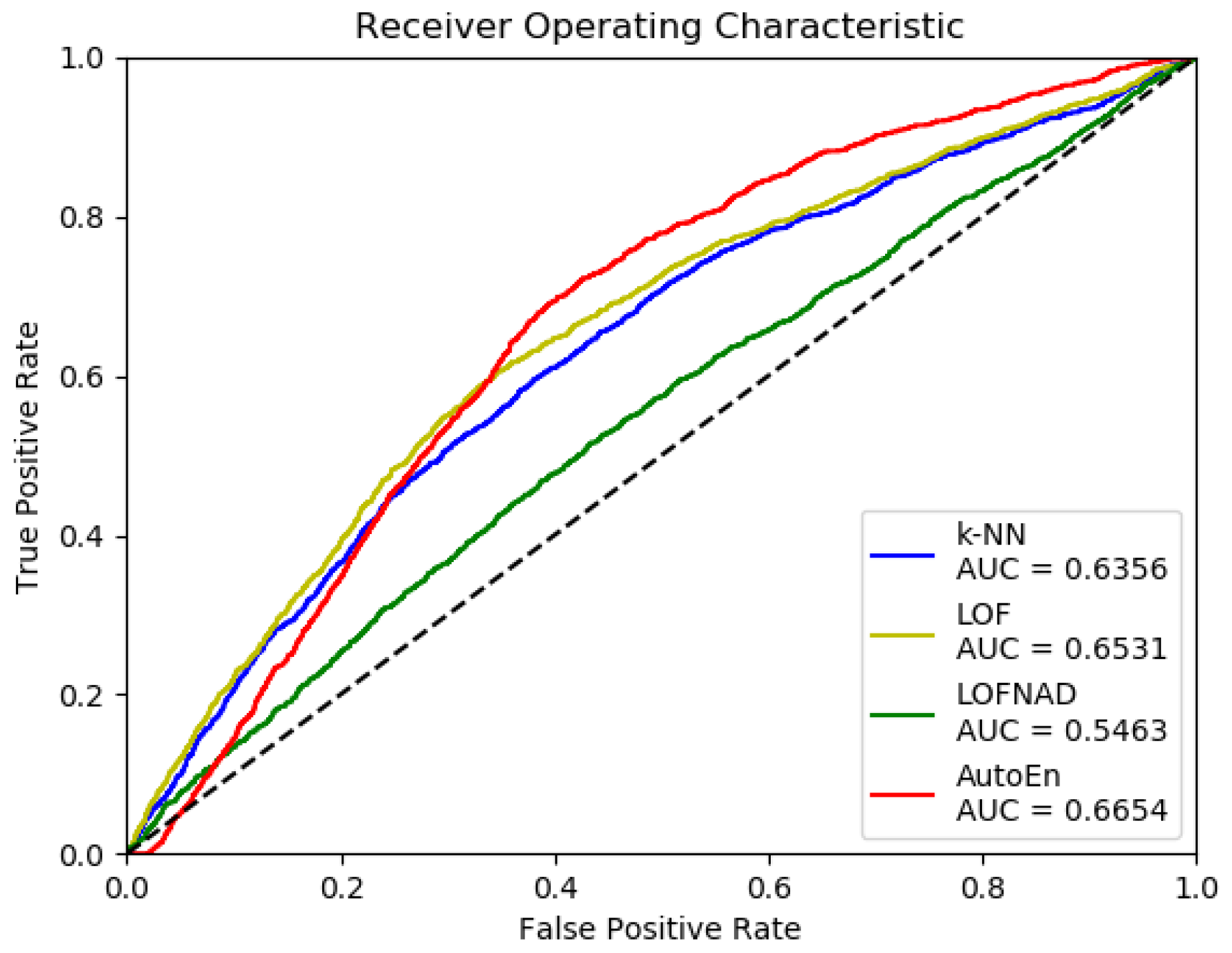
The result from the autoencoder is represented in Figure 4, which shows the ROC curves for the test set predictions. We can also observe the confusion matrix for the results. In this case, we have the number of true positives, the number of true negatives, the number of false positives, and the number of false negatives. In the next step, we identified the outage cells and their nearest base stations. This was then used to find the broken base-station. The maximum number of anomalies in this case was associated to the fifth base station. The reference z-score was also used to find the broken base station.

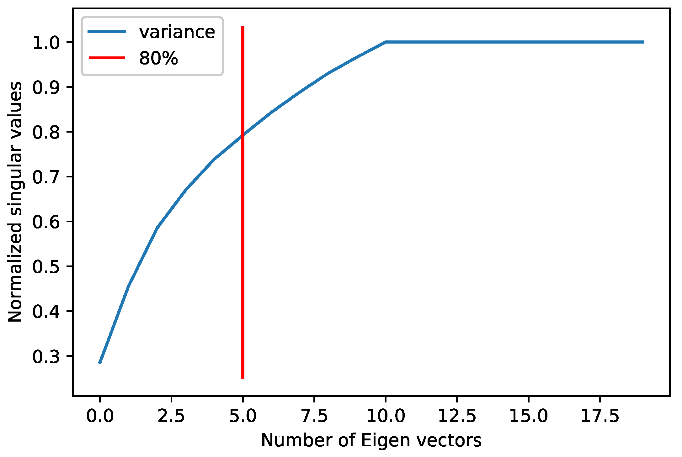
The results of the autoencoder were compared with those from nearest-neighbor approaches such as the k-nearest neighbor (k-NN), the local outlier factor (LOF) analysis, and the LOF with the average density, as shown in the Figure 4. The nearest neighbor approaches require the dimensionality of the input data to be reduced, because distance-based approaches are not suitable for high dimensional data. In this case, we used the principal component analysis (PCA) to reduce the dimensionality of the data, and we observed that $80\%$ of the variance in the data was captured by five PCA components. Therefore, when training the nearest neighbor approaches, we used the five-dimensional PCA reduced data. Figure 5 shows the normalized singular values compared to the number of PCA components.

From the results, we can observe that the autoencoder approach performs the best in terms of accuracy.

4.2.6. Dataset 2

As a second use case, we performed tests where the dataset was larger in terms of the number of users and the cell density. In this dataset, there were 57 cells and 210 users. The autoencoder setup for performing the test on this dataset was similar to that of the previous dataset. The results in terms of the ROC and AUC values are shown in Figure 6.

We compared the performance of the autoencoder with the nearest neighbor approaches in this use case as well. We observed that increasing the size of the data and density of the cells improved the performance of the autoencoder.

4.2.7. Dataset 3

As third use case, we performed a new simulation with larger network of 57 cells and 105 users. The new data set was gathered with a simulating an 80 s period of mobile network activity and produced a data set of 42,001 entries. Each entry has 114 features (in addition to data not used for detection, like location coordinates, timestamp and userID) consisting of RSRP and RSRQ values for the 57 cells. The simulation was run for 400 steps where each step was 0.2 s long. ROC-curves are presented in Figure 7.

4.2.8. Dataset 4

Finally, we performed a new simulation with same parameters: 57 cells and 105 users, again run for 400 steps where each step was 0.2 s long, simulating in total an 80 s period of mobile network activity. Each entry again had 114 features (in addition to data not used for detection, like location coordinates, timestamp and userID) consisting of RSRP and RSRQ values for the 57 cells. However labeling was done differently. We labeled as anomalous only the entries, where the cell the user was connected to went into outage, and the RSRP value for this cell dropped below –120 dB. This meant there were far fewer anomalous entries (only 22), so to balance the data set the entries were duplicated a 100 times. ROC-curves are presented in Figure 8. We also performed five-fold cross-validation for the autoencoder getting the following AUC-scores {$0.801$, $0.871$, $0.809$, $0.921$, $0.847$} with the average AUC-score of $0.850$.

4.3. Deep Learning-Based Mobility Load Balancing

A cellular network can suffer from a huge amount of traffic on a few nodes or cell congestion. In order to solve such issues, SON deploys mobility load balancing (MLB) approaches as part of the self-optimization. MLB enables load transfer between cells to improve the service quality. As challenges are posed by 5G to cellular networks, the importance of MLB becomes even greater. Moreover, 5G will consist of dense networks, meaning an increase in data, while the number of users is projected to grow as well. Previously, networks have used certain measures of different resources to determine the load of a cell, for example, the total transmitted power and total received power, interference in a cell, the handover failure rate, and the cell throughput. These kinds of variables are used usually in SON as well to analyze or determine whether the load balancing mechanisms for a cell must be activated. A drawback to these approaches is that they are generally reactive approaches, while in 5G, more proactive approaches are required so that the latency in the management is reduced. A major advantage of using machine learning, especially, artificial neural network-based approaches, is that they can predict future congestion. This kind of approach can be implemented by cellular traffic monitoring at the cell level or base station level, and then a deep neural network model can be trained to learn traffic patterns. The model would then be able to predict future traffic patterns or indicate cell congestion prior to the problem. This would allow load balancing mechanisms to be implemented early, thus resulting in a reduction in latency. A wide range of approaches has been used for load balancing; the reader is referred to a few [70,71,72].

The current load balancing mechanisms in cellular networks are based on different methods, for example, changing the coverage area of the cell depending on the load variation. Usually, the transmission power is increased or decreased to expand or reduce the cell coverage area. Other techniques include the use of antenna tilt schemes or handover parameter modification. The MLB is based on finding the optimal handover (HO) offset value between an overloaded node and a target node. This is required so that the users can be shifted to less loaded neighboring cells that are adjacent to the loaded cell. However, this is also a complex mechanism as the adjacent cells might not have enough capacity to handle additional cellular traffic. Again, in such scenarios, deep learning-based approaches could be useful due to their predictive ability.

Current state-of-the-art MLB approaches use reinforcement learning methods to dynamically adjust handover parameters. Such methods also learn with reward-based schemes. The problem is an optimization task and the parameters are adjusted according to certain predefined metrics. The load of the network is constantly monitored. If there is an increase in the load of a cell, then the network parameters can be adjusted to mitigate the problem. Deep learning based approaches can enhance the MLB methods in 5G by implementing the traffic pattern monitoring and congestion detection schemes [73,74].

4.4. Deep Learning-Based Intrusion Detection Framework

The cellular network can be a target of different attacks that lead to failure of the network services. The concept of self-protection is important for SONs in 5G. Traditionally, security requirements were for the protection of voice and text data. User identification was solved by implementing a secure SIM. The networks implemented mutual authentication between the network and users. The communication path between communicators was also made secure.

While 5G brings speed, more flexibility, new services, and easy communication, it also brings new kinds of threats. A usual threat in computer networks is the denial of service (DoS) attack. The DoS is a type of attack where a huge amount of traffic is generated on particular nodes, so much that the nodes are not able to respond to requests anymore. As 5G is going to build on the Internet of Things (IoT) concept, it will connect many devices and some will be very small. Often, the security of such small and simple devices cannot be implemented at the node level. This means that such nodes are highly vulnerable, especially to DoS attacks. Other important factors to consider are that 5G will connect many different types of networks. This means that there will be different levels of protection needed, for example, a hospital connected via the network would require special treatment as compared to a tire shop. All in all, many aspects of 5G are still under development; however, some high level decisions about security and privacy need to be agreed on between stakeholders. In the literature, many methods have been proposed for intrusion detection in cellular networks [75,76].

Machine learning methods have been successful in implementing pattern-based intrusion detection for cellular networks. Therefore, there is the potential to use machine learning and also deep learning [77] techniques in 5G. In 5G, deep learning could help in the detection and mitigation of DoS attacks via traffic monitoring and proactive prediction of unforeseen events. Other solutions could be end user equipment protection from malware, access network intrusion detection, and mobile core and IP network protection.

User equipment, such as smart-phones and tablets, is vulnerable due to the variety of connectivity options (LTE, 5G, WiFi, etc.), third-party apps, and operating systems, and the over increased data transmission. Mobile malware can get installed on user devices via apps downloaded from untrusted app stores. Malware can exploit and steal personal user data, enable DoS attacks, spam the network from a user’s device, or launch a distributed DoS attack. Attacks on the access network can be for the purpose of stealing bandwidth, tracking a specific user in a cell or multiple cells, and physical tempering of the hardware. The mobile core and IP network are also vulnerable to DoS attacks. A major drawback for ML or deep learning approaches in the detection of vulnerabilities in these networks could be the unavailability of labeled data. However, possible solutions could be semi-supervised learning approaches, where any small set of labeled data can be useful.

5. Framework Assessment for Deep Learning

The framework presented in this work consists of a graph with a single flow direction from input to output that supports the types of problems discussed in this paper. The problems of cell outage detection, intrusion detection, and mobility load balancing typically require the input to be provided as KPIs, and the method determines whether there is cell outage or intrusion happening or whether load balancing activation is required.

The current data source used to obtain the KPIs is cell level data which consists of the measurement time, the unique ID of the user, the location co-ordinates of the user in the 2-dimensional plane, the reference signal received power, and the reference signal received quality. With 5G, other sources of data will become available that will be suitable for deep learning. The data/KPI module could obtain data from different types of sources, for example, subscriber level data, such as the call drop ratio, session drop rate, and throughput, and cell level data, such as thermal noise power, channel power, channel quality indicator (CQI), and core network level and App-based data.

The pre-processing step transforms data into useful attributes. In the current framework, the KPIs are checked for missing values and proper imputation. The KPIs are also mean normalized or scaled between standard 0/1 values. This is usually what is required for a deep learning setup. The KPIs in the cell outage detection framework are also feature engineered. However, with 5G, the possibility of high dimensional data is more likely, which the current framework supports, since it does not require any low dimensional techniques, such as Principle Component Analysis (PCA) or Singular Vector Decomposition (SVD), while other frameworks usually require such methods. Autoencoder-type models or feed-forward neural networks become more powerful tools with the increase in dimensionality, especially in case of deep learning techniques.

The other nearest-neighbor-based approaches require a score to be computed, which is often a computationally expensive task. The autoencoder-based framework does not need to compute an explicit score; rather, the reconstruction error that is minimized for training the model acts as the score itself. In this way, computational time and resources are minimized by the proposed framework. The test framework also consists of a forward flow graph. The test phase of the proposed framework is fast, since it does not need to train or compute any scores. The test KPIs immediately obtain the score in terms of the reconstruction error. The threshold has to be selected manually, and the test KPIs are then classified as normal or abnormal user/cells, intrusion or non-intrusive cases, and cell loaded or cell non-loaded scenarios.

6. Comparative Analysis of Proposed Framework with the Existing Frameworks

In this section, we explain some of the advantages and/or disadvantages of adopting the proposed autoencoder-based machine learning framework. Although nearest neighbor based approaches like k-NN have been widely used and accepted as easy methods, they lack the ability to be predictive. Nearest neighbor approaches cannot be extended for sequential data in the true sense, because they require a batch of data to be trained on. Nearest neighbor approaches are suitable for high dimensional data but work well for low dimensional data. In anomaly detection, nearest neighbor approaches require the calculation of some kind of score that is usually computationally expensive. On the other hand, artificial neural network-based approaches, like the autoencoders explored for cell outage detection in this work, are able to overcome all of the above-mentioned drawbacks.

In general, ANNs have the ability to store information about the entire network, and missing information in some places does not stop the network from functioning. Once trained ANNs are able to handle missing values in the test data, the loss of performance only depends on the importance of the missing information. The structure of ANNs can be exploited in many ways, and, similarly, training the network has a large degree of freedom (DoF). ANNs learn from events and have the ability to make decisions. They also have parallel processing capability and can be run simultaneously to perform several jobs at the same time.

On the other hand, the degree of freedom in the structure and hyper-parameter space requires that such parameters are properly optimized and/or that a trial and error strategy is adopted. This results in excessive training in terms of computational time and resources. ANNs also have a strong hardware dependence, especially deep learning, where the models have large structures. Sometimes, due to unexplainable behavior, it is difficult to explain why and how the solution was attained. This is an important drawback because it reduces trust in the network. ANNs work with numerical data, and all other forms of data need to be transformed to numerical values. The

Table 3. Comparison of attributes of neural network (deep learning)-based approaches with standard nearest neighbor and other approaches.

PCA/SVD	Score Computation	Missing Data	DoF	Data Utilization	Extendable	HPC
Nearest-neighbors	✓	✓	✗	Small	Limited	✗	✗
Neural Networks	✗	✗	✓	Large	Extensive	✓	✓
Clustering	✓	✓	✗	Small	Limited	✓	✓
Support Vector	✓	✓	✓	Small	Limited	✓	✗
Probabilistic	✓	✓	✓	Small	Limited	✓	✓

shows a comparison of some of the attributes discussed with regard to standard nearest neighbor approaches and the neural network-based approaches that are used in deep learning. Table 3, compares the requirements of PCA/SVD, the requirements of explicit score computation, the reliability in the presence of missing information, the degree of freedom (DoF), the amount of data utilization, and the ability to extend and utilize high performance computation (HPC).

Due to their strength in terms of performance on very difficult problems, deep neural networks are the state-of-the-art methods. Research and development in ANNs is occurring at an extremely fast rate in the present day. The disadvantages of ANNs are quickly being reduced day-by-day, while their advantages are increasing. Deep learning and AI will be the technology of the future, and future cellular networks will require that AI is built along with them.

When compared to other frameworks, the proposed framework mainly has advantages in terms of its simplicity and the capability to to be extended with other methods. This is also the case for artificial neural network models—in general, they can be adapted to any kind of dataset. However, the major reason behind the success of current deep learning applications is the huge of amount of labeled data that the machine learning community has been able to provide. Although there has been much advancement in unsupervised and semi-supervised deep learning methods, the majority of the state-of-the-art results have been for supervised problems. So, how can we decide whether selecting the deep learning framework is suitable, for example, in the self-optimizing, self-healing and self-protection modules of SON in future networks? An important consideration for the proposed framework is its comparison in terms of computational complexity. We used the data on computational complexity of nearest neighbor approaches from the paper [59].

Table 4. Comparison of the computational complexity of neural network-based approaches and others.

	Training	Testing	Optimization	Regularization
Nearest-neighbors	$O(d{N}_{tr}^2)$	$O(d{N}_{tr}{N}_{te})$	✗	✗
Neural Networks	$O(d{N}_{tr}IL)$	$O(d{N}_{te})$	✓	✓
Clustering	$O(d{N}_{tr})$	$O(d)$	✓	✓
Support Vector	$O(d{N}_{tr}^2+N_{tr}^{3}I)$	$O(d{N}_{te})$	✓	✓
Probabilistic	$O(d{N}_{tr})$	$O(d)$	✓	✓

shows the computational complexity of different approaches. In Table 4, $N_{tr}$ is the number of training instances, $N_{te}$ is the number of testing instances, d is the dimensionality of the data, I is the number of iterations, and L is the number of layers for neural networks. We compared the approaches in terms of training and testing computational complexity, the requirement of optimization of an objective, and the regularization ability.

A central challenge in determining the computational complexity of any machine learning algorithm is that many methods are based on iterative algorithms, and the number of iterations depends on the number of data samples. In the case of a neural network model, there will be N*d computations whenever the algorithm completes one pass over the N data samples. However, the algorithm may converge after being exposed only to a few or a constant number of data samples. Although most machine learning algorithms are almost linear in terms of the number of data samples and number of features, there could be also other cases.

There are strong reasons to adopt the proposed framework from the recent development in deep learning. First, the massive amount of data that is already available and which is projected to grow in future means that deep learning is the solution since the majority of other machine learning methods harness data up to a certain level and then stop learning any further. The development of 5G would allow the amount of data that can be fully harnessed with deep learning to be produced. Secondly, the computational power, especially HPC and cloud computing, would further provide the platform for the rapid training of deep learning models. Finally, the algorithm research or development that is happening in the deep learning domain has now become easily marketable, which means that more resources in terms of capital and manpower will be invested in it. The proposed framework provides the basic setup which can be extended to deep learning, while other existing frameworks consist of techniques that can only provide solutions to current problems.

7. Conclusions

In this paper, we have presented an assessment of the deep learning method for SON cell outage detection, mobility load balancing, and finally, intrusion detection. We envisioned deep learning as an enabling technology for 5G SON. Deep learning has emerged as a powerful machine learning technique with the ability to dig into massive data and address notoriously hard problems. We proposed an unsupervised deep learning approach for cell outage detection using data from an SON simulator and compared the results with a traditional machine learning technique called nearest neighbor. We further discussed how the deep learning method can be applied to mobility load balancing and intrusion detection problems. We believe that deep learning techniques are the future for 5G SON. Deep learning techniques could enable SON to learn by co-relating existing network data with newly acquired data, and could help in training SON engines with big network data to detect faulty data to interpret whether a fault is real or fake. In the future, we will consider the application of other deep learning methods like deep reinforcement learning and deep belief networks.