1. Introduction
Electrical resistivity tomography (ERT) applied to geotechnical investigation has developed rapidly in recent years with the beginning of 1D exploration that is mainly used in groundwater and mining exploration. With the advancement of computer technology and forward and inverse computing skills, in the past ten years, 2D exploration has been widely used in the investigation and monitoring of geotechnical engineering, environmental engineering, and groundwater pollution. 3D ERT is gradually starting to be used, however, due to the limitations of the test environment, 3D is the trend of future development, so the application in current engineering is mainly based on 2D ERT [
1,
2,
3,
4,
5,
6,
7].
Linearity 2D ERT assumes that the geological formation resistivity property is homogeneous in the vertical line direction. When the geological formation does not meet the condition where they homogenize in the vertical line direction, since the electric current is flowing in 3D, the 2D ERT result may be in error, so the distortion that this hypothesis may cause is often ignored in the interpretation of the test results. The 3D effect means that the geological structure outside the 2D resistivity profile will map to the 2D resistivity profile and cause such errors. The boundary effect means that when 2D ERT is measured on a straight line of finite length but the boundary of the survey line encounters terrain changes such as pools, valleys, or underground structures like concrete structures or metal pipelines, it may be mapped to the 2D electrical resistivity profile, causing exploration errors, thus affecting the test results and the accuracy of the interpretation.
The application of ERT in geotechnical investigation has been developed quite completely, and there exist fairly complete procedures from the arrangement of the test to the inverse computation analysis of the data, but there has not been a detailed assessment of the 3D effect and the boundary effect. 2D ERT assumes that the geological formation is a 2D semi-infinite space. However, in the real state of geological formations, the electric current flows in the 3D (X, Y, Z) direction, therefore, the object in the non-2D section has a certain degree of disturbance to the ground resistivity electric field, which causes some irregular resistivity and noise on the 2D profile [
8]. Torleif Dahlin explored the application of 2D ERT in the environment and engineering in Sweden. In the in situ test, it was considered that there was a 3D effect, and they suggested avoiding this when setting the line [
9]. Lin et al. explored the detection of dam leakage by 2D ERT and found that the 3D effect was generated by the structure around the line and projecting the feature of the structure onto the testing profile. Therefore, they suggested that the effects of the 3D effect should be noted when testing [
10]. Many scholars often face the boundary effect caused by the boundary of the sandbox when conducting an indoor sandbox experiment [
11,
12,
13,
14,
15,
16]. Mei, Xing-Tai used a homogeneous thickness model made from dough to explore the indoor test method and criteria for 2D ERT. As the limited boundary on the three sides of the sand-box will affect the transfer of the electric current, this is inconsistent with the assumption that the theoretical electric current has boundless extended flows in the underground half-space, and will consequently cause the boundary effect. After discussion, it was found that the boundary of the sand-box will cause the resistivity to be in an unstable state until the boundary of the bilateral line is more than double spread, where the apparent resistivity will be stable [
17].
It can be found from the above literature that the 3D effect and the boundary effect are the problems that most scholars may face when conducting electrical resistivity tomography. However, few scholars have explored the 3D effect and the boundary effect in depth. The purpose of this study was to explore the 3D effect and boundary effect on 2D ERT and to understand the possible effects of changes in the geological formation outside the line. In this paper, through the establishment of a numerical model, we simulated 3D models and boundary stratigraphic fluctuation including a model where the extremity line was medium and encountered pipelines aside from the line. We used the parametric variation of the resistivity ratio, electrode spacing, depth of media embedding, and medium size to explore the influence situation of the 3D effect and boundary effect on 2D ERT. Finally, based on the numerical modeling results, we propose suggestions or precautions for future testing.
2. ERT Background
ERT mainly uses two current poles (C1, C2) and two potential poles (P1, P2) to collect measurements, as shown in
Figure 1. The low frequency alternating current accesses the geological formation through current poles. Under different geometrical positions, potential poles and current poles are separately used to measure the potential difference and current. Since the calculation involves the distribution of the conductive medium in the formation, there are a large number of potential difference solutions and boundary conditions that are necessary to solve through forward modeling, as shown in Equation (1). The resistivity calculated by forward modeling is called apparent resistivity, which is usually not the true resistivity of the underground electrical formations. The true resistivity can be obtained by calculating the apparent resistivity through a suitable inverse computation [
18].
where
is the geometrical arrangement parameter of the electrode; Δ
V is the measured potential difference; and
is the circulating current intensity.
Apparent resistivity means that when taking measurements in real geological formations, the measured resistivity may transform by changing the electrode spacing and position as the resistivity of the formation may be heterogeneous. For example, if we were to lay dozens of electrode rods equally on the Earth’s surface in advance, then constantly change the spacing and strafing right to measure by the current poles and potential poles aforementioned, it can obtain a pseudo-section as shown in
Figure 1. Finally, the resistivity distribution of the representative geological formation should be obtained through inverse analysis. Inverse analysis generally adopts an optimization method because the resistivity value calculated by inverse computation is close to that of the true resistivity value [
19]. The software of inverse analysis makes an initial value guess for the inverse model through the measured pseudo-section, and after presetting the initial inverse model and minimizing the difference between the model’s reacting value and the measured data value through multiple operations. The result of the inverse at present is the resistivity distribution of the real geological formation. This study adopted the EarthImager inverse software developed by AGI to perform numerical simulations and calculations [
20].
The simulated testing method in this study adopted dipole–dipole electrode arrangement. The electrode sequence of the dipole–dipole array was C2, C1, P1, P2, respectively. The two current poles form a dipole, and the two potential poles form another dipole, where C1C2 = P1P2 = a and C1P1 = na. When the parameter n is gradually increased, the resistivity of the formation changing from shallow to deep can be obtained. The high sensitivity of this arrangement is concentrated between the paired current poles and the potential poles, so horizontal formation changes are more suitable, while the vertical direction changes poorly.
3. Method
To understand the effects of the 3D effect and boundary effect on 2D resistivity profiles, this study separately established numerical models including models of pipelines buried next to the survey line and geological formation changes at the survey line boundary. Then, we investigated the possible effects on the 2D resistivity profile through the parametric variation such as the resistivity ratio, electrode spacing, depth of media buried, and medium size.
This study assumed that the resistivity ratio was n = R2/R1, where R1 is the resistivity in the background soil layer, and R2 is the soil layer outer resistivity profile or boundary medium. When n > 1, the boundary medium of high resistivity (R2) has little effect on the low resistivity zone (R1). When n < 1, the boundary medium of low resistivity (R2) has a large influence on the high resistivity zone (R1). The main reason is that the current is more concentrated and has an ability to flow better where the low resistivity zone is.
Therefore, this study will investigate the case when n < 1, that is, when the boundary medium is low resistivity, for the change of the high resistivity soil layer on the 2D resistivity profile.
3.1. 3D Effect Model with Pipeline Formation
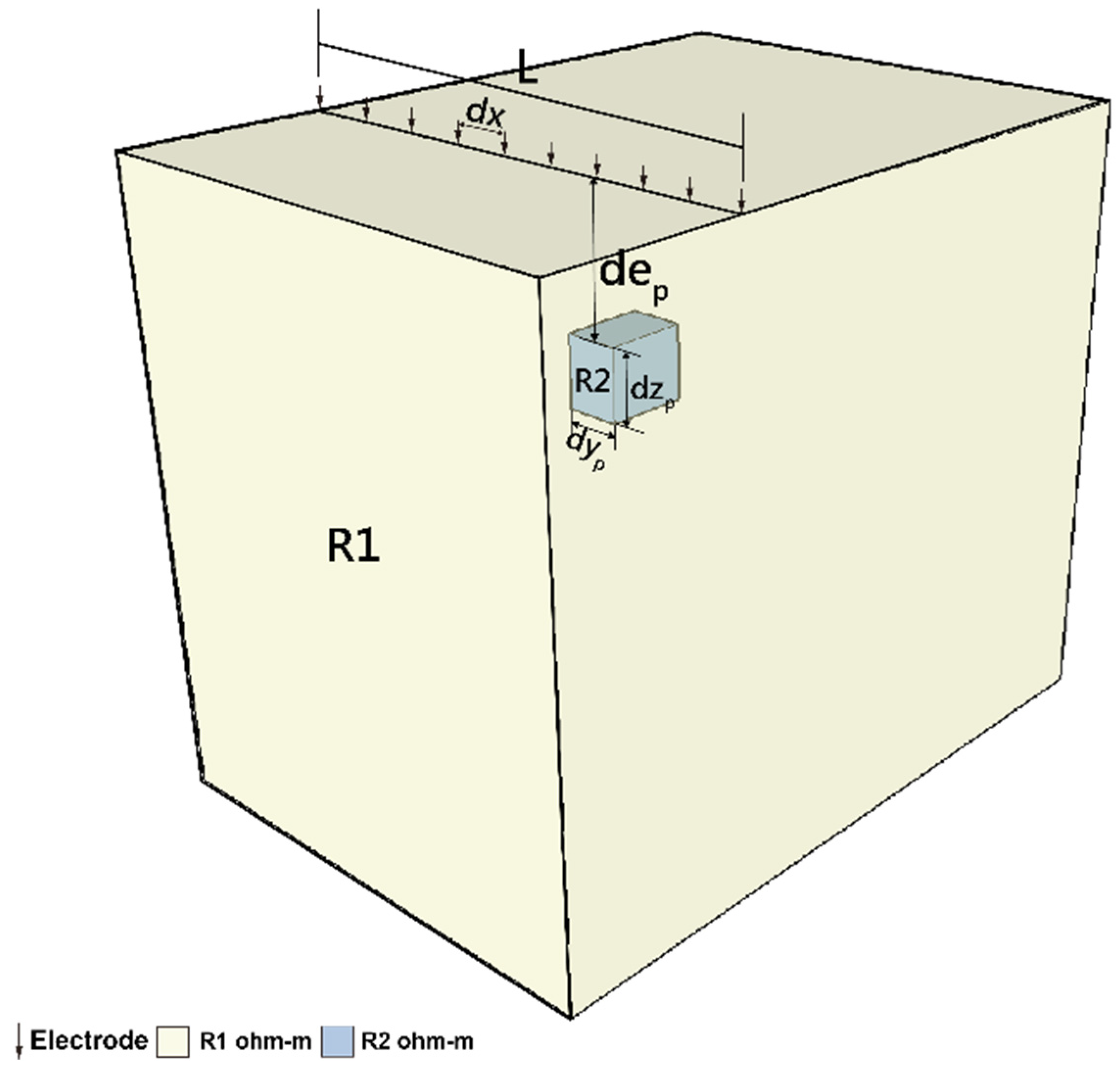
To understand the boundary effect that may be caused by geological formations with pipelines, this study established a geological formation model with pipelines as shown in
Figure 2. This study will establish and plan a geological formation model and testing parameters from the four aspects of resistivity ratio, spacing of the line and pipelines, depth of pipelines building, and pipeline size in the pipelines and strata.
In the model, the resistivity of the pipelines is
R2, the soil layer resistivity is
R1,
R1 >
R2, and the ratio of the two is n (
n =
R2/
R1). To discuss the influence of the resistivity ratio under this assumption, we fixed R1 as 1000 ohm-m, and set R2 as 10, 50, 100, and 250 ohm-m, respectively. The section size of the pipelines was
dyp × dzp, and the depth of the embedding was
dep = 2 m (the top of the pipeline). The parallel pipelines around the pipeline setting were 5 to 6 lines, each line was separated
dy = 3, the spacing to electrode rods was
dx = 3, and each line had a slight adjustment to the length of line L with the sounding requirement.
Table 1 presents the explanatory table of the 3D effect model parameter with the pipeline formation.
3.2. Boundary Effect Model
To understand the boundary effects that may be caused by geological formation changes on both sides of the survey line, this study explored the effects of the boundary effect on 2D ERT through the changes in the boundary medium using numerical simulations by assuming there was heterogeneous media at the boundary. This study explored the influence difference through a model comparison with a boundary effect and no boundary effect, as shown in
Figure 3 and
Figure 4.
The boundary effect was first calculated through the apparent resistivity profile of the model with a boundary medium by forward modeling. Then, we calculated the apparent resistivity by inverse calculation to obtain the resistivity profile of the model affected by the boundary medium. To understand the influence of the boundary effect, this study deleted the data points of the boundary medium in the apparent resistivity profile, and then through recalculation to obtain the new resistivity profile section, we compared the difference between the two. The deleted distances of the data points were 0 m, 2 m, 4 m, 6 m, 8 m, and 10 m from the boundary medium.
This study explored the aspects of the resistivity ratio, electrode spacing, the influence distance of the boundary effect, medium depth, and medium size through parametric variation. In the model, it set that the resistivity of the background soil layer was R1, the resistivity of the boundary medium was
R2, the section size of the medium was
dyp × dzp = 2 × 2 m
2, the embedding depth was
dep = 2 m, the spacing of the electrode rods was
dx = 2, and the length of the survey line was
L = 50 m.
Table 2 is the explanatory table of the boundary effect model parameters.
4. Result and Discussion
4.1. Pipeline Stratum Model under 3D Effect
4.1.1. Resistivity Ratio (n = R2/R1)
To understand the influence of the geological resistivity ratio of the pipeline stratum to the 3D effect, this study set four different kinds of geological resistivity ratio values (n = 0.01, 0.05, 0.1, and 0.25). We fixed the R1 as 1000 ohm-m, and set the R2 as 10, 50, 100, and 250 ohm-m, respectively, for the discussion on the influence of the resistivity ratio.
This study analyzed the influence through small pipeline sizes (1.5 m × 2 m), and the survey line L1~L5 of the small-scale pipeline was sequentially 1.5, 0, 3, 6, and 9 m away from the boundary of the pipeline, therefore, we adopted L3 (where the horizontal distance from the pipeline was 3 m) to analyze. The result of its resistivity ratio is shown in
Figure 5. When the resistivity ratio was less than 0.05, the mapping phenomenon of the 3D effect could be clearly observed, and when the resistivity ratio was more than 0.1, the 3D effect was gradually nonsignificant.
4.1.2. Pipeline Size
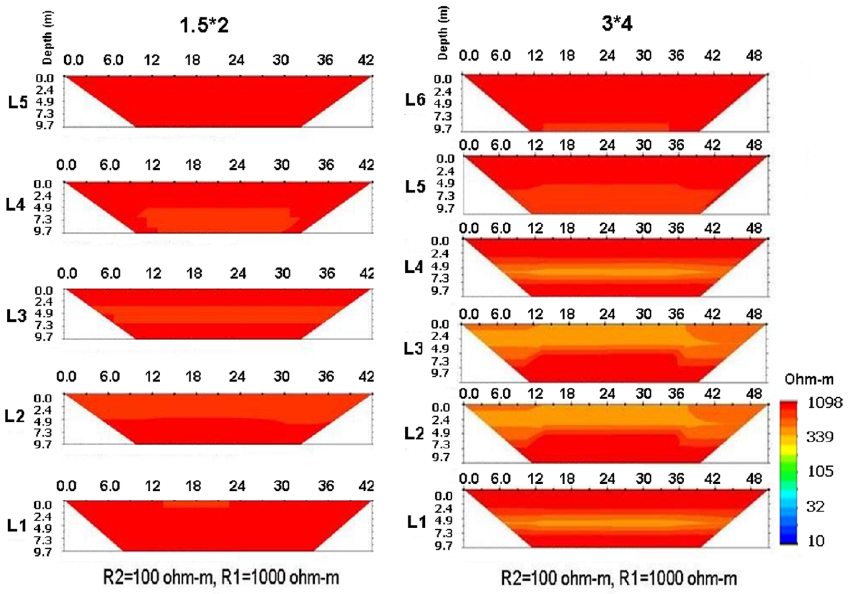
To understand the influence of the pipeline size on the 3D effect, this study set two kinds of stratum models with different pipeline sizes, where the section size of the pipelines was 1.5 (W) × 2 (D) m and 3 (W) × 4 (D) m, respectively. As seen in
Section 4.1.1, when n was more than 0.1, the 3D effect became weaker. Therefore, this study fixed the resistivity ratio to explore the 3D effect under different conditions of pipeline sizes.
Figure 6 shows the results of testing the 2D ERT near two different pipeline sizes. Due to the pipeline sizes, the distances between the L1~L5 lines of the small-scale pipeline and the boundary of the pipeline were 1.5, 0, 3, 6, and 9 m, respectively, and the distances between the L1~L6 lines of the large size pipeline and the boundary of the pipeline were 0 (the left side of the pipeline), 0 (the right side of the pipeline), 3, 6, 9, and 12 m, respectively. In the case of the small pipeline, there was a nonsignificant 3D effect outside the line of the boundary, but in the large size pipeline, line L4 (6 m away from the edge of the pipeline) shows the mapping results of adjacent pipelines. The results show that the influence of the 3D effect increases with the size of the pipeline.
Furthermore, we observed that the mapping depth was deeper than the actual depth of the pipeline. The results showed that the mapping mechanism was not horizontally mapped, and that the mapping depth was related to the distance between the pipeline and the survey line. When the distance was over 6–9 m, the result showed that it was almost unaffected by the 3D effect.
4.1.3. Embedding Depth
To understand the influence of the pipeline embedding depth on the 3D effect, this study set two kinds of models with different depths of embedded pipeline. The embedding depth (the top of the pipeline) was 0 m (embedding at the surface) and 4 m, respectively. The n value in the model was set as 0.1, the section size of the pipeline was 1.5 (W) × 2 (D) m, and there were five survey lines.
Figure 7 shows the 2D ERT results of the small pipeline with an embedding depth of 0 m and 4 m. Compared with the L1 lines (the horizontal distance from the buried pipeline was 1.5 m), when the embedding depth was 2 m, we could obviously observe the mapping phenomena, but when the embedding depth increased to 4 m, the 3D effect was not as obvious. This shows that as the depth increased, the influence of the 3D effect weakened, and the influence range seems to be related to the distance from the line to the pipeline, and not the horizontal distance.
4.1.4. Influence Distance
To find out the possible influence range of the 3D effect in the pipeline stratum, this study used the model that set n as 0.1. The section size of the pipeline was 1.5 (W) × 2 (D) m, dep = 2 m, dy = 3 m, dx = 3 m, L = 42 m, and the L1~L5 lines were 1.5, 0, 3, 6, and 9 m away from the boundary of the pipeline.
As shown in the image on the left in
Figure 7, the profiles at L1 and L3 had a significant 3D effect, whereas the 3D effect of the L4 line profile gradually became less obvious, and in the L5 line profile, there was no 3D effect. Therefore, the 3D effect influence distance was 6 m, and gradually faded after 6 m.
4.1.5. Electrode Spacing
To understand the relationship between the electrode spacing of the pipeline stratum and the 3D effect, and whether the electrode spacing could be used as the normalized parameter, this study analyzed the electrode spacing parameter, which was 3 m and 1.5 m, respectively. The model set n as 0.1, the section size of the pipeline was 1.5 (W) × 2 (D) m, dep = 2 m (the top of the pipeline), dy = 3 m, dx = 1.5 m or 3 m, and L = 42 m.
We used the profiles of L1~L6 to compare the influence situation and influence distance of the 3D effect with different electrode spacings (
dx = 1.5, 3). As shown in
Figure 8, when the electrode spacing was shortened, the spatial resolution improved. However, the influence range of the 3D effect between different electrode spacings was similar; after the distance from the edge of the pipeline increased to 6 m, the 3D effect gradually became inconspicuous. This result shows that it is not appropriate to use electrode spacing as a normalized parameter for the 3D effect because the influence spacing does not decrease as the electrode spacing decreases.
4.2. Boundary Effect Model
4.2.1. Resistivity Ratio (n = R2/R1)
To understand the influence of the boundary effect in different resistivity ratios, this study fixed the background value R1 as 1000 ohm-m, and assumed that the ratio n of R2 and R1 were 0.25, 0.1, 0.05, and 0.01, respectively, that is, the model of R2 resistivity was 250, 100, 50, and 10 ohm-m, respectively.
The results in
Figure 9 show that the presence of the medium in line boundary caused a resistivity profile with an unusual resistivity value near the boundary, and the unusual boundary resistivity value was higher than the background value (1000 ohm-m). The study judged that the current encountered the low resistivity medium in the boundary when it flowed through the boundary. This creates a large amount of current that is concentrated in a low-resistivity zone, and causes the resistivity value of the boundary profile to increase abnormally.
In the case of
n < 1 (
R2/
R1), with the increase in the resistivity ratio value n, the influence of the boundary effect gradually decreased. As shown in
Figure 9, there was an abnormal resistivity value zone in the resistivity profile when the resistivity ratio value n was under 0.1, and was not obvious until the value n reached 0.25. That is, when resistivity ratio is under about 0.1, there are concerns about the boundary effect, which is similar to the situation of the 3D effect.
4.2.2. Medium Size
To understand the influence of the medium size on the boundary effect, this study fixed the electrode spacing and the medium depth, and used the medium size of 2 × 2 m and 4 × 4 m to explore this further.
The results in
Figure 10 show that under the same value n, the addition of the size of the boundary medium does not affect the influence range of the boundary effect; that is, regardless of the size of the boundary medium, the boundary effect is the same, and this situation is different from the 3D effect of the pipeline stratum. It can also be seen in
Figure 10 that the influence ranges of the resistivity ratio
n = 0.1 were the same regardless of the pipe size, and the influence distances were both 8 m.
4.2.3. Embedding Depth
In order to understand the influence of different embedding depths on the boundary effect, this study explored the medium that was 2 m and 4 m under the surface, respectively.
The results in
Figure 11 show that if the boundary medium was the same size, the influence distance of the boundary medium under the surface 4 m was farther than the one under the surface at 2 m. That is, the deeper the boundary medium, the larger the influence of the boundary effect, which is a different situation to that of the 3D effect of the pipeline boundary. It can be seen in
Figure 11 that if the resistivity ratio value n was 1 when
dep = 2 m, the influence distance of the boundary effect was 8 m, and when
dep = 4 m, the influence distance of the boundary effect was 10 m. This result can be seen by the data point of the apparent resistivity in the model; when the medium below the surface is deeper, the deeper data point will be affected, which will cause the influence range of the boundary effect to become wider.
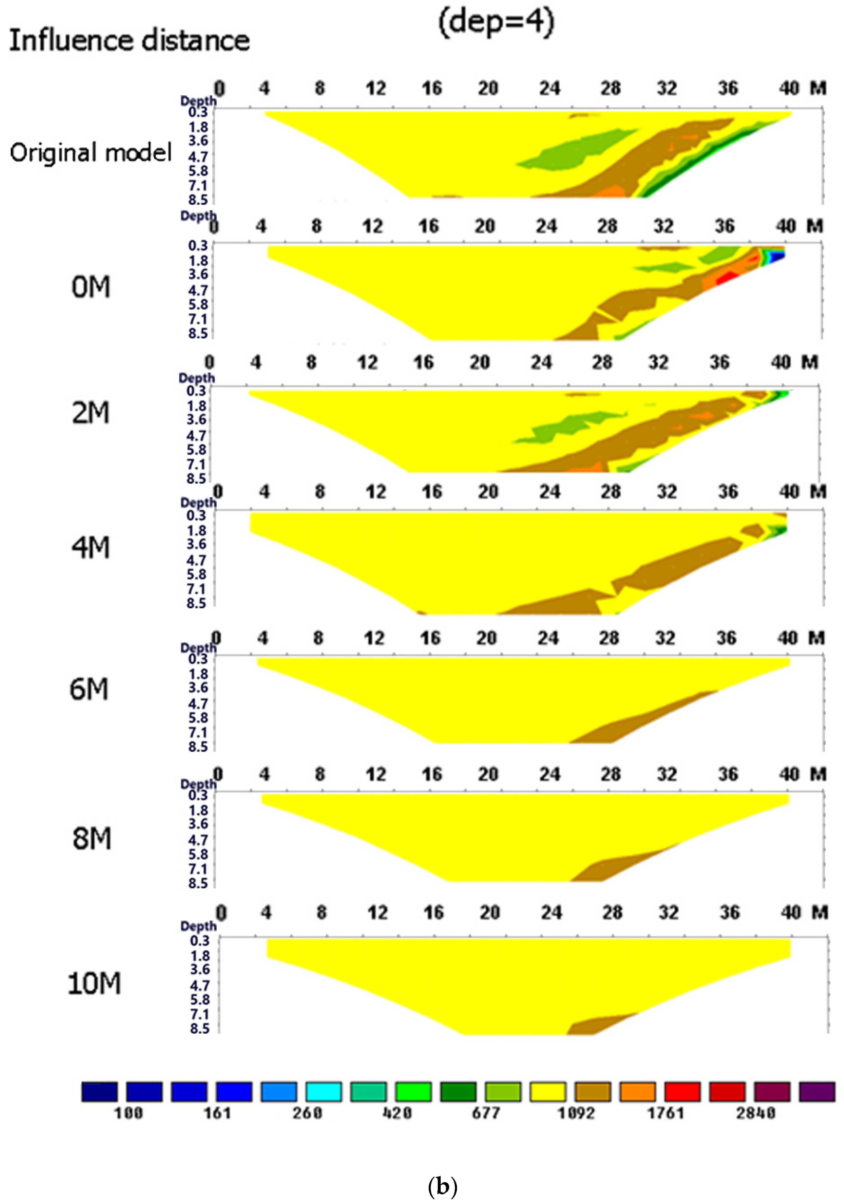
4.2.4. Influence Distance
To understand the influence distance of the boundary effect, this study set the resistivity ratio
n = 0.1 and electrode spacing
dx = 2. These results are shown in the left image in
Figure 12, where the resistivity profile obviously had an abnormal resistivity zone within 6 m from the boundary medium, which was obviously affected by the boundary effect. However, after 8 m away from the boundary medium, it was almost unaffected by the boundary effect. This result is similar to the influence distance of the 3D effect.
4.2.5. Electrode Spacing
To understand the influence between the electrode spacing and the boundary effect, and if the electrode spacing could be a normalization parameter, or whether its effect was a fixed distance regardless of the electrode rod spacing, this study fixed the medium depth and size and set the electrode spacing as 2 m and 4 m, respectively.
When the resistivity ratio value n was 0.1 and the electrode spacing dx was 2, the influence distance of the boundary effect was 8 m; moreover, when the electrode spacing dx was 4, the influence distance of the boundary effect was also 8 m. Although the use of a smaller electrode spacing had better resolution, the influence distances were the same. Therefore, it is not appropriate to use the electrode spacing as the normalization parameter of the influence space of the boundary effect as the influence distance does not become smaller as the electrode spacing becomes smaller. This result is similar to the 3D effect of the pipeline stratum, where neither were affected by the electrode spacing.
4.3. Discussion
2D ERT assumes that the geological formation is a 2D semi-infinite space. However, in the real state of geological formation, the electric current flows in the 3D (X, Y, Z) direction, therefore, the object in the non-2D section has a certain degree of disturbance to the ground resistivity electric field, thus causing some irregular resistivity and noise on the 2D profile [
8], which is called the 3D effect. Many scholars have adopted indoor sandbox experiments to conduct 2D ERT. As a result, a space with boundary constraints is formed. The current transfer is affected by the boundary, and causes some irregular resistivity and noise on the 2D profile, which is called the boundary effect. Most scholars will often choose to evade the 3D effect and boundary effect when performing 2D ERT. Few scholars had made in-depth discussions on the 3D effect and boundary effect. Mei, Xing-Tai used a homogeneous thickness model made from dough to explore the indoor test method and criteria for 2D ERT where. The results of this study and that of Mei, Xing-Tai (2001) both found that the 2D resistivity profile had a boundary effect. Mei, Xing-Tai found that the sandbox experiment needed to have twice the distance of spread to avoid the boundary effect. This study found that the boundary effect had a distance of about 6–8 m. Yang and Lagmanson used a numerical simulation to build a model with three different resistivity blocks, and placed a 2D and 3D survey line on the surface of the model. The results showed that the 2D resistivity profile was mapped by surrounding resistivity blocks and exhibited an irregular resistivity distribution; however, the 3D resistivity profile was not affected [
8]. The results of this study and that by Yang and Lagmanson (2006) both showed that the 2D resistivity profile had a 3D effect. After deeper analysis, the study found that the influence distance was 8–6 m, and that the three-dimensional effect was not obvious after the distance limit of 8 m. Lin et al. conducted 2D ERT at the Hsin-Shan Earth Dam in Taiwan where during the measurements, it was found to be affected by the changes of the nearby stratum and geocenter as well as the curtain grouting wall of the Hsin-Shan Earth Dam, which was at 45 degrees with the survey line. As the 2D resistivity profile had a 3D effect, the authors established the 3D forward modeling of the Hsin-Shan Earth Dam, and compared the differences between the 2D resistivity profile after inverse computing and the Hsin-Shan Earth Dam model. The results showed that the 2D resistivity profile was indeed affected by the 3D effect and had an irregular resistivity distribution [
10]. Both the results of this study and Lin et al. (2013) found that the 2D ERT had a 3D effect. However, the results of this study explored the effects of various influencing factors on the 3D effect and boundary effect in depth, and should be avoided as much as possible in future detection.
In summary, most of the studies that have explored the 3D effect and boundary effect have mostly been to discover and confirm the existence of the 3D effect and boundary effect, or to explore the effects of the 3D effect and boundary effect on a single parameter. As a result, this study explored the effects of the 3D effect and boundary effect on 2D ERT through the parameters of the resistivity ratio, pipeline size, embedding depth, influence distance, and electrode spacing under different conditions and summarized these changes as conclusions and discussed them in detail. In this study, the 3D effect and boundary effect of the 2D resistivity profile were explored through numerical simulation. From the simulation results, good results were obtained, and the relevant results can be used to provide a reference for future detection.
5. Conclusions and Suggestions
ERT can provide the stratum 2D or even 3D resistivity profile to further understand the situation of stratigraphic change, but it is a big challenge to engineer the data interpretation of the ERT spatial resolution and testing result. One important phenomenon in the 3D effect that was observed whilst exploring the pipeline stratum model was the mapping phenomenon of the 3D effect of the pipeline stratum, which will produce an illusion of high and low resistivity in the 2D resistivity profile. The boundary effect will cause the resistivity value of the 2D profile boundary to abnormally increase, reduce resolution, and increase interpretation error. Through the model established in this study, it was found that there was roughly similar influence trend in the parameter analysis of the 3D and boundary effects. The following are suggestions for future testing.
Under different resistivity ratios (n), when the n value increases (that is, the difference in resistivity between the formation and the medium becomes smaller), the influence ranges of the 3D and boundary effects both decrease.
The 3D and boundary effects have a similar influence range, with an influence distance of 6~8 m.
Different electrode spacings showed that it is not appropriate to use electrode spacing as a normalization parameter because the influence distance does not increase as the electrode spacing increases.
With different medium sizes, an increase in the pipeline size will increase the range of the 3D effect, but the boundary effect is not affected by the size of the medium.
At different embedding depths, the deeper the buried depth, the smaller the 3D effect of the pipeline, but the greater the boundary effect of the medium. This is because the deeper the boundary medium, the more the resistivity changes at the deeper boundary profile.
Currently, the scope of this study is only to establish a numerical model. In the future, we will try to confirm the results of the numerical simulation through in situ testing.


