Article

Distribution of PM2.5 Air Pollution in Mexico City: Spatial Analysis with Land-Use Regression Model

1
Antropo SIG CIESAS, Calle Juárez No. 87, Tlalpan 14000, Ciudad de México, Mexico
2
Department of Electromechanical Instrumentation, Instituto Nacional de Cardiología Ignacio Chávez, Juan Badiano No. 1 Col. Sección XVI, Tlalpan 14080, Ciudad de México, Mexico
3
Department of Sociomedical Research, Instituto Nacional de Cardiología Ignacio Chávez, Juan Badiano No. 1 Col. Sección XVI, Tlalpan 14080, Ciudad de México, Mexico
*
Author to whom correspondence should be addressed.
Appl. Sci. 2019, 9(14), 2936; https://doi.org/10.3390/app9142936
Submission received: 9 June 2019 / Revised: 8 July 2019 / Accepted: 18 July 2019 / Published: 23 July 2019
(This article belongs to the Special Issue Air Pollution)

Abstract

:

Featured Application

Modeling the spatial distribution of PM2.5 with personal monitors and an LUR approach may be useful for local authorities to make accountable public policy decisions.

Abstract

In this study, the spatial distribution of PM2.5 air pollution in Mexico City from 37 personal exposures was modeled. Meteorological, demographic, geographic, and social data were also included. Geographic information systems (GIS), spatial analysis, and Land-Use Regression (LUR) were used to generate the final predictive model and the spatial distribution map which revealed two areas with very high concentrations (up to 109.3 µg/m3) and two more with lower concentrations (between 72 to 86.5 µg/m3) (p < 0.05). These results illustrate an overview trend of PM2.5 in relation to human activity during the studied periods in Mexico City and show a general approach to understanding the spatial variability of PM2.5.

Graphical Abstract

1. Introduction

Air pollution is a well-known health problem affecting several mega cities, especially those in low- and middle-income countries where more than 80% of the population is exposed to dangerous air quality levels, which frequently exceed the World Health Organization’s (WHO) air pollution guideline limits [1].
Human exposure to air pollution is a major concern due to the related health effects, especially when the pollutant in question is PM2.5, since it can originate from different sources at various sites with a composition of a wide variety of chemical substances [2].
In Mexico City (formerly Distrito Federal), there is a severe air pollution problem due to the presence of several diverse factors: (a) its geographical situation in the lacustrine plain of an endorheic basin [3]; (b) its average altitude of 2240 m above sea level (masl) in its central part; (c) it is surrounded by mountains with an average height of 1000 m above the basin level; and (d) unpredictable but frequent meteorological phenomena that affect the environment (e.g., volcanic ash clouds, hurricanes, droughts, floods, wildfires). Furthermore, (e) its demography aggravates the problem with its 16 boroughs (geographical and governmental units within Mexico City) with an uneven population density [4]; (f) the overpopulation phenomenon has increased the number of automobiles by more than three times—from 1,869,808 in 1980 to 5,725,574 in 2016—thus incrementing traffic and also the sources of PM2.5 pollutants [5] (Figure 1).
Several measures have been taken since 1990 to deal with the air pollution problem in Mexico City: compulsory use of catalytic converters, introduction of unleaded fuel [6], the recent creation of the Environmental Commission for the Megalopolis (Comisión Ambiental para la Metropolis CAMe) [7], and a new regulation on PM2.5 [8]. Nevertheless, ten environmental contingencies were registered in 2016 [9]. The first epidemiological studies evaluating health problems related to air pollution in Mexico City [10,11,12,13] were made with ambient monitors. More recently, studies have been carried out following a personal monitoring method [14,15]; PM2.5 started to be measured in some stations of Mexico City’s automatic air quality monitoring network (Red Automática de Monitoreo Atmosférico, or RAMA) in 2004 [16].
Land-use regression (LUR) models developed by Briggs [17] have been successful in describing the spatial variations of pollutants. They also offer more advantages than other approaches because of the statistical relation between the pollutant concentration and the sites where pollutants are monitored, which could also be established with other factors such as population density, traffic, altitude, and weather conditions, amongst other aspects. This analysis has been used in Europe [18,19] and the United States to model air pollution exposure [20,21] and, more recently, in Asian and Middle Eastern countries like China [22,23], Iran [24], and India [25]. However, it has never been used in Mexico City.
There is plenty of scientific information regarding air pollution problems in Mexico City; nonetheless, inhabitants’ personal exposure to PM2.5 air pollution has yet to be evaluated. Land-use regression models have been used to analyze air pollution spatial distribution using ambient monitors, although inhabitants’ exposure may still be questionable [25,26]. Land-use regression models have also been estimated with personal measurements of air pollution which could be better indicators of exposure since the analysis includes information about the inhabitants’ daily activities related to sources of air pollution in indoor environments [19,27].
The purpose of this study was to model the spatial distribution of PM2.5 air pollution with personal measurements of PM2.5 using Geographic Information Systems (GIS), a land-use regression approach, and indirect measurements of road speed limits (RSLs), as well as population density, weather conditions, topographic characteristics, and the Normalized Difference Vegetation Index (NDVI) [28].

2. Materials and Methods

2.1. Participants and Meteorological Variables

The study was carried out between April and August 2002. Thirty-seven participants were included their personal exposure monitors to PM2.5 were used, and they represented the first measurement of PM2.5 air pollution in Mexico City. Exposure was measured using a pDR nephelometer calibrated according to technical information [29].
Personal exposure periods were selected if the address was available and had a duration of at least 1 and half hours, then by means of participants’ written diaries. PM2.5 exposure periods were classified as “daytime” from 11:00 to 12:30, and included 12 measurements, whereas those between 21:30 and 23:00 were classified as “nighttime” and included 25 measurements. Moreover, measurements were also classified as within indoor or outdoor microenvironments in 30 min periods, thus, home or office addresses were geo-localized as described below. No measurements were taken during weekends. All participants lived in Mexico City in 13 of the 16 boroughs (see Figure 1). A detailed specification of the equipment and the sampling method utilized in this research have been published elsewhere [30].
Average annual measurements of meteorological variables, such as relative humidity (RH, %), temperature (TEMP, °C), wind speed (WSP, m/s), and wind direction (WDR, the azimuth direction from which it originates) were taken from the meteorological network stations [31] located in the areas closest to the participants’ addresses (distribution by geographical location of annual average relative humidity and temperature is shown in Supplementary Materials Figure S1). Since pDR measurements can be biased with an RH above 70%, the information was double-checked on the days PM2.5 was measured and RH was lower than 70% according to RAMA [32,33,34]. Several measurements were close to each other; thus, the median was calculated to improve the locations and reduce the sample redundancy.
Weather conditions and PM2.5 personal measurements were compared between daytime and nighttime and simultaneously among geographical locations. A non-parametric method was used (Friedman test) since data distribution was different from the normal standard (Shapiro–Wilks p < 0.05). Data are presented as median (interquartile range (IQR)). Statistical significance was considered with a p-value > 0.05.

2.2. Geographic Information System

The PM2.5 personal exposure data were placed into a database containing the address of each participant where the samples were taken; the coordinates of these locations were obtained using Google Earth geocoding. With this database, each pair of coordinates was transformed into a point using ArcGIS 10 [35]; subsequently, a series of interpolated surfaces was generated with the extension Geostatistical Analyst and Spatial Analyst.

2.3. Raster Data and Interpolation

Annual average values of RH, WDR, WSP, and TEMP were interpolated using the Inverse Distance Weighting (IDW) method [36,37]; the resulting maps were standardized using a pixel resolution of 500 m. A smooth surface was needed along with the preservation of the original average values. According to the Red de Meteorología y Radiación Solar (REDMET), the stations are strategically distributed across the basin; therefore, the distribution of points and the distance between them were expected to be even (geographical location of the REDMET stations are provided in Supplementary Materials Figure S1). Inverse distance weighting (IDW) assumes that each measured point has a local influence that diminishes with distance. It gives greater weights to points closest to the predicted location, and weights decline as a function of distance [36,37]. This principle fits perfectly with this kind of data since what was sought was not the identification of a trend, but a continuous hypothetical surface based on the accumulated average values throughout a year.
An interpolated surface was generated specifically for PM2.5 to create the dependent variable map. We created a simple IDW interpolation just to show the raw values of PM2.5 graphically. Nonetheless, an ordinary kriging interpolation method was used for analysis. Kriging has been tested several times to measure its reliability as a predictor and can accurately predict unknown values of a limited sample when contrasted to a set of known values, especially when the samples are randomly distributed [36,38,39,40]. Kriging assumes stationary data, as in “the condition that the probability of distribution of the variable is constant in time and/or space, meaning that the same function of distribution probability could be expected anywhere and anytime” [41]. Due to the uniform distribution of the particulate matter, it was presumed to be stationary since the sources of pollution are located in fixed places, namely, roads, factories, houses, and public places. Therefore, the function probability of these variables withholds its properties [42]. For example, it is more likely for the surrounding area of a factory to be more contaminated than a place far away from it, which is the underlying approach of autocorrelation. Accordingly, an interpolated map was produced using the 37 PM2.5 samples; in order to generate a better understanding of the spatial variability in PM2.5, if a particular point had two different measurements (day or night), it was decided to use the one with the highest value of PM2.5. It has been noticed that high values of ambient PM2.5 concentrations do not necessarily reflect peaks of exposure [26,43,44]. We wanted to capture these high values, measured per personal monitor, to consider a hypothetical and possible acute toxic effect for further focused research.
The nature of PM2.5 implies the use of anthropogenic and topographic data to evaluate the relationship between the particles and the location of human activities [45]. It was assumed that the higher the RSL, the higher the values of PM2.5 in the surrounding areas would be due to the way traffic behaves [45]. Therefore, road line data were used to approximately reflect this variation and produce a continuous surface for the RSL [4]. The lines of the roads were transformed into points separated every 250 m, which were then interpolated using IDW with a resolution of 500 m. Hence, buffered zones of the average speed value were used rather than fixed values. In the case of population density (PD), the 2005 census was used [46] in addition to the electoral sections (Geoelectoral Census Statistics) Estadísticas Censales a Escala Geoelectoral [46], since these were the most accurate sources available that fulfilled our purpose. The centroid of each electoral section was extracted and given the value of each polygon; then, an IDW interpolation was performed. Inverse distance weighting as used to reflect data fuzziness due to the discrete nature of roads and districts.
The digital elevation model, which had already been interpolated from the original Shuttle Radar Topography Mission (SRTM) source [47], was resampled to fit the 500 m resolution and used to produce the slope and aspect maps. A map was created showing the incidence of wind over a surface (WIOS); it combined the wind direction and the aspect maps since the values of the former were in degrees and continuous data were needed to achieve better results with the canonical analysis. A raster file was created to detect the incidence of the wind (wind direction) over a particular surface (aspect). The windwards and leewards were identified and assigned a value depending on the angle of incidence of the wind in contraposition to the aspect:
(a)
A value of 0 meant that the wind ran in the same direction of the surface (leeward). Concerning the contaminants, no deposits were assumed.
(b)
A value of 1 meant that the angle of incidence of the wind according to the surface was parallel and there could be either erosion or deposition.
(c)
A value of 2 meant that wind impacted on the surface at angles between 30 and 60 degrees; that is, oblique. High deposits and less erosion were expected.
(d)
A value of 3 meant that the wind impacted the surface perpendicularly, that is, in angles, close or equal to 90 degrees (windward). It was considered a surface where the possibility of high deposition of contaminants exists. (Detailed information on the geographic, demographic, and meteorological variables used is provided in Supplementary Materials Table S1).

2.4. Multivariate Analysis

A matrix of the product–moment correlation coefficient (Pearson’s) was created to identify which variables were correlated, as in how much of the variance was shared among them; those with the strongest correlation coefficients (more than ±0.4) were separated into two groups. Due to the geographical, social or meteorological conditions, in some cases, it was better to keep them together even if they were highly correlated (e.g., slope and temperature) (the Pearson’s correlation coefficients are detailed in Supplementary Materials Table S2). This analysis helped us to decide how to arrange variables for the canonical correlation analysis. The RSL was included even though its correlation coefficient was lower than 0.40 because of the well-known relationship with PM2.5 air pollution [45].
The canonical correlation analysis correlates simultaneously with both metric and non-metric variables. Its strength relies on the possibility to correlate two sets of variables. Canonical correlation analysis facilitates the study of linear interrelationships among two sets of variables [48].
In this case, the first set of canonical variables were altitude, RH, NDVI, WIOS, and WSP (p) (X1, X2, … Xp), and the second set of variables were PD, slope, TEMP, and RSL (q) (Y1, Y2 … Yq).
The main objective of canonical correlation is to identify the r lineal combinations within the first variables.
U1 = a11X1 + a12X2 + … + a1pXp
U2 = a21X1 + a22X2 + … + a2pXp
Ur = ar1X1 + ar2X2 + … + arpXp
and within the second variables:
V1 = b11Y1 + b12Y2 + … + b1qYq
V2 = b21Y1 + b22Y2 + … + b2qYq
Vr = br1Y1 + br2Y2 + … + brqYq
The most significant correlation coefficient will be shown between U1 and V1. The second one will be between U2 and V2 under the condition that there is no correlation between U1 and U2, and between V1 and V2. Finally, the third most significant correlation will be shown between U3 and V3 and, as previously mentioned, there should be no correlation between U3 and U1 and U2, and between V3 and V1 and V2. These combinations are called the canonical variables.
The raw canonical coefficients, which define the linear relationship among the variables, can be interpreted in the same way as regression coefficients [49], so they were used to create a predictive surface to identify where the occurrence of contaminated sites was more likely to occur. The aim was to know the effect that the estimated linear coefficients of the proposed variables have over each other, thus providing a general adjustment (canonical coefficients are detailed in Supplementary Materials Table S3).
Geographic Resources Analysis Support System-Geographic Information System (GRASS GIS) [50] was used to create the predictive surface and to produce a series of cross-tabulate tables (r.stats module) among all the predictors using data points from personal PM2.5 exposures.
The predictive surface map was created using map algebra, where each linear coefficient from the canonical model multiplies its related predictor variable using a simple linear predictor function f(i), which is the final estimation resulting from the combination of the predictor variables and the PM2.5 concentration:
f ( i ) = β 0 + β 1 x i 1 + . + β p x i p + e
where β0 is the intersection that, in this case, is the value of the concentrations of PM2.5 in the interpolated surface; 1 … p are the linear coefficients of the canonical correlation analysis indicating the relative effect of a particular predictor on the outcome [49]. For instance, if the predictor variable was the RH, then each interpolated pixel with a given value for RH was multiplied by its own coefficient.
In order to have an estimated value of PM2.5 driven from the linear function used for the construction of the map of the spatial distribution of PM2.5, normalized values were calculated with the largest concentrations of PM2.5 obtained from the kriging interpolation (122.4040) and from the linear function of the multivariate analysis (109.64) with the following formula:
Normalized   values   of   PM 2.5 = ( 122.4040   ×   Values   of   PM 2.5   estimated   by   the   linear   function ) 109.64
The internal validity of the final predictive surface was tested first by generating a cross tabulation to extract the raster values from the Ordinary Kriging model; then, the RMS of the adjusted model and the residual error were estimated. Performance between original samples, ordinary kriging estimates, and fitted values from the predicted surface were evaluated with Boostrap and K-fold cross validations.

3. Results

3.1. Comparison of the Ambient Distribution of Meteorological Variables and PM2.5 Air Pollution within Each Borough between Day and Night

Annual average RH and TEMP are shown in Supplementary Materials Figure S1. Relative humidity (RH) as well as TEMP obeyed seasonal variations during the year. Relative humidity showed minor variations throughout Mexico City’s territory; however, it was lower during the dry season, rising up to 99% during the rainy season. The TEMP had similar behavior, with temperatures relatively constant along the year with small variations (14 to 16 °C); however, for some days during the winter, temperatures could drop to 0 °C or rise up to 31 °C during the spring.
Regarding the wind, its predominant direction (WDR) was from north to south/southeast. Yet, another pattern was identified from north and northwest where the winds seemed to blow towards the northeast. In the south, the wind’s direction was also from north to south. Average wind speed (WSP) along the year was relatively constant, ranging from 0.0019 to 3.72 m/s depending on the season (graphical information on wind direction is provided in Supplementary Materials Figure S2).
Throughout the period of this study, fewer variations were identified apart from the obvious differences in the weather conditions between day and night. In general, nights were more humid (RH 71.1% (65.5–79.9%)) and cooler (TEMP 16.3 °C (14.8–16.8 °C)) than days (RH 54.1% (45.4–61.3%) and TEMP 19.7 °C (18.3–21.1 °C)). The WSP varied more during the night (1.5 m/s (0.95–2.3 m/s)) than during the day (1.2 m/s (1.1–1.5 m/s)) (detailed information on the weather conditions by geographical distribution between days and nights is provided in Supplementary Materials Table S4).
No meaningful differences were observed in relation to TEMP and RH by geographical location; however, the most humid area during both day and night was the southeast (day: 62.4% (51.9–63.4%), night: (76.7% (68.5–81%) (p = NS)). The WSP showed no significant differences, neither geographically nor between day and night (detailed information on the weather conditions by geographical distribution between days and nights is provided in Supplementary Materials Table S4).
The PM2.5 personal measurements obtained in this study are shown in Figure 2. During daytime, concentrations of PM2.5 were above national standards for the year 2002 (65 µg/m3)—the current national standard is 45 µg/m3 in the 13 boroughs [8]. The highest levels of PM2.5 were identified in Cuauhtémoc (180 µg/m3), Benito Juarez (108 µg/m3 (69–160 µg/m3)), and Miguel Hidalgo (118 µg/m3) in the center of the city, and Azcapotzalco (112 µg/m3), which is located in the north part of the city. Incidentally, there was a gap between the city center and the eastern area, with low concentrations that incremented in the center of Iztapalapa (133 µg/m3), which is a borough in the southeast part of the city. The lowest concentrations were observed in the boroughs of Coyoacan (66 (63–69 µg/m3)) and Magdalena Contreras (77 µg/m3), located in the southwest (Figure 2A).
During the night, PM2.5 median concentrations throughout Mexico City were lower than during the day; the highest median concentrations were detected in Tlalpan (96 µg/m3 (64–118 µg/m3)) in the south of the city, and in Iztacalco (87 µg/m3) in the center; followed by Coyoacan (63 µg/m3 (27–74 µg/m3)) in the southwest, and Cuauhtémoc (59 µg/m3 (55–62 µg/m3)) in the center. The lowest PM2.5 concentrations were registered in the southeast in Xochimilco (37 µg/m3) and in the southwest in Magdalena Contreras (26 µg/m3) (Figure 2B).
Meaningful differences in PM2.5 concentrations were detected among boroughs, despite the differences observed between day (94 µg/m3 (73–126 µg/m3)) and night (49 µg/m3 (39–74 µg/m3) (p = 0.0006)) (detailed information is provided in Supplementary Materials Table S4).

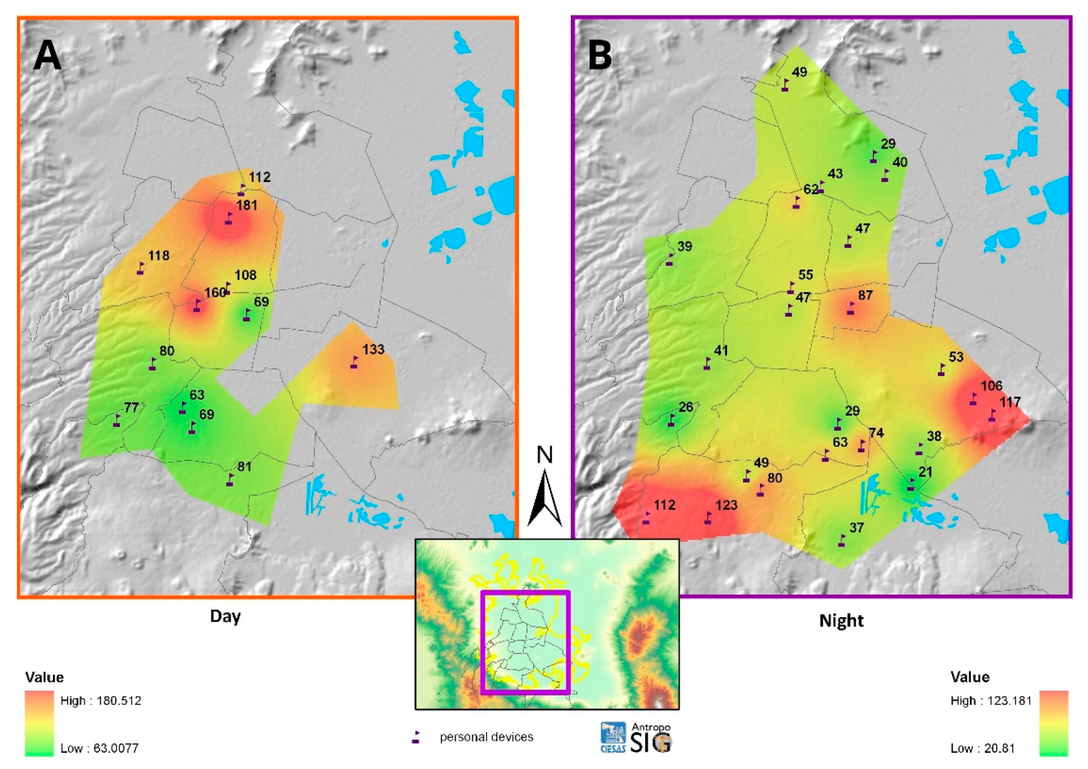
3.2. Spatial Distribution of PM2.5

The spatial distribution of PM2.5 is represented in Figure 3, where personal monitor measurements of PM2.5 were used as the dependent variable. The map resulting from the LUR model shows four areas with different spatial distributions of PM2.5. The first and largest one is represented by a diagonal running from the northwest to east, covering six boroughs: Azcapotzalco, Miguel Hidalgo, Cuauhtemoc, Benito Juarez, Iztacalco, and Iztapalapa. In this area, the median concentration of normalized PM2.5 was 79.1 µg/m3 with an interquartile range between 67.1 to 89.9 µg/m3.
The second area is situated in the southwest part of the basin, in the boroughs of Tlalpan and Magdalena Contreras. Since the latter is a transition area between the two boroughs, the median concentration of normalized PM2.5 was only approximately 78.2 µg/m3 with an interquartile range 67.8 to 104.1 µg/m3.
The third area runs from the northeast in the borough Gustavo A. Madero, crosses Cuauhtemoc in the center, and ends in Venustiano Carranza, which is located in the northeastern part of the basin; in this case, the median concentration of normalized PM2.5 was 47.5 µg/m3 with an interquartile range between 39.5 to 48 µg/m3.
The fourth and last area was in the southwestern part of the basin, and covered the southern areas of Coyoacan and Iztapalapa, plus the northern part of Xochimilco. The median concentration of normalized PM2.5 was 60.6 µg/m3 with an interquartile range between 51 to 68.6 µg/m3.
The first and second areas showed the largest concentrations of normalized PM2.5 in Magdalena Contreras, Cuauhtemoc, and Azcapotzalco (78.1 µg/m3 (two measurements with the same values) 81.8 µg/m3 (75.4–103.4 µg/m3), and 90.7 µg/m3 (one measurement), respectively); whereas, the lowest concentrations were observed in the third area, more precisely in Gustavo A. Madero and Venustiano Carranza (43.5 µg/m3 (35.2–47.7 µg/m3), 58.8 µg/m3 (one measurement), respectively). Finally, it is important to outline the overestimation identified in the concentration of PM2.5 in the normalized values when compared to the personal measurements originally taken (Table 1).
Post-processed data showed a reasonable estimate of prediction. The RMS from the fitted model (38.94641) and from the residual error (38.03686) differed only by 2.2% (standardized RMS = 1.022); the validity of Kriging interpolation through Bootstrap and K-fold cross performed similar to that of the predictive surface. Therefore, both the interpolation method and the adjusted interpolated method using the fitted variables were reliable.

4. Discussion

This is the first study of a PM2.5 spatial modeling distribution made in Mexico City with personal monitors and with an LUR approach, even though the sampled data were from the year 2002. We considered that it was important to show how inhabitants are exposed to high levels of PM2.5 at the personal level, that air pollution varies throughout Mexico City, and that environmental conditions then and at present remain far from optimal. As a matter of fact, ten environmental contingencies were recorded just in 2016 [9] despite the new regulatory limits for PM2.5 air pollution [8] and the creation of the Environmental Commission of the Megalopolis (Comisión Ambiental para la Megalópolis, CAMe) [7,51].
Several studies have tried to understand the occurrence of air pollution by using a holistic model, where a broad-spectrum of variables tackled the complex dynamism of larger cities. An LUR model can be used as an alternative approach to a dispersion model, and it allows to obtain a statistical relationship between land use characteristics and pollutant concentrations measured through sampling at a limited number of sites. The relationship is used to predict pollutant concentrations at unmeasured locations throughout a given domain [25].
Even when the LUR model allows to integrate geographic, topographic, social, and environmental variables altogether to evaluate the effect of one or more atmospheric pollutants, the criteria for including specific variables into the model could be as diverse as the city itself [18]. In general, the demographics, as well as the environmental conditions, are considered when the authors indicate that they used LUR. The use of road and traffic information to deploy the analysis is also typical [52,53,54,55,56]. The richness of this approach is its versatility; therefore, the uses of variables and the ways in which they are correlated are not determined [57]. An estimate of the adjustment for all other variables included in the LUR model with their respective canonical weight will be provided by using the canonical correlation to estimate the covariance of these variables.
This study documented the use of an LUR model involving the use of GIS for the construction of map layers and linear statistical methods to estimate the exposure in which predictor variables were selected and obtained from different sources such as population density, RSL, topography, weather conditions, and personal monitor samples of PM2.5 concentrations. Contaminants’ dynamics were determined by meteorological variables; yet, their distribution among complex urbanscapes like Mexico City should be understood considering geography, urban and social characteristics.
This study also shows that some pollution emission sources tend to be located along main roads or places that are highly frequented due to the fact of a certain mobility paradigm, interconnection nodes, supply and financial centers or public services, making them relatively stationary [58]. Thus, roads were considered as an indirect and dynamic type of a stationary pollution emission source related to primary nodes and peak hours.
The use of personal monitors to estimate population exposure is crucial since they are the only tools that could sample the variability of air quality to which people are exposed. Personal monitors allow to take samples at the human scale whenever necessary, and hypothetically, we could sample this complexity either in indoor environments such as homes, offices, and schools, or outdoors such as along the road, on the bus, in the middle of a park, next to a factory, and so forth. Additionally, it is important to consider that people spend most of their time in indoor environments which have their own sources of contaminants [59]. Recent studies have found that personal exposure is higher than those measured in fixed sites [23,60] and that it is determined by people’s activities, especially in indoor environments [27,61]. This study showed that the spatial distribution of PM2.5 identified two areas in which PM2.5 levels were very high, and two more with lower ones; these areas were distant from each other, with very different social, economic, and topographic conditions, where local stratified sampling methods might be used in further studies.
When the variables were chosen, we expected to find a spatial relationship among them, as well as between their locations and interactions [62]. The basin of Mexico is not a flat surface with standard meteorological and topographical conditions; it is neither homogenous in its social, economic, commercial, and transport networks. On the contrary, the city is a mixture of micro-environments entangled within an intricate collection of geomorphological features in which conditions can change from one place to another, including the induced biological effects caused by a different composition of the particulate matter [63,64].
The results showed how the abovementioned conditions might influence the spatial distribution of contaminants such as PM2.5. For instance, the spatial distribution of PM2.5 was the lowest in the northern area of Xochimilco, located in the south part of the basin (Figure 1, borough 13), which is well known for its chinampas (part of the UNESCO’s list of human heritage). This area is one of the least contaminated regions in the city. This could be related to the high levels of humidity due to the amount of lakes, canals, and trees. This region presented some of the highest continuous NDVI indexes in the study area (approximately 174 ha with an index value of more than 0.3, just in the wetlands with a maximum of 0.489). Furthermore, this borough is in some ways protected by the Iztapalapa peninsula and the Huizachtecatl volcano, which serve as a wall that impedes the free flow of wind from north to south. Moreover, most of the population is located on a flat surface that is interrupted by the piedmont of the volcanic field of the Sierra Chichinautzin; therefore, the dispersion of contaminants could be more efficient and the region cleaner.
It is worth mentioning that the spatial distribution of PM2.5 was higher in other areas. For instance, the spatial distribution of PM2.5 was among the highest in the borough of Iztapalapa, located in the southeast part of the basin (Figure 1, borough 7) (Figure 3). This does not come as a surprise since the borough has intrinsic characteristics such as its high population density (Instituto de Vivienda del Distrito Federal, Comisión Nacional de Fomento a la Vivienda, & Universidad Autónoma Metropolitana, 2007) and its particular topography consisting of a small mountain formation called Iztapalapa Peninsula. This formation extends all the way to the Santa Catalina range. The Huizachtecatl volcano, or the Star mountain, is located almost in the center of the borough. As previously said, these three formations range from 2400 to 2900 masl and constitute a natural wall that prevents the wind from flowing from north to south. Therefore, it is possible for the wind to deposit the pollution at the north facing slope of these topographical formations. The Central de Abasto (Supply Center) is also located in Iztapalapa, north of these mountains, and is one of the busiest places in the whole country. According to the Supply Center webpage [65], this market distributes up to 35% of fruits and vegetables in the country, handles over 30,000 tons of merchandise per day, is attended by more than 500,000 people per day, and has 62,000 vehicles in transit within its borders.
The spatial distribution of PM2.5 in the western and northwestern parts of the basin was the highest (Figure 3). This region had relatively high levels of humidity related mainly to the Chapultepec Park, located in Miguel Hidalgo (Figure 1, borough 16), where the NDVI ranges from 0 to 0.2, the population density is low and there is a relatively large density of trees. The boroughs in this region are considered some of the wealthiest within the city. However, the area is composed of a mixture of at least three major commercial–touristic–business corridors that lack a proper and efficient public transportation system to support the mobility of all the people that operate in this area. Most of the workers drive to work during peak hours, causing traffic jams and delaying people coming from the eastern part of the city, who have to drive for at least two hours to get to work or home. The privation of a sustainable and well-planned urban development program has generated a gentrification problem that results in the excessive use of cars, destruction of green areas, the construction of skyscrapers, shopping malls, residential buildings, parking lots, and toll highways that expel low-income residents to slum areas [66]. This excessive urbanization process has contributed to a temperature increment of 0.39 °C per decade in Mexico City [67,68,69,70].
Another surprising result was the very high spatial distribution of PM2.5 found in Tlalpan (Figure 3), located in the southwestern part of the basin (Figure 1, Borough 12). It is the second largest borough in Mexico City with a total surface of 312 km2 (20.7% of Mexico City’s total area). Tlalpan also has the lowest population density (1878 inhabitants per square kilometer), and it is considered one of the main “lungs” of the entire basin since it is one of the most extensively forested areas of Mexico City. Due to the presence of geological features and the amounts of rainfall, Tlalpan is an important hydrological deposit area of the city. It has a large surface that is protected by the legal entities of Land Conservation and Natural Protected Areas [71], which aims to preserve, restore, and reforest the area to maintain the ecological balance not only within the borough but the whole basin. However, some peculiarities could increase the spatial distribution of PM2.5 in Tlalpan. On the one hand, the population density is irregular, with urban communities in the north, and suburban and rural communities in the south, all mixed among healthy vegetation areas (NDVI ranges from −0.39 to 0.58, and about 94 ha with an index of more than 0.3). On the other hand, the wind flow tends to go from north to south in the basin (Figure 3), making this area potentially risky. In the afternoon, all the contaminants are transported to the south and deposited on the piedmont of the Chichinautzin mountain range, where they are slowed down by the increment in humidity and the decrement in temperature. A strong correlation between the particulate matter and the windward was observed, which suggests that in the south/southwest region of the basin, the spatial distribution of PM2.5 is higher during the afternoon than during the night due to the dispersion and deposition processes.

5. Study Limitations

The sample size used in this study can be considered somewhat small. Kriging interpolation was used to overcome this limitation since it is a well-known method to accurately predict unknown values from a limited sample [36,38,39,40].
The occupational composition distribution of the sample was simple and balanced and failed to represent that of the study area. Ideally, however, and not possible for this study, a stratified systematic sampling method should be used to represent the variability of activities—spatially and temporally—in the city, monitoring individuals 24/7 from different strata (activity and region) during an entire year. However, the evaluation of the occupational exposure goes beyond the purpose of this study.
Statistical modelling was based on PM2.5 personal exposure, whereas meteorological conditions were taken from ambient monitors; however, environmental variables showed an important correlation between outdoor and indoor environments. In fact, most epidemiological studies of PM2.5 air pollution have relied on measurements taken by ambient monitors. Furthermore, outdoor weather conditions—air temperature and relative humidity—might influence indoor environments, but also housing characteristics such as the integrity of a building’s envelope, state of mechanical heating, ventilation and air conditioning systems can modify indoor microenvironments [72]. Several studies have demonstrated that outdoor temperatures highly correlate with indoor ones [72,73,74]. Temperature and relative humidity are tightly correlated; the combination of both is used as an index (humidex) that reflects the perceived temperature. Both temperature and relative humidity can vary widely depending on the location and the season [72].

6. Conclusions

Most of Mexico City´s dwellers live in an unhealthy atmosphere because of the unplanned urbanization process, over-population, increasing vehicle fleet, and the scarcity of green areas in the city. The holistic analytic approach using LUR models allows the integration of variables with an atypical behavior into a dispersion model that could better explain the patterns of exposure to PM2.5 air pollution. Even though more studies are needed to deepen the investigation of the exposure to PM2.5 air pollution patterns of Mexico City’s residents, the results presented here could help local authorities make accountable decisions on the inhabitants’ exposure patterns that could lead to the development of control strategies at the local level, which will certainly improve the health of both citizens and the ecosystem.

Supplementary Materials

The following are available online at https://www.mdpi.com/2076-3417/9/14/2936/s1, Figure S1: Annual average relative humidity and temperature in Mexico City, Figure S2: Average annual wind speed and direction vectors along Mexico City, Table S1: Description of geographic, demographic, and meteorological variables used for the analysis, Table S2: Product moment correlation coefficients among studied variables, Table S3: Estimated canonical correlation coefficient. Table S4: Weather conditions by geographical locations and between day and night.

Author Contributions

Conceptualization, M.V. and I.H.-B.; methodology, M.V.; software, I.H.-B.; validation, M.V., I.H.-B. and O.I.-V.; formal analysis, M.V., and I.H.-B.; investigation, M.V.; resources, M.V., and I.H.-B.; data curation, I.H.-B.; writing—original draft preparation, M.V., and I.H.-B.; writing—review and editing, M.V., I.H.-B. and O.I.-V.; visualization. M.V., I.H.-B. and O.I.-V.; supervision, M.V.; project administration, M.V.

Funding

This research did not receive any specific grant from funding agencies in the public, commercial, or non-profit sectors.

Acknowledgments

The authors thank Lourdes Juarez, Ana Paulina Rivero Hinojosa, and Giorgia Marchiori for providing English-language assistance and proof-reading this article.

Conflicts of Interest

The authors declare no conflict of interest.

Acronyms

CAMeComisión Ambiental para la Megalópolis
IFEInstituto Federal Electoral (Now INE, Instituto Nacional Electoral)
INEGIInstituto Nacional de Estadística Geografía
MZVMMetropolitan Zone of the Valley of Mexico (In Spanish ZMVM, or Greater Mexico City)
NDVINormalized Difference Vegetation Index
PCAAPrograma para Contingencias Ambientales Atmosféricas
RAMARed Automática de Monitoreo Atmosférico
REDMETRed de Meteorología Radiación Solar
SIMATSistema de Monitoreo Atmosférico
SRTMShuttle Radar Topography Mission
USGSUnited States Geological Survey

References

  1. WHO. Ambient (Outdoor) Air Pollution Database, by Country and City. Version Cited July; WHO: Geneva, Switzerland, 2015. [Google Scholar]
  2. Osornio-Vargas, Á.R.; Bonner, J.C.; Alfaro-Moreno, E.; Martínez, L.; García-Cuellar, C.; Rosales, S.P.-d.-L.; Miranda, J.; Rosas, I. Proinflammatory and cytotoxic effects of Mexico City air pollution particulate matter in vitro are dependent on particle size and composition. Environ. Health Perspect. 2003, 111, 1289–1293. [Google Scholar] [CrossRef] [PubMed]
  3. Díaz-Rodríguez, J.A. Los Suelos Volcánico-Lacustres de la Ciudad de México. Rev. Int. Desastres Nat. Accid. E Infraestruct. 2006, 155, 44. [Google Scholar]
  4. IFE-INEGI. Estadíslticas Censales a Escala Geoelectoral. INEGI: Aguascalientes, Mexico, 2010; Available online: http://gaia.inegi.org.mx/geoelectoral/viewer.html (accessed on 4 April 2018).
  5. INEGI. Vehiculos de Motor Registrados en Circulación, Información 1980 a 2016; INEGI: Aguascalientes, Mexico, 2018. [Google Scholar]
  6. Vallejo, M.; Jáuregui-Renaud, K.; Hermosillo, A.; Márquez, M.; Cárdenas, M. Effects of air pollution on human health and their importance in Mexico City. Gac. Med. Mex. 2003, 139, 57–63. [Google Scholar] [PubMed]
  7. OECD. Territorial Reviews: Valle de México, Mexico; Editions l’OCDE; OECD: Paris, France, 2015. [Google Scholar]
  8. SEGOB. NORMA Oficial Mexicana NOM-025-SSA1-2014, Salud Ambiental. Valores Límite Permisible Para la Concentración de Partículas Suspendidas PM10 y PM2: Diario Oficial de La Federación; SEGOB: Mexico City, Mexico, 2014; Available online: http://www.spabc.gob.mx/wp-content/uploads/2017/12/NOM-025-SSA1-2014.pdf (accessed on 4 April 2018).
  9. DMA. Programa para contingencias ambientales Atmosféricas (PCAA) en la ZMVM. Historia de contingencias ambientales de la Ciudad de Mexico y la Zona conurbada. 2017. Available online: http://www.aire.cdmx.gob.mx/default.php?opc=%27YqBhnmU=%27 (accessed on 5 April 2018).
  10. Borja-Aburto, V.H.; Castillejos, M.; Gold, D.R.; Bierzwinski, S.; Loomis, D. Mortality and ambient fine particles in southwest Mexico City, 1993–1995. Environ. Health Perspect. 1998, 106, 849–855. [Google Scholar] [CrossRef] [PubMed]
  11. Gold, D.R.; Damokosh, A.I.; Pope, I.I.I.C.A.; Dockery, D.W.; McDonnell, W.F.; Serrano, P.; Retama, A.; Castillejos, M. Particulate and ozone pollutant effects on the respiratory function of children in southwest Mexico City. Epidemiology 1999, 10, 8–16. [Google Scholar] [CrossRef]
  12. Loomis, D.; Castillejos, M.; Gold, D.R.; McDonnell, W.; Borja-Aburto, V.H. Air pollution and infant mortality in Mexico City. Epidemiology 1999, 10, 118–123. [Google Scholar] [CrossRef]
  13. Calderón-Garcidueñas, L.; Solt, A.C.; Henríquez-Roldán, C.; Torres-Jardón, R.; Nuse, B.; Herritt, L.; Villarreal-Calderón, R.; Osnaya, N.; Stone, I.; García, R.; et al. Long-term air pollution exposure is associated with neuroinflammation, an altered innate immune response, disruption of the blood-brain barrier, ultrafine particulate deposition, and accumulation of amyloid β-42 and α-synuclein in children and young adults. Toxicol. Pathol. 2008, 36, 289–310. [Google Scholar] [CrossRef]
  14. Cárdenas, M.; Vallejo, M.; Romano-Riquer, P.; Ruiz-Velasco, S.; Ferreira-Vidal, A.D.; Hermosillo, A.G. Personal exposure to PM2.5 air pollution and heart rate variability in subjects with positive or negative head-up tilt test. Environ. Res. 2008, 108, 1–6. [Google Scholar] [CrossRef]
  15. Riojas-Rodríguez, H.; Escamilla-Cejudo, J.A.; González-Hermosillo, J.A.; Téllez-Rojo, M.M.; Vallejo, M.; Santos-Burgoa, C.; Rojas-Bracho, L. Personal PM2.5 and CO exposures and heart rate variability in subjects with known ischemic heart disease in Mexico City. J. Expo. Sci. Environ. Epidemiol. 2006, 16, 131. [Google Scholar] [CrossRef]
  16. GDE. Programa para mejorar la calidad del aire de la Zona Metropolitana del Valle de México 2011–2020. Ciudad de Mexico, 2011. Available online: http://www.aire.cdmx.gob.mx/descargas/publicaciones/flippingbook/proaire-2011-2020-anexos/ (accessed on 9 July 2018).
  17. Briggs, D.J.; Collins, S.; Elliott, P.; Fischer, P.; Kingham, S.; Lebret, E.; Pryl, K.; Reeuwijk, H.V.; Smallbone, K.; der Veen, A.V. Mapping urban air pollution using GIS: A regression-based approach. Int. J. Geogr. Inf. Sci. 1997, 11, 699–718. [Google Scholar] [CrossRef]
  18. Hoek, G.; Beelen, R.; De Hoogh, K.; Vienneau, D.; Gulliver, J.; Fischer, P.; Briggs, D. A review of land-use regression models to assess spatial variation of outdoor air pollution. Atmos. Environ. 2008, 42, 7561–7578. [Google Scholar] [CrossRef]
  19. Eeftens, M.; Beelen, R.; de Hoogh, K.; Bellander, T.; Cesaroni, G.; Cirach, M.; Declercq, C.; Dėdelė, A.; Dons, E.; de Nazelle, A.; et al. Development of land use regression models for PM2.5, PM2.5 absorbance, PM10 and PMcoarse in 20 European study areas; results of the ESCAPE project. Environ. Sci. Technol. 2012, 46, 11195–11205. [Google Scholar] [CrossRef] [PubMed]
  20. Coker, E.; Ghosh, J.; Jerrett, M.; Gomez-Rubio, V.; Beckerman, B.; Cockburn, M.; Liverani, S.; Su, J.; Li, A.; Kile, M.L.; et al. Modeling spatial effects of PM2.5 on term low birth weight in Los Angeles County. Environ. Res. 2015, 142, 354–364. [Google Scholar] [CrossRef] [PubMed]
  21. Mukerjee, S.; Smith, L.; Neas, L.; Norris, G. Evaluation of land use regression models for nitrogen dioxide and benzene in four US cities. Sci. World J. 2012, 2012, 865150. [Google Scholar] [CrossRef] [PubMed]
  22. Lee, M.; Brauer, M.; Wong, P.; Tang, R.; Tsui, T.H.; Choi, C.; Cheng, W.; Lai, P.-C.; Tian, L.; Thach, T.-Q.; et al. Land use regression modelling of air pollution in high density high rise cities: A case study in Hong Kong. Sci. Total Environ. 2017, 592, 306–315. [Google Scholar] [CrossRef] [PubMed] [Green Version]
  23. Wu, C.-F.; Delfino, R.J.; Floro, J.N.; Quintana, P.J.; Samimi, B.S.; Kleinman, M.T.; Allen, R.W.; Liu, L.-J.S. Exposure assessment and modeling of particulate matter for asthmatic children using personal nephelometers. Atmos. Environ. 2005, 39, 3457–3469. [Google Scholar] [CrossRef]
  24. Amini, H.; Taghavi-Shahri, S.M.; Henderson, S.B.; Naddafi, K.; Nabizadeh, R.; Yunesian, M. Land use regression models to estimate the annual and seasonal spatial variability of sulfur dioxide and particulate matter in Tehran, Iran. Sci. Total Environ. 2014, 488, 343–353. [Google Scholar] [CrossRef]
  25. Saraswat, A.; Apte, J.S.; Kandlikar, M.; Brauer, M.; Henderson, S.B.; Marshall, J.D. Spatiotemporal land use regression models of fine, ultrafine, and black carbon particulate matter in New Delhi, India. Environ. Sci. Technol. 2013, 47, 12903–12911. [Google Scholar] [CrossRef]
  26. Steinle, S.; Reis, S.; Sabel, C.E. Quantifying human exposure to air pollution—Moving from static monitoring to spatio-temporally resolved personal exposure assessment. Sci. Total Environ. 2013, 443, 184–193. [Google Scholar] [CrossRef]
  27. Montagne, D.; Hoek, G.; Nieuwenhuijsen, M.; Lanki, T.; Pennanen, A.; Portella, M.; Kees, M.K.; Eeftens, M.; Yli-Tuomi, T.; Cirach, M.; et al. Agreement of land use regression models with personal exposure measurements of particulate matter and nitrogen oxides air pollution. Environ. Sci. Technol. 2013, 47, 8523–8531. [Google Scholar] [CrossRef]
  28. Donovan, G.H.; Butry, D.T.; Michael, Y.L.; Prestemon, J.P.; Liebhold, A.M.; Gatziolis, D.; Mao, M.Y. The relationship between trees and human health: Evidence from the spread of the emerald ash borer. Am. J. Prev. Med. 2013, 44, 139–145. [Google Scholar] [CrossRef] [PubMed]
  29. MIE. Manufactures Manual Personal DataRAM pDR1200; MIE: Bedfor, MA, USA, 2000. [Google Scholar]
  30. Vallejo, M.; Lerma, C.; Infante, O.; Hermosillo, A.G.; Riojas-Rodriguez, H.; Cárdenas, M. Personal exposure to particulate matter less than 2.5 μm in Mexico City: A pilot study. J. Expo. Sci. Environ. Epidemiol. 2004, 14, 323–329. [Google Scholar] [CrossRef] [PubMed]
  31. SIMAT. Sistema de Monitoreo Atmosférico de la Ciudad de México. Available online: http://www.aire.cdmx.gob.mx/default.php (accessed on 20 February 2017).
  32. Liu, L.-J.S.; Slaughter, J.C.; Larson, T.V. Comparison of light scattering devices and impactors for particulate measurements in indoor, outdoor, and personal environments. Environ. Sci. Technol. 2002, 36, 2977–2986. [Google Scholar] [CrossRef] [PubMed]
  33. Chakrabarti, B.; Fine, P.M.; Ralph, D.; Sioutas, C. Performance evaluation of the active-flow personal DataRAM PM2.5 mass monitor (Thermo Anderson pDR-1200) designed for continuous personal exposure measurements. Atmos. Environ. 2004, 38, 3329–3340. [Google Scholar] [CrossRef]
  34. Laulainen, N.S. Summary of Conclusions and Recommendations from a Visibility Science Workshop; Technical Basis and Issues for a National Assessment for Visibility Impairment; US DOE. Pacific Northwest Laboratory: Richland, WA, USA, 1993.
  35. ESRI, R. ArcGIS desktop: Release 10; Environmental Systems Research Institute: Redlands, CA, USA, 2011. [Google Scholar]
  36. Li, J.; Heap, A.D. Spatial interpolation methods applied in the environmental sciences: A review. Environ. Model. Softw. 2014, 53, 173–189. [Google Scholar] [CrossRef]
  37. Spadavecchia, L.; Williams, M. Can spatio-temporal geostatistical methods improve high resolution regionalisation of meteorological variables? Agric. Forest Meteorol. 2009, 149, 1105–1117. [Google Scholar] [CrossRef]
  38. Oliver, M.; Webster, R. A tutorial guide to geostatistics: Computing and modelling variograms and kriging. Catena 2014, 113, 56–69. [Google Scholar] [CrossRef]
  39. Sluiter, R. Interpolation Methods for the Climate Atlas; KNMI Technical Rapport TR–335; Royal Netherlands Meteorological Institute: De Bilt, The Netherlands, 2012; pp. 1–71. [Google Scholar]
  40. Sluiter, R. Interpolation Methods for Climate Data Literature Review; KNMI: De Bilt, The Netherlands, 2009. [Google Scholar]
  41. Tveito, O.; Wegehenkel, M.; van der Wel, F.; Dobesch, H. COST Action 719: The Use of Geographic Information Systems in Climatology and Meteorology: Final Report. EUR-OP; Office for Official Publications of the European Communities: Luxembourg, 2008. [Google Scholar]
  42. Amador-Muñoz, O.; Villalobos-Pietrini, R.; Miranda, J.; Vera-Avila, L. Organic compounds of PM2.5 in Mexico Valley: Spatial and temporal patterns, behavior and sources. Sci. Total Environ. 2011, 409, 1453–1465. [Google Scholar] [CrossRef]
  43. Dias, D.; Tchepel, O. Spatial and Temporal Dynamics in Air Pollution Exposure Assessment. Int. J. Environ. Res. Public Health 2018, 15, 558. [Google Scholar] [CrossRef]
  44. Hoek, G.; Brunekreef, B.; Goldbohm, S.; Fischer, P.; van den Brandt, P.A. Association between mortality and indicators of traffic-related air pollution in The Netherlands: A cohort study. Lancet 2002, 360, 1203–1209. [Google Scholar] [CrossRef]
  45. Kenworthy, J. Seoul: The Stream of Consciousness [Internet]. 2006. Available online: https://www.pbs.org/e2/teachers/teacher_310.html (accessed on 22 September 2018).
  46. IFE-INEGI. Estadísticas Censales a Escala Geoelectoral Aguascalientes; INEGI: Aguascalientes, Mexico, 2005. [Google Scholar]
  47. USGS. SRTM Global Digital Elevation Model; NASA: Redlands, CA, USA, 2008. [Google Scholar]
  48. Hair, B.; Babin, A. Multivariate Data Analysis; Prentice Hall: Upper Saddle River, NJ, USA, 2009. [Google Scholar]
  49. Harrell, F.E. Multivariable modeling strategies. In Regression Modeling Strategies; Springer: Berlin/Heidelberg, Germany, 2015; pp. 63–102. [Google Scholar]
  50. GRASS. Geographic Resources Analysis Support System (GRASS) Software. Version 7.4. Open Source Geospatial Foundation, 2018. Available online: https://grass.osgeo.org (accessed on 22 September 2018).
  51. DGGCARETC-SEMARNAT. Programa para Mejorar la Calidad del aire de la Zona Metropolitana del Valle de México 2011–2020; Comision Ambiental Metropolitana: Ciudad de Mexico, Mexico, 2014. [Google Scholar]
  52. Adam-Poupart, A.; Brand, A.; Fournier, M.; Jerrett, M.; Smargiassi, A. Spatiotemporal modeling of ozone levels in Quebec (Canada): A comparison of kriging, land-use regression (LUR), and combined Bayesian maximum entropy–LUR approaches. Environ. Health Perspect. 2014, 122, 970–976. [Google Scholar] [CrossRef] [PubMed]
  53. Olvera, H.A.; Garcia, M.; Li, W.-W.; Yang, H.; Amaya, M.A.; Myers, O.; Burchiel, S.W.; Berwick, M.; Pingitore, N.E.J. Principal component analysis optimization of a PM2.5 land use regression model with small monitoring network. Sci. Total Environ. 2012, 425, 27–34. [Google Scholar] [CrossRef] [PubMed]
  54. Ross, Z.; Jerrett, M.; Ito, K.; Tempalski, B.; Thurston, G.D. A land use regression for predicting fine particulate matter concentrations in the New York City region. Atmos. Environ. 2007, 41, 2255–2269. [Google Scholar] [CrossRef]
  55. Wang, M.; Beelen, R.; Bellander, T.; Birk, M.; Cesaroni, G.; Cirach, M.; Cyrys, J.; de Hoogh, K.; Declercq, C.; Dimakopoulou, K.; et al. Performance of multi-city land use regression models for nitrogen dioxide and fine particles. Environ. Health Perspect. 2014, 122, 843–849. [Google Scholar] [CrossRef] [PubMed]
  56. Yu, H.-L.; Wang, C.-H.; Liu, M.-C.; Kuo, Y.-M. Estimation of fine particulate matter in Taipei using landuse regression and Bayesian maximum entropy methods. Int. J. Environ. Res. Public Health 2011, 8, 2153–2169. [Google Scholar] [CrossRef] [PubMed]
  57. Tai, A.P.; Mickley, L.J.; Jacob, D.J. Correlations between fine particulate matter (PM2.5) and meteorological variables in the United States: Implications for the sensitivity of PM2.5 to climate change. Atmos. Environ. 2010, 44, 3976–3984. [Google Scholar] [CrossRef]
  58. Hinojosa-Baliño, I. Anti peatonalidad. In Historia Sobre La Transformación de La Calzada de Tlalpan. Historia 20: Conocimiento Histórico en Clave Digital; Historia Abierta: Bucaramanga, Colombia, 2016; pp. 224–251. Available online: http://dro.dur.ac.uk/20502/ (accessed on 19 July 2019).
  59. Morawska, L.; Ayoko, G.; Bae, G.; Buonanno, G.; Chao, C.; Clifford, S.; Fu, S.C.; Hänninen, O.; He, C.; Isaxon, C.; et al. Airborne particles in indoor environment of homes, schools, offices and aged care facilities: The main routes of exposure. Environ. Int. 2017, 108, 75–83. [Google Scholar] [CrossRef]
  60. Yang, F.; Lau, C.F.; Tong, V.W.T.; Zhang, K.K.; Westerdahl, D.; Ng, S.; Ning, Z. Assessment of personal integrated exposure to PM2.5 of Urban residents in Hong Kong. J. Air Waste Manag. Assoc. 2018, 6, 1–11. [Google Scholar]
  61. Wierzbicka, A.; Bohgard, M.; Pagels, J.; Dahl, A.; Löndahl, J.; Hussein, T.; Swietlicki, E.; Gudmundsson, A. Quantification of differences between occupancy and total monitoring periods for better assessment of exposure to particles in indoor environments. Atmos. Environ. 2015, 106, 419–428. [Google Scholar] [CrossRef]
  62. Tobler, W.R. A computer movie simulating urban growth in the Detroit region. Econ. Geog. 1970, 46, 234–240. [Google Scholar] [CrossRef]
  63. Alfaro-Moreno, E.; Martínez, L.; García-Cuellar, C.; Bonner, J.C.; Murray, J.C.; Rosas, I.; Ponce de León-Rosales, S.; Osornio-Vargas, A.R. Biologic effects induced in vitro by PM10 from three different zones of Mexico City. Environ. Health Perspect. 2002, 110, 715–720. [Google Scholar] [CrossRef] [PubMed]
  64. Roubicek, D.A.; Gutiérrez-Castillo, M.E.; Sordo, M.; Cebrián-García, M.E.; Ostrosky-Wegman, P. Micronuclei induced by airborne particulate matter from Mexico City. Mutat. Res. Genetic Toxicol. Environ. Mutag. 2007, 631, 9–15. [Google Scholar] [CrossRef] [PubMed]
  65. FICEDA. Central de Abasto de la Ciudad de México-El mercado más grande del mundo. CEDA CDMX. Available online: https://ficeda.com.mx/ (accessed on 10 November 2018).
  66. González, S. Policentralidad a Partir de los Patrones Viaje–Actividad en la Zmvm. La Ciudad que Hoy es Centro; Universidad Autónoma Metropolitana unidad Azcapotzalco, Consejo Nacional de Ciencia y Tecnología: Mexico City, México, 2010; pp. 27–52. [Google Scholar]
  67. Correa, A.; García, G. Análisis del comportamiento histórico de la temperatura en el valle de México. In Proceedings of the Congreso Nacional de Ingeniería Sanitaria y Ciencias Ambientales, FEMISCA, Mexico City, Mexico, 2000. [Google Scholar]
  68. Jáuregui Ostos, E. Algunas alteraciones de largo periodo del clima de la Ciudad de México debidas a la urbanización: Revisión y perspectivas. Investig. Geogr. 1995, 31, 9–44. [Google Scholar] [CrossRef]
  69. Galindo, I. Aspectos físicos de la contaminación del aire-implicaciones en la salud. Ciencias 1990, 41, 163–175. [Google Scholar]
  70. Barba Romero, M. Características del crecimiento urbano reciente en la periferia de la Zona Metropolitana de la Ciudad de México. Espac. Públ. 2005, 8, 190–216. [Google Scholar]
  71. Suelo de Conservación: Conservation Land. Available online: https://www.sedema.cdmx.gob.mx/storage/app/media/Libro_Suelo_de_Conservacion.pdf (accessed on 10 November 2018).
  72. Garcia, F.; Shendell, D.G.; Madrigano, J. Relationship among environmental quality variables, housing variables, and residential needs: A secondary analysis of the relationship among indoor, outdoor, and personal air (RIOPA) concentrations database. Int. J. Biometeorol. 2017, 61, 513–525. [Google Scholar] [CrossRef]
  73. White-Newsome, J.L.; Sánchez, B.N.; Jolliet, O.; Zhang, Z.; Parker, E.A.; Dvonch, J.T.; O’Neill, M.S. Climate change and health: Indoor heat exposure in vulnerable populations. Environ. Res. 2012, 112, 20–27. [Google Scholar] [CrossRef]
  74. Smargiassi, A.; Fournier, M.; Griot, C.; Baudouin, Y.; Kosatsky, T. Prediction of the indoor temperatures of an urban area with an in-time regression mapping approach. J. Expo. Sci. Environ. Epidemiol. 2008, 18, 282–288. [Google Scholar] [CrossRef]
Figure 1. The geography of the Metropolitan Zone of the Valley of Mexico (MZVM).
Applsci 09 02936 g001
Figure 2. Personal concentrations of PM2.5 during the days and nights in Mexico City. The left side (A) of the figure represents the geometric mean of personal concentrations of PM2.5 during the day, and the right side (B) of the figure represents the geometric mean of personal concentrations of PM2.5 during the night.
Applsci 09 02936 g002
Figure 3. Spatial distribution of PM2.5 in Mexico City.
Applsci 09 02936 g003
Table 1. Comparison of raw and normalized values of PM2.5 concentrations.
Boroughs within Map AreasRaw Values of PM2.5 δNormalized Values of PM2.5 φ
First Area87.4 (53.3–117.3)79.1 (67.1–89.9)
Azcapotzalco111.6 *80 *
Miguel Hidalgo78.6 (39.1–118.1)77 (61.9–92)
Cuauhtemoc85.2 (58.9–144.3)81.8 (75.4–103.4)
Benito Juarez69 (46.6–160.2)67.1 (65–118.9)
Iztacalco87.4 *79.1 *
Iztapalapa79.6 (37.8–112.1)76.7 (40.5–89.9)
Second Area79.8 (48.5–112.1)78.2 (67.8–104.1)
Tlalpan80.9 (79.8–112.1)68.1 (67.8–104.1)
Magdalena Contreras51.3 (26.3–77.1)78.1 **
Third Area42.8 (39.7–46.5)47.5 (39.5–48)
Gustavo A. Madero41.3 (43.3–45.8)43.5 (35.2–47.7)
Venustiano Carranza46.5 *50.8 *
Fourth Area62.9 (39–71.7)60.6 (51–68.6)
Alvaro Obregon60.8 (41.3–80.3)69.6 **
Coyoacan63 (62.7–69.2)55.5 (51.4–65.7)
Xochimilco36.8 *50.6 *
* One measure of PM2.5. ** Inter quartile range (IQR)was the same, comparison of PM2.5 levels among the four areas. δ Raw p = NS. φ Normalized p < 0.05.

