Article

Facing Missing Observations in Data—A New Approach for Estimating Strength of Earthquakes on the Pacific Coast of Southern Mexico Using Random Censoring

1
Institute of Physics and Mathematics, Universidad Tecnológica de la Mixteca, Huajuapan de León, Oaxaca C.P. 69000, Mexico
2
Department of Statistics, Colegio de Postgraduados, Campus Montecillo, Texcoco C.P. 56230, Mexico
3
Faculty of Engineering, Universidad Autónoma de San Luis Potosí, San Luis Potosí C.P. 78280, Mexico
4
Academic Unit of Mathematics, Universidad Autónoma de Guerrero, Chilpancingo C.P. 39087, Mexico
*
Author to whom correspondence should be addressed.
Appl. Sci. 2019, 9(14), 2863; https://doi.org/10.3390/app9142863
Submission received: 28 June 2019 / Revised: 11 July 2019 / Accepted: 15 July 2019 / Published: 18 July 2019
(This article belongs to the Special Issue Mapping and Monitoring of Geohazards)

Abstract

:
We introduced a novel spatial model based on the distribution of generalized extreme values (GEV) to analyze the maximum intensity levels of earthquakes with incomplete data (randomly censored) on the Pacific coast of southern Mexico using a random censorship approach. Spatiotemporal trends were modeled through a non-stationary GEV model. We used a multivariate smoothing function as a linear predictor of GEV parameters to approximate nonlinear trends. The model was fitted using a flexible semi-parametric Bayesian approach and the parameters are estimated via Markov chain Monte-Carlo (MCMC). Through a rigorous simulation study, we showed the robustness of both the model and the estimation method used. Maps of the location parameter on the spatial plane for different periods of time show the existence of local variations in the extreme values of seismicity in the study area. The results indicate strong evidence of an increase in the magnitude of earthquakes over time. A spatial map of risk with maximum intensity of earthquakes in a period of 25 years was elaborated.

1. Introduction

Earthquakes are among the natural disasters that have caused the greatest harm to humanity. They are one of the main types of natural disasters that can occur without warning, resulting in devastating effects and even thousands of deaths in a matter of seconds. Nowadays, considerable efforts have been made to study and investigate the possible causes and mechanisms that trigger an earthquake, but no method has been able to predict the occurrence of an earthquake. Although the short-term forecast of an earthquake is currently an unresolved problem, we can still use the distribution of the maximum to study the extreme values and thus calculate the long-term risks of intense earthquakes. The occurrence of an earthquake is a problem involving multiple geophysical processes, such as the movement of magma, the rotation of the Earth, the resistance of materials in the subduction zones and many other causes and factors. Different models have been proposed to study the dynamics of the movements produced during an earthquake using statistical physical approaches [1]. Some research indicates that there are some precursor phenomena such as changes in seismic activity, electromagnetic signals, variations in the ionosphere and chemical emissions [2,3,4,5].
Ultra-low frequency (ULF) variations in Earth’s electrical and magnetic fields have often been observed before earthquakes [6], however, the chances of false positives and negatives imply the need for a more rigorous approach to obtain sufficient credibility in the scientific community [3]. Despite occasional evidence, no physical quantity related to electromagnetic waves has been completely accepted as a trigger or warning at the pre-seismic stage [3]. Even for large earthquakes, no precursors have been detected that provide a reliable forecast and no proven method has been able to predict earthquakes in the short term [1,3]. More optimistic approaches consider that one of the reasons for the skepticism of short-term prediction is because the observations of the precursors have not yet been perfected [7]. Although accurate earthquake forecasts are not available, it is possible to establish risks of future events using statistical inference [3]. One of the most reliable and robust methods for the study of earthquakes, based on long-term studies, is the statistical technique known as the extreme value theory (EVT).
The EVT is used to model extreme events in a wide variety of environmental, economic and engineering processes [8]. In environmental sciences, it is used to study the long-term risks of extreme events such as rainfall [9], winds [10], heat waves [11] and earthquakes [12,13]. The generalized extreme value (GEV) distribution is an asymptotic distribution built on the assumptions of independence and stationarity of a suitably long sample. However, although extreme value analysis was developed for the study of stationary phenomena, it has been adapted for the study of non-stationary observations with spatiotemporal trends [14].
One of the most common problems related with the information obtained by sensors is the loss of information caused by the failures of the system responsible for measuring and collecting the data. This loss can be due to several reasons, e.g. a measuring device suddenly suffering a breakdown and obtaining an incomplete measurement, or instruments not being calibrated for measurements above or below a certain level [15]. In such cases, the likelihood must be adjusted to consider the effect of censored observations, depending on the type of censorship presented in the data [16].
Statistically, a sample is either left-censoring if its measurement cannot be observed but it is known that it is to the left or below a certain value, or it is right-censoring if its measurement is above or to the right of a given value. Three types of censorship are considered. Type I occurs when the observation is below a fixed number. In Type II censored data, a fixed number of observations is censored. Type III or random censoring occurs when each subject, earthquake maxima in this case, has a censoring time. In the case of generalized extreme distribution, some studies [17,18] have investigated the estimation of the extreme value index when the data are subject to random censorship. Bhattarai [19] used the GEV distribution for the analysis of censored flood samples. The other distributions belonging to the generalized extreme value distribution, such as the Weibull, Gumbel and Frétche distributions, have also been widely used in the case of censored samples for both classical and Bayesian setups [20,21,22].
The estimation of the parameters of the GEV distribution with censored data has been carried out using several approaches, including maximum likelihood [23,24] and partial probability weighted moments and L-moments [25]. The L-moments estimators are less subject to estimation biases being more efficient than those obtained by the method of moments and are sometimes more accurate in small samples than those obtained by maximum likelihood [19,26]. Hosking [26] showed that, in the case of outliers in the data, the method of L-moments is more robust than the conventional moments methods, since these are linear functions of the data. Subsequently, Hosking [27] extended the theory of L-moments to the analysis of censored data.
Analysis of censored data is required when data are no consistent, for example, when a sensor with calibration problems gathers values falling above or below a threshold, or in medical studies when patients have to leave the study due to health difficulties. However, on certain occasions, it is required to artificially censor the value measured in data, in order to guarantee obtaining long periods of return, particularly in the analysis of extreme flood values [19]. Extreme value of earthquake intensity data can also be studied by means of Type III censorship because the threshold used in the censorship mechanism is a random variable. In this sense, the main objective of this study was to analyze earthquake intensity data with the extreme value model corrected by Type III censorship or random censorship. We justify the random censorship in our analysis by the following fact. It is known that an earthquake occurred above a random threshold in certain blocks used to determine the block maxima; however, their current values are unknown and are marked as censored values.

2. Materials and Methods
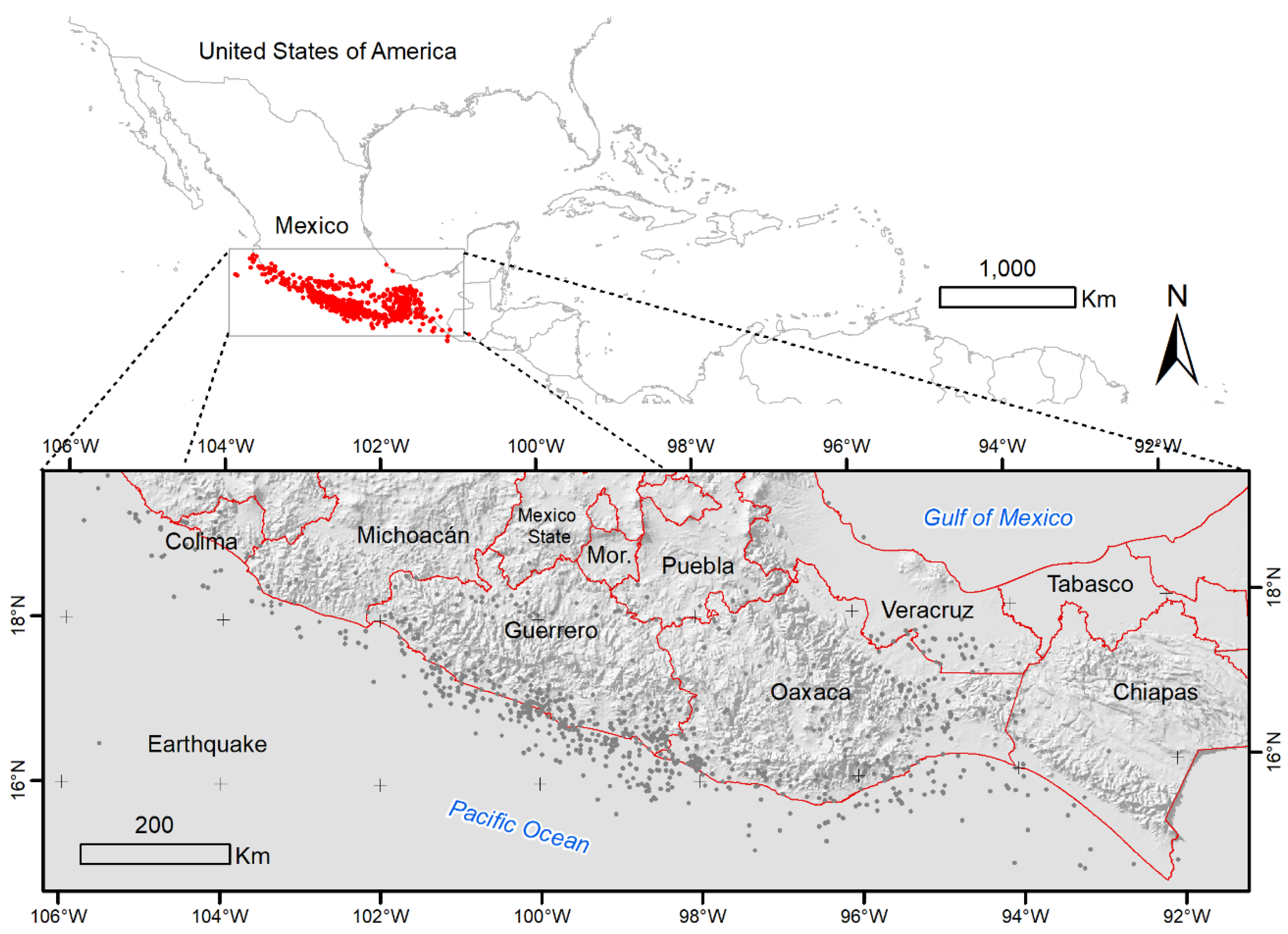
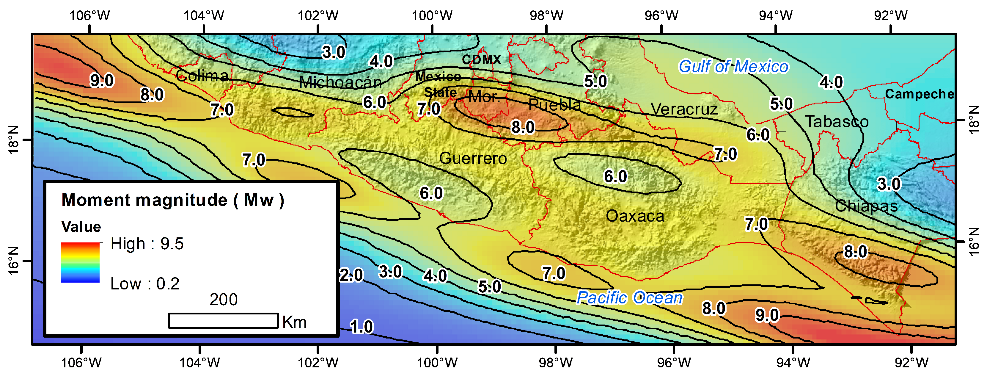
2.1. Study Area

The seismicity and tectonics of southern Mexico are characterized by the subduction of the Cocos and Rivera plates beneath the North America plate [28]. The Cocos plate has been subducting underneath the North American plate at a constant and relatively shallow angle of 12 15 at a rate of about 6 cm/year [29], affecting the seismicity of the states of Michoacan, Guerrero and Oaxaca. Similarly, the Cocos and North American plates are joined to the Caribbean plate in a trench-shaped area forming the zone of subduction of the Cocos plate beneath that of the Caribbean, increasing the seismicity in the states of Oaxaca and Chiapas. The subduction of the Rivera plate beneath the Jalisco block is relatively low, which affects the states of Colima and Jalisco. Figure 1 shows the study area as well as the spatial distribution of the maxima of earthquake intensities between 16 September 1992 and 20 February 2018.

2.2. Methodology

2.2.1. The GEV Distribution

Classical results on order statistics on the maximum of a random sample Y 1 , . . . , Y n show that the distribution of M n = m a x Y 1 , . . . , Y n degenerates its mass of probabilities into a point as the sample size increases and consequently the exact distribution of the M n is a degenerate function when the sample size is large enough. In such cases, the distribution M n can be stabilized using a sequence of constants b n > 0 and a n , through G n = ( M n - a n ) / b n . Transcendent statistical results show that the asymptotic distribution of G n is a non-degenerate, limit distribution known as the generalized extreme value (GEV) distribution [30]:
G ( y ) = exp - 1 + κ y - μ σ - 1 κ , κ 0 ; 1 + κ y - μ σ > 0 exp - exp - ( y - μ ) σ , κ = 0
where - y + , - μ + , - κ + , σ > 0 (see [31]).

2.2.2. Estimation of the Parameters of the GEV under Random Censoring

Consider a set of n independently and identically distributed random pairs ( M t , δ t ) . Specifically, in the extreme values framework, we obtain the maximum values M t , in blocks of information in which a censored value U t can exist. We assume that the variables M t and U t are independent. Let Y t = m i n ( M t , U t ) and δ t = I M t U t , a failure indicator that shows whether the value of Y t is censored δ t = 0 or not δ t = 1 . δ t is different from censoring indicator C t = I U t M t . Then, the distribution of M t , is given by:
M t G E V ( μ t , σ t , κ )
Let G t y t | μ t , σ t , κ be the probability distribution function of M t , g y t | μ t , σ t , κ is its probability density function and denote G * y t | μ t , σ t , κ = 1 - G y t | μ t , σ t , κ as its survival function. Similarly, let F u and f u be the survival and density functions of U t , respectively. The joint density function of Y t may be obtained from the joint density function of M t and U t , thus we can construct the likelihood function from a random sample of maxima as follows [16]:
L μ t , σ t , κ | y t = i = 1 n G * y t ; μ t , σ t , κ f y t 1 - δ t F y t g y t ; μ t , σ t , κ δ t
Arranging the terms, we finally obtain:
L μ t , σ t , κ | y t = i = 1 n F y t δ t f y t 1 - δ t * i = 1 n G * y t ; μ t , σ t , κ 1 - δ t g y t ; μ t , σ t , κ δ t
Assuming that the censoring is non-informative, i.e., F u and f u do not involve the parameter μ t , σ t , κ , then the likelihood on the data is:
L μ t , σ t , κ | y t i = 1 n G * y t ; μ t , σ t , κ 1 - δ t g y t ; μ t , σ t , κ δ t
We analyze the extremes on a spatial region using functions adjusted to the parameters of the GEV distribution. These functions model the trends in the maxima and relate the parameters with covariates through functions. In this research, we consider using the following linear predictors:
μ t = i = 1 P 1 X t i β 1 i + i = 1 P 2 Z t i u 1 i , l o g σ t = σ κ t = κ
where Z i j = exp - x ̲ i - k ̲ j 2 , i = 1 , , n , j = 1 , , p 2 and k ̲ j the jth centroid obtained using the method of average linkage hierarchical clustering. We construct the design matrix C joining the columns of X and Z and rewrite the linear predictors as μ t = C b 1 ; l o g σ t = σ ; κ t = κ .

2.2.3. Bayesian Implementation

The logarithmic scale in which the intensities of the earthquakes are measured directly affects the tails of the distribution of extreme values and increases the difficulty of correctly estimating the parameters. Bayesian inference helps solve this problem. Assigning an appropriate a priori distribution, we can include previous information about the parameters. We incorporate a priori information about the parameters θ t = μ t , σ t , κ of the GEV distribution, using the following hierarchical Bayesian model:
π θ t , ω | y t π y t | θ t π θ t | ω π ω
where π y t | θ t is the GEV distribution, π θ t | ω is the a priori distribution of the parameters and π ω is the a priori distribution of the hyperparameters.
Applying the conditions in the parameters given in Equation (1), we reformulate the parameter and hyperparameter sets using ω * = β 1 , β 2 , u 1 , u 2 , κ and ω * * = σ 1 , σ 2 , respectively. Therefore, the posterior distribution can be written as:
π ω * , ω * * | y t π y t | ω * π ω * | ω * * π ω * *
where π y t | ω * is the GEV density under the conditions on the parameters given in Equation (1). We regularize the model using normal distributions with zero mean for the coefficients of the linear predictor, and a uniform a priori distribution with mean −0.75 for the shape parameter. Therefore, the prior distribution set for ω * are β 1 N 0 , 10 4 I , β 2 N 0 , 10 4 I , u 1 | σ 1 N ( 0 , σ 1 2 I P 2 + D d D d ) , u 2 | σ 2 N 0 , σ 2 2 I P 2 and κ U n i f o r m ( - 0 . 9 , - 0 . 59 ) . The prior distribution for the hyperparameters ω * * is given by σ 1 2 H a l f - C a u c h y ( 25 ) and σ 2 2 H a l f - C a u c h y ( 25 ) .
We have based the parameters estimation on the average of 300,000 samples drawn by a MCMC random walk algorithm. To sample the a posteriori distribution, we generate candidates from a normal density function, and accept with probability:
α θ * | θ = m i n 1 , π x | θ * π θ * Q θ * , θ π x | θ π θ Q θ , θ *
where π θ is the prior distribution for the parameters, π x | θ is the likelihood and Q is the proposal density. Parameters obtained with the maximum a posteriori (MAP) approach are also provided. The estimators of the map method are similar to those obtained by the maximum likelihood method, which, in the case of the a priori normal distribution, bring about the regularization of the model and the shrinkage of the coefficients of the linear predictor.

2.2.4. Simulation Study

We conducted a simulation study to verify the model efficiency, the numerical convergence and the limitations in the estimation procedure. We simulated a set of 800 extremes artificially censored from a GEV model with a parametric setting given by Equation (5) and 40 percent random censorship. We chose the x 1 and x 2 covariates, corresponding to the longitude and latitude, uniformly from the interval - 91 , - 107 and 14 , 20 , respectively.
μ t = 8 e 1 2 x 1 - 17 2 + x 2 + 98 . 5 2 σ t = σ = 1 κ t = κ = - 0 . 6
To determine how the result is affected by the number of nodes in Equation (1), we adjusted two models, the first setting p 2 = 20 and the second with p 2 = 80 in Equation (1). The estimates of the shape parameter were −0.59 and −0.69, respectively. The estimates of the σ parameter were 1.38 and 1.05, respectively. The functions used to generate the trend of the maxima and defined by the scale parameter of the GEV distribution, are shown in Figure 2a. Because the function corresponding to μ involves the product of the exponentials to the square of the covariates x 1 and x 2 , it cannot be represented as the sum of additive functions of these two covariates. For simplicity, functions for the scale and shape parameter are constant.
The results of the simulation showed that the proposed model correctly estimates the actual function used for the trend (Figure 2a). Although the magnitude of the estimates differs from the original, the difference decreases as the number of knots increases, from p = 20 to p = 80 (Figure 2b,c). Similarly, a comparison of estimators of κ for both p = 20 and p = 80 reveals that estimates of the shape parameter was more accurate in the p = 20 case, with an error less than 0.01, compared with the estimate obtained with p = 80 , for which the deviation was around 0.1. In contrast, the estimators of the scale parameter are slightly skewed to the left due to the effect of the a priori distributions on the parameters.
An independent testing set of 1000 observations was simulated to validate the fitted model. The correlation between the observed and the estimates was 0.86 and 0.94 with p = 20 and p = 80 , respectively. The parameters estimated by the spline function can barely be interpreted individually because they constitute a large set of parameters, which have the main objective of approximating the nonlinear characteristics of an arbitrary function. However, because the variables have been standardized, it is possible to evaluate the effect of the change of each coefficient on the change in the parameters of the GEV distribution.

2.3. Data Collection

The data corresponded to 845 observations of monthly block maxima of earthquake intensities in the seismological scale of moments, between 16 September 1992 and 20 February 2018, obtained at 97 fixed monitoring stations of the Mexican Seismic Alert System (Figure 1). The SASMEX system is a network formed by the Sistema de Alerta Sísmica de la Ciudad de México (SAS) and the Sistema de Alerta Sísmica de Oaxaca (SASO). The SAS was designed and developed by Centro de Instrumentación y Registro Sísmico (CIRES) in 1988. A few years later, as a result of the damage caused to the state of Oaxaca by the earthquake that occurred on 15 June 1999, the state government gave CIRES the responsibility of building the SASO system. In 2012, the Oaxaca and Mexico City authorities agreed to integrate the functions of SASO and SAS into one system known as SASMEX [32].

2.4. Data Analysis

The extreme values were obtained from space-time blocks using the block maxima approach [33]. In the spatial plane, a total of 22 rectangular space blocks were generated, and the area of each block was 36,925 km 2 . In the temporal plane, the width of the time interval was one month. Thus, the rationale for censoring data in our study is as follows. Some blocks exhibited missing information (47% of the total number of blocks). Such missing observations could have values, in some cases, higher than the maximum value observed in the block (see Figure 3). However, in other cases, missing values could be lower than the minimum found, thus such observations should not be censored (unfortunately, this information is unknown), thus the maximum found value was “artificially” censored using a random threshold. Thus, the maximum value was eliminated, and the threshold estimated was assigned for the block and the observation was then flagged as “censored observation”. Furthermore, to avoid loss of information for analysis, the difference between the threshold estimated and the maximum observed was minimal. Therefore, both censored and uncensored observations data were included to estimate likelihood following the method in Section 2.2.2. We constructed a GEV model for the Maxima of earthquakes on the Pacific coast of southern Mexico, using multivariate smoothing functions of spatiotemporal covariates, latitude ( s 1 ), longitude ( s 2 ) and time (t), to fit the trends in the non stationary GEV model. To regularize the model and avoid abrupt changes between the coefficients, we assigned a N ( 0 , σ 1 2 I P 2 + D d D d ) a priori distribution to the coefficients u 1 s in the model in Equation (1), where D d (with d = 1 ) is a matrix such that D d u 1 = Δ d u 1 constructs the vector of dth differences of u 1 .

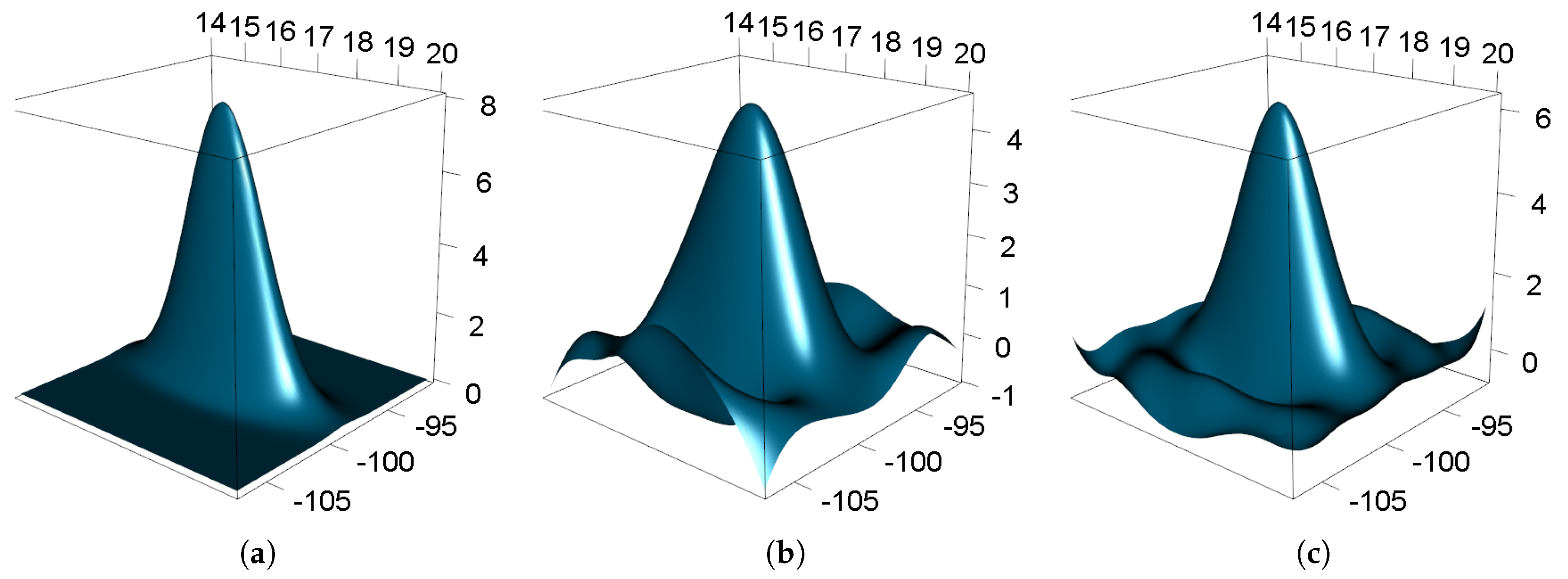
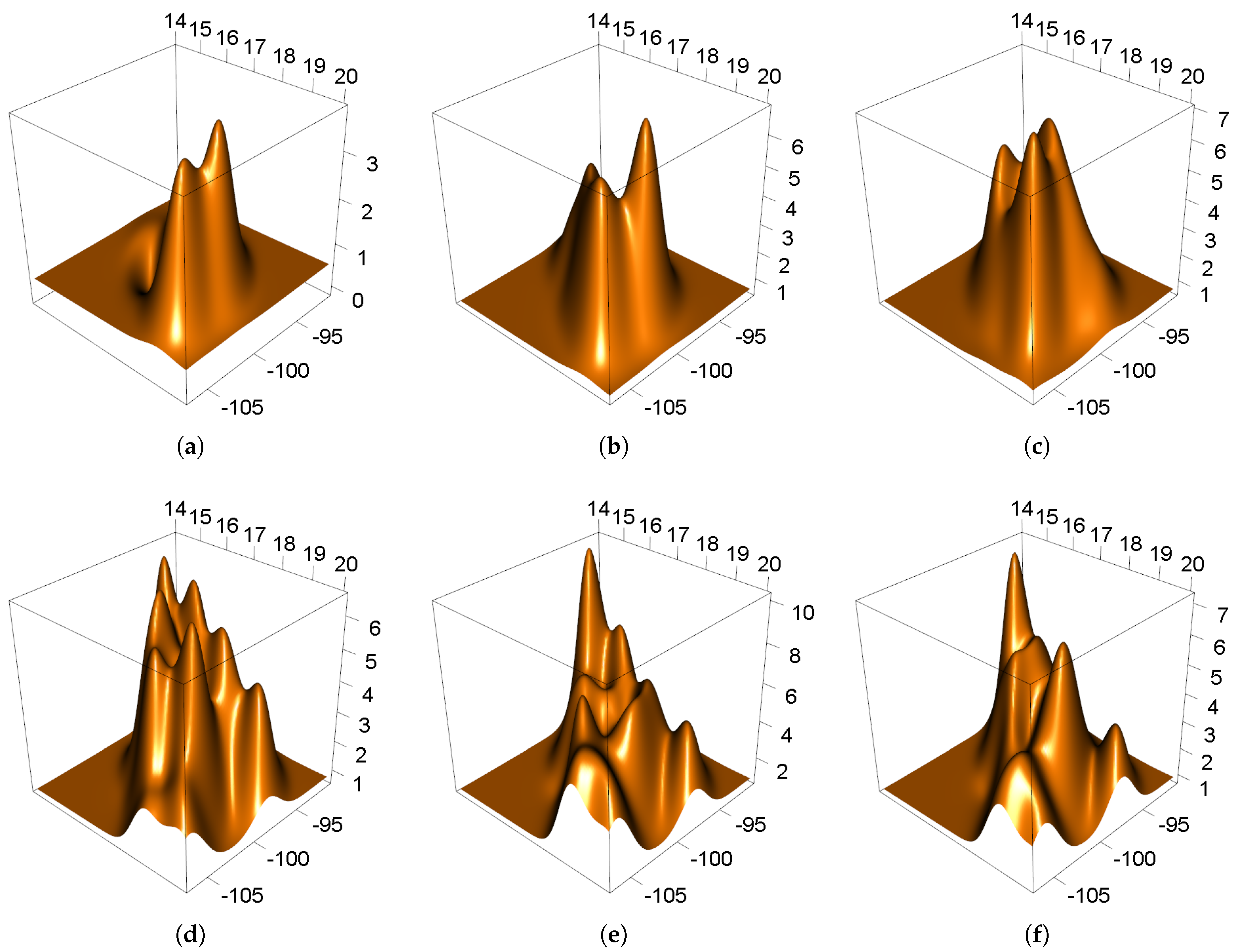
3. Results and Discussion

A descriptive summary of the data by each spatial block is shown in Table 1. In this table, we can see that the magnitude of the maxima for each block is varied and heterogeneous. In the area of Block 4, whose central point is in the parallel located at 15 N and in the meridian located at 94 . 5 W, the maximum intensity recorded was M w 8 . 2 regarding to the magnitude of the moment, in contrast to the maximum intensity measured in Block 22, where the maxima was M w 4 . 6 . In six of the twenty-two blocks, the maximum magnitude exceeded M w 7 . 0 . An important characteristic that we observed in all the blocks is that there is a marked difference between the third and fourth quartiles, which indicates that a distribution of heavy tails should be appropriate for the study of this type of data.
Clearly, tectonic and physical conditions in southern Mexico vary from region to region, causing seismic patterns that are reflected in extreme events of earthquakes in surrounding areas. Furthermore, these trends may also vary from one time period to another. We verified this behavior again in the statistics of means and quantiles presented in Table 1, which show that the magnitudes of the maxima studied tend to vary from one place to another. This fact justifies the modeling of the location parameter with respect to time and space.
The covariates used to estimate spatiotemporal trends were latitude, longitude and time. A hierarchical Bayesian model was fitted to analyze the maxima of earthquakes on the Pacific coast of southern Mexico. At the first level, we modeled the intensities of maxima earthquakes using the generalized extreme value distribution with random censorship; at the second level, we used multivariate smoothing spline functions to model nonstationary spatiotemporal extremes; and, at the third level, we assumed a priori distribution functions for the parameters of the model. Table 2 shows the estimates of the fitted model. In other words, this formulation has the advantage of analyzing maxima through hierarchical models, or stages. The first stage represents the previous information; the second stage represents the trends in the maxima; and the third stage represents the distribution of the data. We constructed the joint probabilities distribution of the parameters and the data, also known as posterior density, using the conditional distributions, mentioned above as stages, formally represented in Equation (2). The procedure used in this work can be easily replicated by: (1) constructing the likelihood function given by Section 2.2.2; and (2) running the Metropolis–Hastings algorithm with the acceptance probabilities given by Equation (4). We fitted our Bayesian hierarchical model with the conditions expressed in Equation (1), setting p 2 = 80 . The statistical analysis was performed using the R 3 . 3 . 1 software. The samples were generated using a Metropolis–Hastings algorithm, with a Gaussian random walk. We generated 300,000 samples using a burn-in period of 50,000. A look at the logarithm of the a posteriori likelihood indicates that the algorithm successfully converged.
The spatial smoothing for the years 1995, 2000, 2005, 2010, 2015 and 2018 for the location functions is shown in Figure 4a–f, respectively. Through this, we observed that the model captured the spatiotemporal patterns present in the data. Similarly, we observed variations of the location parameter in the spatial plane. Typically, these spatiotemporal variations could not be modeled using only linear functions with a few parameters, as they could not catch the complex nonlinear variations present in the seismicity phenomenon. However, it is still possible to use several types of parameterized linear functions, such as the model in Equation (1), where the interaction effects of the original covariates are included through auxiliary covariates.
Several results were obtained by analyzing the spatial smoothing set for the location parameter over time, as shown in Figure 4a–f. Firstly, we could observe that each of the functions estimated through time showed several peaks or maximums, which correspond to the places where the most intense earthquakes occur. Secondly, it can be observed that the estimated functions for the years 1995, 2000 and 2005 have similar characteristics. However, in the year 2010, the patterns began to change, until later, for the years 2015 and 2018, we observed different patterns compared to the first few years. Furthermore, the intensities of earthquakes increase over time, which shows that the risk of extreme events increases with time.
The flexibility of the proposed model allows studying the temporal variations in each geographical location on the study area. Figure 5 shows the temporal dynamics at six geographical locations in which we observed a period of increased seismic activity between the years 1998 and 2002 and a period of greater seismic activity between 2010 and 2016 that remained at high levels until the last years of the period of time studied. Consistently with these results, in 2017 and 2018, three of the strongest earthquakes of the studied period were recorded. A strong earthquake of M w 8 . 2 hit the southern coast of Mexico, on 7 September 2017, approximately 87 kilometers southwest of Pijijiapan in the state of Chiapas, being the second strongest recorded in the history of the country. Two weeks later, on 9 September 2017, a second earthquake of magnitude M w 7 . 2 , struck the states of Puebla and Morelos, in the center of the country, causing severe material and human losses. A few months later, on 16 February 2018, a strong earthquake of M w 7 . 2 hit the south coast of Mexico again, approximately 37 km northeast of Pinotepa de Don Luis in the State of Oaxaca. The probability of large earthquakes on the coasts of Oaxaca and Guerrero is greater compared to other regions, due to the proximity they have with boundary plates. However, the Puebla and Morelos earthquake hit the central zone of the country, far from the limits between tectonic plates. Recent research suggests that these earthquakes should not be unexpected. An entropy change of seismicity under time reversal, considered as a non-seismic precursor of earthquakes, was identified several months before the occurrence of the major earthquake [34,35].
In this study, we developed a model of extreme values with censoring data for the earthquakes on the Pacific coast of southern Mexico using a robust and solidly-based theory. An important application of the results of our study is through a risk map or return level map. The return level Z p is the threshold at which an extreme value is exceeded with probability p, which is expected to occur once every 1/p years [36]. Figure 6 shows the strength of earthquakes for a return period of 25 years built using a spatial model. The stability of the results shown in Figure 6 is strongly influenced by the size of the sample. Therefore, adding or eliminating a set of extreme values, the results obtained should change. The initial value of the algorithm also modifies the convergence time of the MCMC algorithm, causing in the worst case, the non-convergence of the algorithm. Isolines in the map (Figure 6) can be used to discover the spatial trend of strength of earthquakes. In fact, earthquakes greater than M w 8 regarding to the magnitude of the moment in a return period of 25 years can be expected in the Southeast part of the State of Chiapas (Figure 6). An interesting issue that explains the spatial trend of strength of earthquake is that the boundaries of the Cocos, North America and Caribbean plates are converging slightly to the south from the region that presents the highest estimated values. Further, in the boundary between Veracruz and Oaxaca States can be identified a region moderately vulnerable to the presence of earthquakes with values of strength of earthquakes higher than 7.5. Finally, a decrease of the estimated intensity of earthquakes can be detected in regions further away from the southern coast of Mexico. This research confirmed the latent risk of earthquakes in the region using empirical data gathered from a network of sensors spatially-distributed and administered by the SASMEX system. These findings should encourage using stronger specifications when building civil infrastructure in order to decrease the effect of earthquakes.
Similar to the findings reported by studies in other countries, the extreme events of earthquakes studied here exhibited spatial variations within the study area [37]. These spatial variations have also been found in the results of various types of studies on seismogenic zoning [38]. The analysis of the extreme values of earthquakes using the extreme distribution of the value in the non-stationary approach, in addition to allowing the calculation of the probabilities of extreme events, helps to solve the problem of seismogenic zoning in a limited area, by establishing suitably chosen thresholds in the isolines of the estimated smoothed function of the location parameter.

4. Conclusions

In this research work, we studied the extreme non-stationary values of earthquakes with censored data using a Bayesian approach. One of the benefits of this model is that the spline function used to calculate the parameters of the GEV distribution allows for the adjustment of a wide variety of nonlinear functions, which are common in this type of data. The parameters are estimated via Markov chain Monte-Carlo (MCMC), which has the advantage of sampling analytically intractable posterior distributions and simultaneously estimating unknown hyperparameters. It also allows the elimination of potential values of invalid parameters. Additionally, estimates were obtained by adjusting to the non-stationary GEV model, in which we corrected the likelihood function in order to consider the effect of random censorship to obtain more reliable results. Our model was validated through a rigorous simulation study that gives support and validity to our results. An important challenge is extending this work to the case when using different a priori distributions for the GEV parameters. Our findings indicate the existence of perfectly delimited areas with greater risks of occurrence of strong earthquakes. These results should help administrative authorities to improve prevention policies and standards in the case of an extreme event.

Author Contributions

Conceptualization, A.I.A.-S. and H.V.-H.; methodology, C.A.A.-S., M.G.-M. and F.B.; software, A.I.A.-S. and J.d.C.J.-H.; validation, C.A.A.-S., F.B. and M.G.-M.; formal analysis, A.I.A.-S., H.V.-H. and C.A.A.-S.; investigation, J.d.C.J.-H. and M.G.-M.; resources, F.B.; data curation, A.I.A.-S. and C.A.A.-S.; writing–original draft preparation, A.I.A.-S., H.V.-H., C.A.A.-S., J.d.C.J.-H., F.B. and M.G.-M.; writing–review and editing, A.I.A.-S.; visualization, A.I.A.-S. and C.A.A.-S.; supervision, F.B. and H.V.-H.; and project administration, A.I.A.-S., C.A.A.-S. and H.V.-H.

Funding

This research received no external funding.

Acknowledgments

The authors thank the Centro de Instrumentacion y Registro Sismico, A.C. (http://www.cires.org.mx/) for providing the earthquake data used in this research. Special thanks are also given to two anonymous reviewers who shared with us insightful observations that deeply improved our work.

Conflicts of Interest

The authors declare no conflict of interest.

Abbreviations

The following abbreviations are used in this manuscript:
EVTExtreme Value Theory
MCMCMarkov Chain Monte-Carlo
SASMEXSistema de Alerta Sísmica de Mexico
SASSistema de Alerta Sísmica de la Ciudad de Mexico
SASOSistema de Alerta Sísmica de Oaxaca
CIRESCentro de Instrumentación y Registro Sísmico

References

  1. Rundle, J.B.; Turcotte, D.L.; Shcherbakov, R.; Klein, W.; Sammis, C. Statistical physics approach to understanding the multiscale dynamics of earthquake fault systems. Rev. Geophys. 2003, 41. [Google Scholar] [CrossRef] [Green Version]
  2. Karaboga, T.; Canyilmaz, M.; Ozcan, O. Investigation of the relationship between ionospheric foF2 and earthquakes. Adv. Space Res. 2018, 61, 2022–2030. [Google Scholar] [CrossRef]
  3. Holliday, J.R.; Rundle, J.B.; Turcotte, D.L. Earthquake forecasting and verification. In Encyclopedia of Complexity and Systems Science; Springer: London, UK, 2009; pp. 2438–2449. [Google Scholar]
  4. Uyeda, S.; Kamogawa, M.; Nagao, T. Earthquakes, Electromagnetic Signals of. In Encyclopedia of Complexity and Systems Science; Springer: London, UK, 2009; pp. 2621–2635. [Google Scholar]
  5. Varotsos, P.A.; Sarlis, N.V.; Skordas, E.S. Phenomena preceding major earthquakes interconnected through a physical model. Ann. Geophys. 2019, 37, 315–324. [Google Scholar] [CrossRef] [Green Version]
  6. Sarlis, N. Statistical Significance of Earthś Electric and Magnetic Field Variations Preceding Earthquakes in Greece and Japan Revisited. Entropy 2018, 20, 561. [Google Scholar] [CrossRef]
  7. Uyeda, S.; Nagao, T.; Kamogawa, M. Short-term earthquake prediction: Current status of seismo-electromagnetics. Tectonophysics 2009, 470, 205–213. [Google Scholar] [CrossRef]
  8. Hosking, J.R.M.; Wallis, J.R.; Wood, E.F. Estimation of the Generalized Extreme-Value Distribution by the Method of Probability-Weighted Moments. Technometrics 1985, 27, 251–261. [Google Scholar] [CrossRef]
  9. Bocci, C.; Caporali, E.; Petrucci, A. Geoadditive modeling for extreme rainfall data. AStA Adv. Stat. Anal. 2013, 97, 181–193. [Google Scholar] [CrossRef]
  10. Dupuis, D.; Field, C. Large wind speeds: Modeling and outlier detection. J. Agric. Biol. Environ. Stat. 2004, 9, 105. [Google Scholar] [CrossRef]
  11. Reich, B.; Shaby, B.; Cooley, D. A Hierarchical Model for Serially-Dependent Extremes: A Study of Heat Waves in the Western US. J. Agric. Biol. Environ. Stat. 2014, 19, 119–135. [Google Scholar] [CrossRef]
  12. Nordquist, J.M. Theory of largest values applied to earthquake magnitudes. Eos Trans. Am. Geophys. Union 1945, 26, 29–31. [Google Scholar] [CrossRef]
  13. Makjanić, B. On the frequency distribution of earthquake magnitude and intensity. Bull. Seismol. Soc. Am. 1980, 70, 2253–2260. [Google Scholar]
  14. Coles, S. An Introduction to Statistical Modeling of Extreme Values; Springer: London, UK, 2001; Volume 208. [Google Scholar]
  15. Leese, M.N. Use of censored data in the estimation of Gumbel distribution parameters for annual maximum flood series. Water Resour. Res. 1973, 9, 1534–1542. [Google Scholar] [CrossRef]
  16. Kalbfleisch, J.D. The Statistical Analysis of Failure Time Data; John Wiley & Sons, Ltd.: Hoboken, NJ, USA, 2002. [Google Scholar]
  17. Einmahl, J.H.; Fils-Villetard, A.; Guillou, A. Statistics of extremes under random censoring. Bernoulli 2008, 14, 207–227. [Google Scholar] [CrossRef]
  18. Gomes, M.I.; Neves, M.M. Estimation of the extreme value index for randomly censored data. Biom. Lett. 2011, 48, 1–22. [Google Scholar]
  19. Bhattarai, K.P. Partial L-moments for the analysis of censored flood samples/Utilisation des L-moments partiels pour lánalyse d’échantillons tronqués de crues. Hydrol. Sci. J. 2004, 49. [Google Scholar] [CrossRef]
  20. Danish, M.Y.; Aslam, M. Bayesian inference for the randomly censored Weibull distribution. J. Stat. Comput. Simul. 2014, 84, 215–230. [Google Scholar] [CrossRef]
  21. Abbas, K.; Tang, Y. Estimation of Parameters for Fréchet Distribution Based on Type-II Censored Samples. Casp. J. Appl. Sci. Res. 2013, 2, 36–43. [Google Scholar]
  22. Hakamipour, N.; Rezaei, S. Optimizing the simple step stress accelerated life test with type I censored Fréchet data. REVSTAT–Stat. J. 2017, 15, 1–23. [Google Scholar]
  23. Prescott, P.; Walden, A. Maximum likeiihood estimation of the parameters of the three-parameter generalized extreme-value distribution from censored samples. J. Stat. Comput. Simul. 1983, 16, 241–250. [Google Scholar] [CrossRef]
  24. Phien, H.N.; Fang, T.S.E. Maximum likelihood estimation of the parameters and quantiles of the general extreme-value distribution from censored samples. J. Hydrol. 1989, 105, 139–155. [Google Scholar] [CrossRef]
  25. Wang, Q. Using partial probability weighted moments to fit the extreme value distributions to censored samples. Water Resour. Res. 1996, 32, 1767–1771. [Google Scholar] [CrossRef]
  26. Hosking, J.R. L-moments: analysis and estimation of distributions using linear combinations of order statistics. J. R. Stat. Soc. Ser. B (Methodol.) 1990, 52, 105–124. [Google Scholar] [CrossRef]
  27. Hosking, J.R.M. The use of L-moments in the analysis of censored data. In Recent Advances in Life-Testing and Reliability; Chapter 29; Balakrishnan, N., Ed.; CRC Press: Boca Raton, FL, USA, 1995; pp. 546–564. [Google Scholar]
  28. Pardo, M.; Suarez, G. Shape of the subducted Rivera and Cocos plates in southern Mexico: Seismic and tectonic implications. J. Geophys. Res. Solid Earth 1995, 100, 12357–12373. [Google Scholar] [CrossRef] [Green Version]
  29. Kim, Y.; Clayton, R.; Jackson, J. Geometry and seismic properties of the subducting Cocos plate in central Mexico. J. Geophys. Res. Solid Earth 2010, 115. [Google Scholar] [CrossRef] [Green Version]
  30. Jenkinson, A.F. The frequency distribution of the annual maximum (or minimum) values of meteorological elements. Q. J. R. Meteorol. Soc. 1955, 81, 158–171. [Google Scholar] [CrossRef]
  31. Fisher, R.A.; Tippett, L.H.C. Limiting forms of the frequency distribution of the largest or smallest member of a sample. Proc. Camb. Philos. Soc. 1928, 24, 180–190. [Google Scholar] [CrossRef]
  32. Espinosa-Aranda, J.; Cuellar, A.; Garcia, A.; Ibarrola, G.; Islas, R.; Maldonado, S.; Rodriguez, F. Evolution of the Mexican seismic alert system (SASMEX). Seismol. Res. Lett. 2009, 80, 694–706. [Google Scholar] [CrossRef]
  33. Gumbel, E. Statistics of Extremes; Columbia University Press: New York, NY, USA, 1958. [Google Scholar]
  34. Sarlis, N.V.; Skordas, E.S.; Varotsos, P.A.; Ramírez-Rojas, A.; Flores-Márquez, E.L. Natural time analysis: On the deadly Mexico M8. 2 earthquake on 7 September 2017. Phys. A Stat. Mech. Its Appl. 2018, 506, 625–634. [Google Scholar] [CrossRef]
  35. Stănică, D.; Stănică, D. ULF Pre-Seismic Geomagnetic Anomalous Signal Related to Mw8. 1 Offshore Chiapas Earthquake, Mexico on 8 September 2017. Entropy 2019, 21, 29. [Google Scholar] [CrossRef]
  36. Fawcett, L.; Green, A.C. Bayesian posterior predictive return levels for environmental extremes. In Stochastic Environmental Research and Risk Assessment; Springer: London, UK, 2018; pp. 1–20. [Google Scholar]
  37. Cameletti, M.; De Rubeis, V.; Ferrari, C.; Sbarra, P.; Tosi, P. An ordered probit model for seismic intensity data. Stoch. Environ. Res. Risk Assess. 2017, 31, 1593–1602. [Google Scholar] [CrossRef]
  38. Scitovski, S. A density-based clustering algorithm for earthquake zoning. Comput. Geosci. 2018, 110, 90–95. [Google Scholar] [CrossRef]
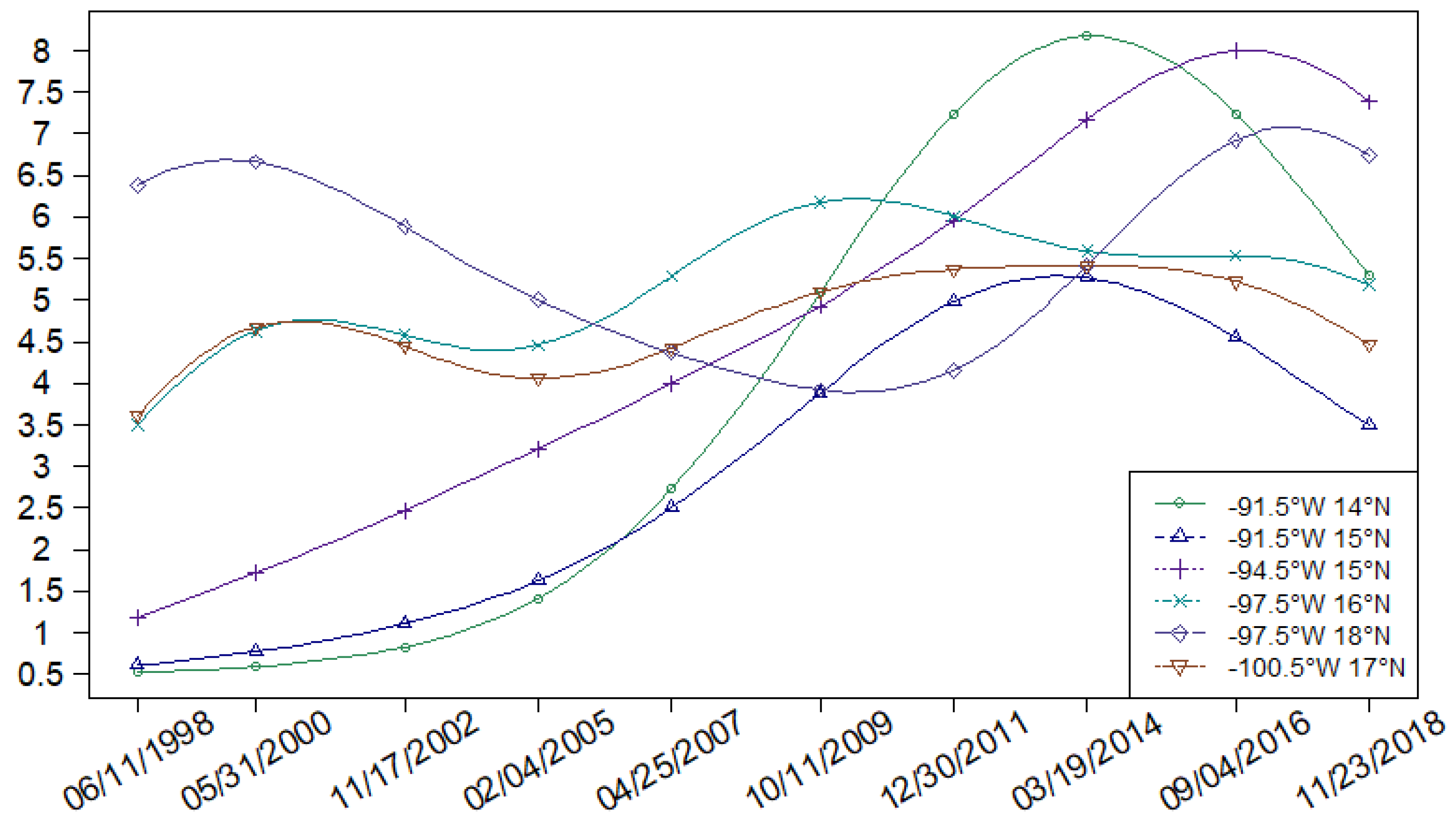
Figure 1. Study area.
Applsci 09 02863 g001
Figure 2. (a) Real functions and (b,c) functions obtained by fitting the parameters of a non-stationary GEV model with P 2 = 20 and P 2 = 80 knots, respectively, to simulated data with a sample size of n = 500 .
Applsci 09 02863 g002
Figure 3. Random censoring. X, event; M, maxima; U, censored observation. The blue dotted line shows the limits of the blocks.
Applsci 09 02863 g003
Figure 4. Estimated spatial smoothing of the location parameter for the years: (a) 1995; (b) 2000; (c) 2005; (d) 2010; (e) 2015; (f) 2018.
Applsci 09 02863 g004
Figure 5. Estimated temporal smoothing of the location parameter of earthquake maxima at six geographical locations on the Pacific coast of southern Mexico.
Applsci 09 02863 g005
Figure 6. Strength of earthquakes estimated for a 25-year return period in southern Mexico.
Applsci 09 02863 g006
Table 1. Descriptive summary information on the Maxima of earthquakes on the Pacific coast of southern Mexico.
Block IDLong  W Lat  N Min.1st Qu.MedianMean3rd Qu.Max.
1−91.5 14 6.16.26.86.77.37.3
2−91.5 15 6.96.97777
3−91.5 16 4.74.95.15.15.25.4
4−94.5 15 4.255.35.55.88.2
5−94.5 16 34.14.34.44.76.6
6−94.5 17 3.84.24.44.54.76.7
7−94.5 18 44.44.64.84.96.4
8−94.5 19 5.55.55.55.55.55.5
9−97.5 15 4.14.24.64.655.1
10−97.5 16 2.93.944.24.37.4
11−97.5 17 2.23.844.14.25.8
12−97.5 18 3.84.14.44.75.37.1
13−97.5 19 4.84.84.84.84.84.8
14−100.5 16 3.644.34.34.65.2
15−100.5 17 3.13.94.14.24.47.2
16−100.5 18 3.544.14.44.46.5
17−100.5 19 4.24.34.44.34.44.4
18−103.5 17 5.15.15.15.15.15.1
19−103.5 18 3.744.34.54.76.5
20−103.5 19 3.744.14.34.45.9
21−106.5 19 4.14.24.24.85.36.3
22−106.5 20 3.844.14.24.34.6
Table 2. Estimates and 95% credible intervals of the non-stationary GEV model for the maxima of earthquakes.
Coef.ModeMean95% CI
β ( 1 ) 0 0.81360.7004(0.4677, 0.8079)
σ 0.57101.1110(1.0855, 1.1697)
κ −0.5900−0.5930(−0.6014, −0.5900)
σ 1 2 26.136383.3487(26.2751, 810.0938)

