The Rapid Establishment of Large Wind Fields via an Inverse Process

Abstract

Physical-approach-based wind forecasts have the merit of a heavily reduced uncertainty in predictions, but very often suffer from a prohibitively lengthy numerical computation time, if high spatial resolutions are required. To tackle this hurdle, proper orthogonal decomposition (POD) has manifested extraordinary power in reducing the number of computation grids and hence the computation time. However, POD itself suffers from difficulties in extracting basis vectors when the snapshots contain large amounts of data, when considering large areas using high spatial resolution. By means of computational simulations and inverse process analyses, in this study the authors developed a new method for rapid wind field reconstruction with high spatial resolution, while reducing the computation load to a minimum. The strategy is to establish snapshots of velocity fields in a large area, but only using a much smaller subset of the large area to extract the basis vectors. The basis vectors are then used to reconstruct the wind field of the large area with a high spatial resolution. The method can dramatically reduce the overall computation work due to the much smaller grid size in the subset area. The new method can be applied to situations where the velocity distributions for a large area need to be known with high spatial resolution.

1. Introduction

Wind power is one of the most rapidly growing renewable energies and is regarded as an appealing alternative to conventional power generated from fossil fuel. However, due to the intermittency of wind speed, large-scale wind power penetration will affect the quality of an electric grid, which makes the safe and stable operation of an electric power system a great challenge. In order to reduce the impact of large-scale wind power integration, accurate and effective wind power prediction is necessary to improve the limitations of wind power penetration [1]. As the wind power mainly depends on wind speed, most wind power prediction models will at first forecast wind speed and then convert wind speed to wind power according to certain power curves.

Over the years, many methods have emerged that utilize statistical processing via local or numerical wind prediction (NWP) data for wind speed forecasts. For example, a hybrid methodology based on support vector regression is proposed for wind forecasting in [2], which shows more accurate results than those from NWP. Wind field accuracy can also be substantially improved by using the Kalman filter as a post-processing procedure [3]. With the advance of modern intelligent algorithms, statistical forecast methods have been growing strongly, as they have the advantage of suiting different topographical and historical data. However, since the majority of statistical prediction models are essentially based on local historical data, these methods may intrinsically be prone to significant uncertainty in predicting future conditions. It is desirable to establish models that can provide more assurance for forecasting.

In contrast to statistical methods, physical approaches apply mechanical and thermal principles and numerical methods, such as computational fluid dynamics (CFD), to produce wind speed forecasts. Forecast methods based on physical approaches can usually provide wind speed and its associated parameters such as pressure, humidity, and temperature. Their upscaling algorithm can be based on the correlation between the representative wind farm power generation and the total power data over a certain period of measurements. There are several studies about upscaling algorithms. For example, in [4] it is proven that rough set theory is a useful tool for short-term multistep wind power prediction when combined with multiposition NWP data. A downscaled simulation framework can also be applied to carry out a multi-scale simulation of time-varying wind fields [5]. However, the calculation capacity of physical models is restricted by the complexity of its conditions as indicated by earlier studies [6], as the high number of computational grid points requires enormous computational resources and time. Therefore, any physical method will be welcome if it can yield rapid predictions based on meteorological data or real time data from other sources.

Recently, a new methodology for reconstruction that employs CFD generated data and a limited number of real time measurements at distributed locations has emerged. In this methodology, CFD is used to calculate the distribution of a data set in the field so that the data set can be obtained before the prediction, which facilitates the process of reconstruction. Proper orthogonal decomposition (POD) is then used to capture dominant features of the data set and subsequent POD modes can be used to reconstruct the whole field. This methodology can meet the requirements of real-time field prediction in many situations such as underwater acoustics [7] and aerodynamic design [8].

In our previous study, we applied this method to the reconstruction of wind fields and obtained comparatively satisfactory results [9]. This method, which very often involves an inverse process, can drastically reduce the quantity of the computational work, e.g., by three or four orders of magnitude, and reconstruct velocity fields at a very fast speed, which effectively enables onsite short-term wind forecasts.

However, the POD method still needs a large number of samples of the velocity fields, i.e., “snapshots,” to extract the basis vectors of very small matrix dimensions. Although the POD method enables the fast reconstruction of wind fields by using small matrix dimension basis vectors, the extraction of the basis vectors itself will cost immense computational work when the snapshots correspond to large areas and the spatial resolution for these areas is high.

In view of the above discussion, it is therefore the purpose of this study to establish a new approach to tackle the problems facing the POD method. This new approach will be a physical approach based on CFD simulations to minimize the uncertainty of the forecasts in the wind field. More importantly, the new approach aims to help the POD procedure extract its basis vectors, even for very large areas with high spatial resolutions, so that it can be applied to large-area wind field reconstructions.

2. Methods

2.1. Trodational POD and Gappy POD

POD (proper orthogonal decomposition) is an effective way to reduce the data dimensions and rapidly reconstruct a large area. It already has many successful applications in data processing such as the derivation of the dynamic mode [10] and the stability analysis and the design of airfoil profiles [11]. POD satisfies the requirement of a low computing cost while in many circumstances having acceptable accuracies, which may be an effective tool to rapidly reconstruct a wind field with acceptable accuracy, where a large amount of data is processed [12].

POD uses “snapshots” to extract its basis vectors. The snapshots of the POD method can be obtained from either experimental measurements or from numerical simulations. The POD snapshots in this paper come from CFD simulations. For a given area, a CFD calculation is performed to generate the velocity distributions. A series of snapshots of the velocity distributions are then collected and denoted as $U^{\mathit{l}}$, where the superscript $l$ indicates the $lth$ snapshot.

Consider the collection of m snapshots, ${\left\{U^{\mathit{l}}\right\}}_{l=1}^m$. The correlation matrix $R$ is formed by computing the inner product for every pair of snapshots.

$$R_{\mathit{i}\mathit{k}}=\frac{1}{m}\left(U^{\mathit{i}},U^k\right)$$

(1)

where $\left(U^{\mathit{i}},U^k\right)$ denotes the inner product of $U^{\mathit{i}}$ and $U^k$. The eigenvalues ${\lambda }_i$ and eigenvectors ${\mathsf{\psi }}^{\mathit{i}}$ of $R$ are computed by singular value decomposition (SVD). The $jth$POD basis vector ${\mathsf{\Phi }}^j$ is given by a linear combination of snapshots.

$${\mathsf{\Phi }}^j={\displaystyle \sum }_{i=1}^m{\mathsf{\psi }}^{\mathit{i}}{U}^{\mathit{i}}$$

(2)

where ${\mathsf{\psi }}_i^j$ denotes the $ith$element of the $jth$eigenvector. The magnitude of the $jth$ eigenvalue describes the relative importance of the $jth$ POD basis vector. For each basis vector, the importance is quantified by defining the relative energy $E_j$, which means the percentage of the $jth$ eigenvalue in the sum of the whole eigenvalues.

The POD method can also be employed to reconstruct the missing or gappy data from the partial measurement data. To do this, the first step is to define a mask vector that describes a particular field vector to identify where the data are available and where the data are missing.

For the solution $U^k$, the corresponding mask vector $n_i^k$ is defined as $n_i^k=0$ if $U_i^k$ is missing; $n_i^k=1$ if $U_i^k$ is known, where $U_i^k$ denotes the $ith$ element of the vector $U^k$; the dot product is defined as ${\left(n^k,U^k\right)}_i=n_i^k{U}_i^k$; the induced norm is defined as ${\left({\Vert v\Vert }_n\right)}^2={\left(v,v\right)}_n.g$ is set to be a solution vector that has some missing elements and is associated with the mask vector $n$, so the repaired vector $\tilde{g}$, i.e., $g$, with all the missing data “recovered,” can be approximated by

$$\tilde{g}={\displaystyle \sum }_{i=1}^p{b}_i{\mathsf{\Phi }}^{\mathit{i}}.$$

(3)

The coefficients $b_i$ in the POD method can be acquired by solving the following minimization function:

$$Error=\Vert g-\tilde{g}{\Vert }^2=\Vert g-{\displaystyle \sum }_{i=1}^p{b}_i{\mathsf{\Phi }}^{\mathit{i}}{\Vert }^2$$

(4)

where $\Vert ·\Vert$ defines the L-2 norm. It is worth mentioning that in Equation (4) only the elements with existing data in $g$ are compared with $\tilde{g}$.

In order to obtain the solution for the minimum error, one can let the partial derivative with respect to $b_i$ equal to zero. Therefore, matrix $M$ can be obtained by a series of calculations:

$$M·B=F$$

(5)

where $M_{ij}=\left({\mathsf{\Phi }}^i,{\mathsf{\Phi }}^j\right)$, $F_i=\left(g,{\mathsf{\Phi }}^i\right)$, and $B$ contains the solution vectors of $b_i$. The specific mathematical derivation process of POD can be referred to [13].

2.2. The New Algorithm

To realize the POD method for a physical-approach-based wind forecast, samples, or snapshots, of the wind velocities will be calculated using certain numerical methods—very often CFD.

A problem pertaining to this POD procedure tends to occur during the extraction of the basis vectors $\mathsf{\Phi }$ when the snapshots $U^{\mathit{l}}$ contain large amounts of data, resulting in unbearably high demands on computing resources and time. This problem will inevitably happen if the number of computational grid points is very high, as it is the result of the large computation domain and fine grids/high-spatial resolution. This problem will be more pronounced in the cases of short-term wind forecasts because time is crucial for such forecasts.

To solve the problem of extracting the basis vectors of the POD matrix, a subset of the wind field is defined in the procedure. This approach is based on the capability of the gappy POD method in recovering missing data during the reconstruction process, with the consideration that the missing data are outside the original domain. The new algorithm is formed by the following sequence:

• A series of velocity distribution profiles for a large area is generated by offsite CFD simulations ${\left\{U^{\mathit{l}}\right\}}_{l=1}^m$.
• A sub-domain ${\left\{U^{\mathit{l}}\right\}}_{l=p}^q$, i.e., a small area such as a wind farm within the large area, is selected, and a group of snapshots of wind velocities over this subset of the large area is obtained. A group of basis vectors $\mathsf{\Phi }$ of the snapshots ${\left\{U^{\mathit{l}}\right\}}_{l=p}^q$ is extracted from the subset domain by Equation (2).
• Wind speed is measured at a small number of selected locations as the real time input for the wind field reconstruction in the next step.
• The wind velocity profile for the larger area is reconstructed with a refined mesh via gappy data reconstruction methods, using Equation (3) with the limited amount of real time data from the above step.

The first and second steps of the above algorithm can be performed offsite, as wind forecasting is not involved. Therefore, the time consumption is not a concern, since no real time data are needed during these steps. The wind forecast is made in the third step. In the third step, only a single step matrix calculation is needed to obtain the velocity distribution. One of the essences of this method is that the dimension of the matrix can be several orders of magnitude lower than those used in the CFD calculations. This allows the wind velocity to be reconstructed very quickly, virtually in real time.

In addition, there is no restriction in selecting the subset of the full area. The choice can be very flexible or specified by the operators of the windfarm. For example, if a wind forecast is to be made, the subset domain can be chosen at the wind farm itself. One way of doing so is to calculate the wind velocity distribution for the large area and then draw the velocity profile at the mesh points within this subset domain. This is, however, at this moment an intuition, and its performance will be examined in the following sections.

3. Simulations

3.1. Step One: Velocity Distribution Generation for the Large Area & Step Two: Selecting a Sub-Domain and Extracting POD Basis Vectors

Wind velocity snapshots were generated. To generate the snapshots of the velocity distribution by CFD, a cuboidal computation domain was set up with a ratio of the dimensions of 1:3:5, i.e., height/width/length. Inside the domain, several models imitating small hills were arranged to generate a number of flow patterns, as shown in Figure 1 and

Table 1. The size and coordinate of the four models.

Models	Coordinate(m)
	Radius	X	Y	Z
Half-ellipsoid	0.3/0.2/0.15	0	2	0
Hemispheroid1&2	0.15	±0.3	2.3	0
Hemispheroid3&4	0.15	±1	4	0
Hemispheroid5&6	0.15	±1	1	0

.

As a prerequisite for POD, CFD was used to generate a large amount of velocity data for a simulated wind field. For a steady state flow condition and ignoring temperature variations, the conservation equations used were

Continuity equation:

$$\frac{\partial \left(\rho u\right)}{\partial x}+\frac{\partial \left(\rho v\right)}{\partial y}+\frac{\partial \left(\rho w\right)}{\partial z}=0.$$

(6)

Momentum equations:

$$\{\begin{array}{c}\frac{\partial \left(\rho u^2\right)}{\partial x}+\frac{\partial \left(\rho uv\right)}{\partial y}+\frac{\partial \left(\rho uw\right)}{\partial z}=-\frac{\partial p}{\partial x}+\frac{1}{R{e}_r}\left(\frac{\partial {\tau }_{xx}}{\partial x}+\frac{\partial {\tau }_{xy}}{\partial y}+\frac{\partial {\tau }_{xz}}{\partial z}\right)\\ \frac{\partial \left(\rho uv\right)}{\partial x}+\frac{\partial \left(\rho v^2\right)}{\partial y}+\frac{\partial \left(\rho vw\right)}{\partial z}=-\frac{\partial p}{\partial y}+\frac{1}{R{e}_r}\left(\frac{\partial {\tau }_{xy}}{\partial x}+\frac{\partial {\tau }_{yy}}{\partial y}+\frac{\partial {\tau }_{yz}}{\partial z}\right)\\ \frac{\partial \left(\rho uw\right)}{\partial x}+\frac{\partial \left(\rho vw\right)}{\partial y}+\frac{\partial \left(\rho w^2\right)}{\partial z}=-\frac{\partial p}{\partial z}+\frac{1}{R{e}_r}\left(\frac{\partial {\tau }_{xz}}{\partial x}+\frac{\partial {\tau }_{yz}}{\partial y}+\frac{\partial {\tau }_{zz}}{\partial z}\right)\end{array}$$

(7)

where u, v, and w are the wind velocities in x, y, and z coordinates, respectively, p is pressure, ρ is the fluid density, μ is the fluid dynamic viscosity, τ is the stress tensor, and Re is the Reynolds number.

Commercial software COMSOL Multiphysics was used for CFD simulations. For the boundary conditions, the outlet was set to “pressure-outlet,” and the inlet boundary condition was set to “velocity-inlet.” The SST k-ε turbulence model was used with the second-order upwind difference scheme. Standard wall functions and model constants were set to the default values in the software. The initial pressure was set to 1 bar. The solution method was “SIMPLE”; the Gradient was set to “Least Squares Cell Based,” and the Pressure was set to “Second Order,” with Momentum and Turbulent Kinetic Energy using the “Second Order Upwind” scheme. The convergence residual was set to less than 10⁻⁶. Adaptive unstructured tetrahedral meshes were used that have given a satisfactory performance.

In this simulation, the resulting number of mesh elements was 147,500 and is shown in Figure 2. CFD calculations were carried out for a series of inlet wind velocities and directions: 6, 12, and 15 m/s, each associated with an entrance angle of 0°, 30°, 60°, 90°, 120°, and 150°, respectively. Figure 3 shows a representative wind velocity distribution in the large area, corresponding to an inlet velocity of 10 m/s. It can be seen that in the open space the wind velocities remained largely consistent with the inlet velocity, i.e., about 10 m/s, while the velocities immediately before the models became slightly lower, owing to the blocking effect caused by the object. The velocities behind the object seemed also slightly lower, which is consistent with the principles of fluid mechanics.

A sub-domain was selected as indicated by the square in the lower middle part inside the large area, as shown in Figure 4. The number of mesh points within this sub-domain was 1270. The sub-domain was centered at (0,2).

3.2. Step Three: Collecting Measurement Data on a Coarse Mesh

With the POD basis vectors ready, it is possible to use the onsite measurements to reconstruct the wind velocity distributions in virtually real time. For this, the wind velocity at some sampling points needs to be taken from a certain number of onsite sensors. Since for a real time forecast it is not possible to deal with a large quantity of mesh points, which would be very time-costly to process, data from the sensors must be from a much coarser grid. For this, a coarse grid was set up containing only 2300 mesh points as shown in Figure 5.

For the measurement data generation for later comparison, CFD simulations were carried out under the same boundary conditions as those for the fine mesh case. The number of mesh points in the domain was 2300. The bottom edge was the inlet boundary. A typical result is shown in Figure 6, which corresponds to an inlet wind velocity of 10 m/s. This velocity map agrees very well with the map on the fine mesh, i.e., Figure 3.

Data were taken from this coarse wind speed map as the input data for the POD reconstruction of the wind velocity distribution in the 147,500-mesh-point network.

3.3. Step Four: Reconstruction of the Wind Velocity for the Large Area on the Fine Mesh Network

As the input data for reconstruction of the real time wind velocity distribution, 20 data points were collected from the above coarse mesh wind speed map, as the measured data. Equation (4) was then used to reconstruct the velocity map. The reconstructed velocity map is shown in Figure 7.

As only 20 measured data points were used as the input, the reconstruction was very fast, virtually within a time scale of 10 s. For error assessment, the reconstructed velocity map, namely Figure 7, was compared with the map generated by CFD with the fine mesh, i.e., Figure 3. The error map is shown in Figure 8.

From Figure 8, it can be seen very clearly that everywhere in the large area the errors are very small. In most places, the errors are below 1%, and the largest errors are below 3%. This shows that the new method works very well for wind forecasts in large areas.

4. Experiment

According to the reconstruction method and the simulation results, we used our existing test platform to perform the verification test with an equal scale reduction of simulation.

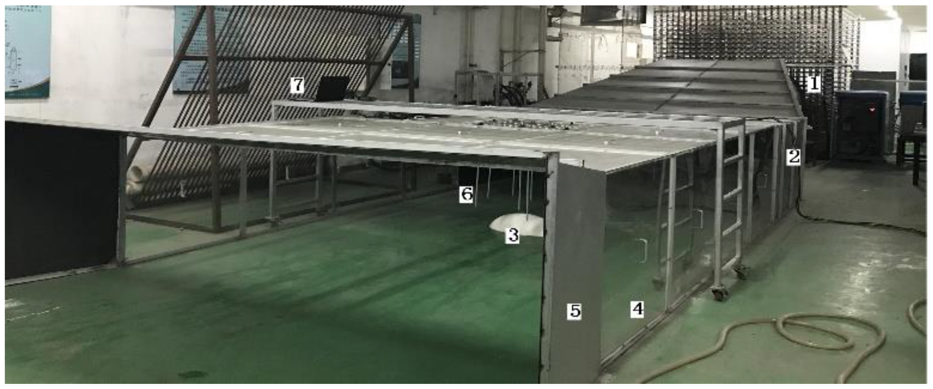
The wind tunnel, which was 10 m in length, was built and made up of a mixed-up air blower and a contraction segment, which was used to adapt to the downstream experimental section, and final diffuser section. The central experimental section had a 3 × 5 × 1 m cuboid area, which was constructed with Plexiglas plates. Models were put in the experimental section, and hot-wire anemometers were installed on top of Plexiglas surrounding the models. The experiment facilities are shown is Figure 9.

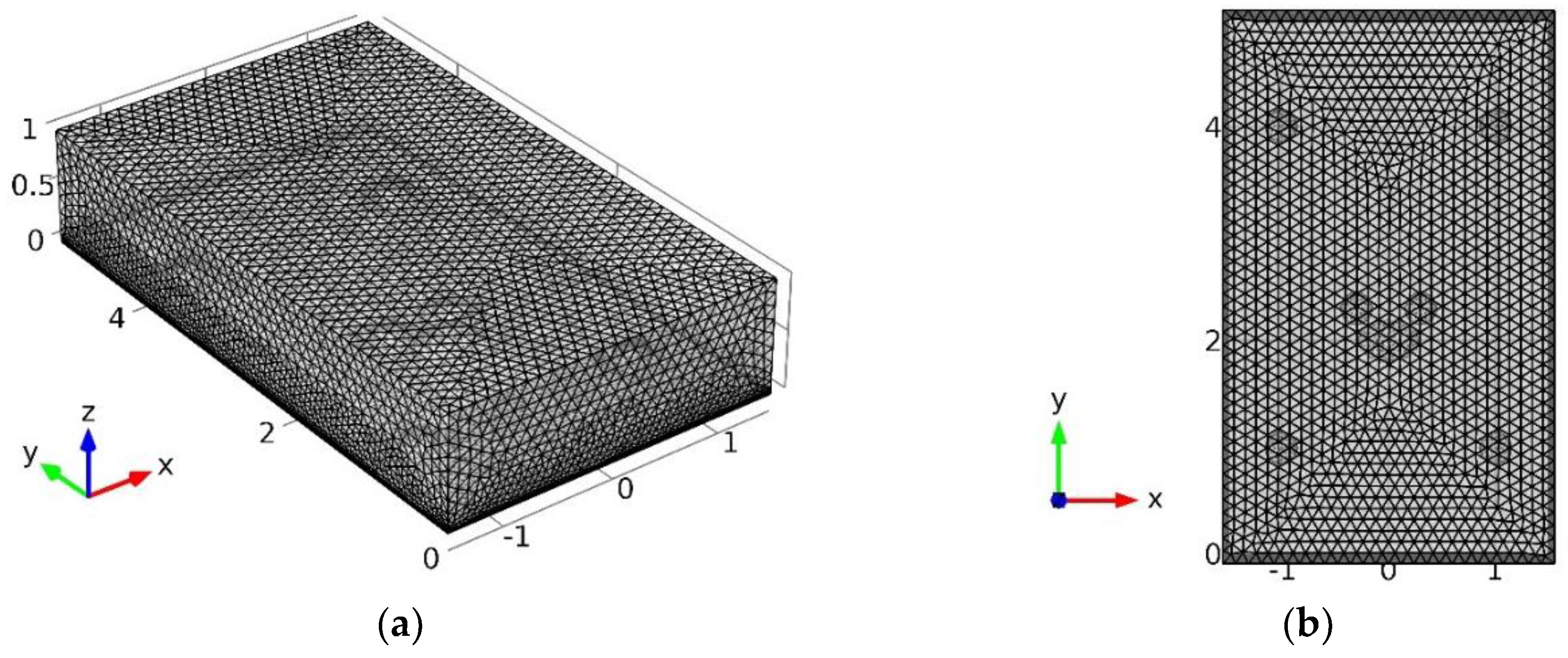
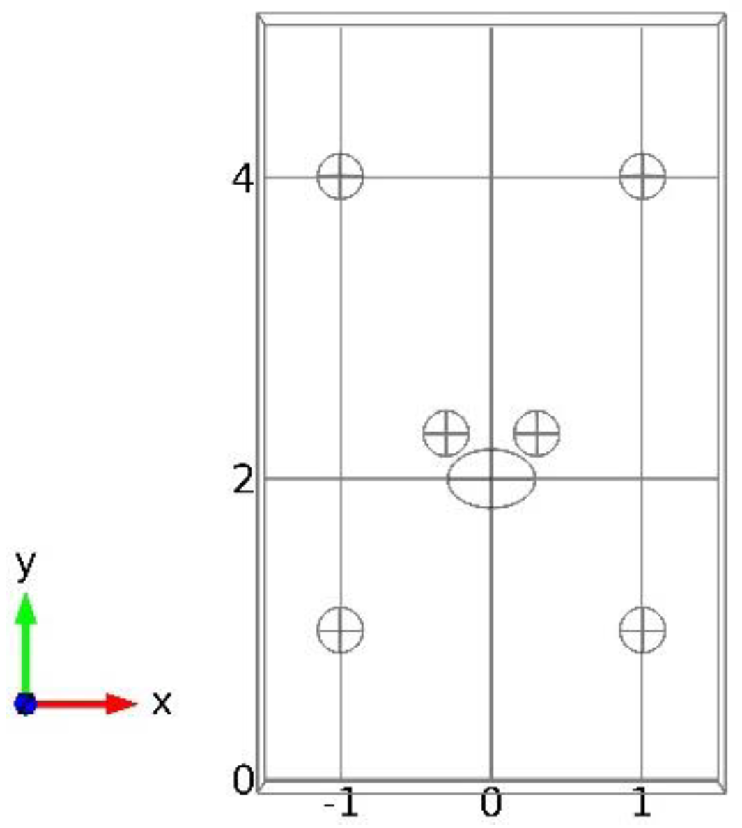
According to simulation, we conducted the experiment at a 2D level and selected the meshed experimental plane to be 20 cm away from the ground, as shown in Figure 10. A subset of the whole space of $1\times 1\mathrm{m}$ was meshed with a size of $10\times 10\mathrm{cm}$, while another area was meshed with a size of $25\times 25\mathrm{cm}$.

First, offset CFD simulations were done in a sub-domain of $1\times 1\mathrm{m}$ by refined meshes, and a group of basis vectors was extracted. Since the test bed was scaled down by simulation, the specific software settings are the same as in Section 3.

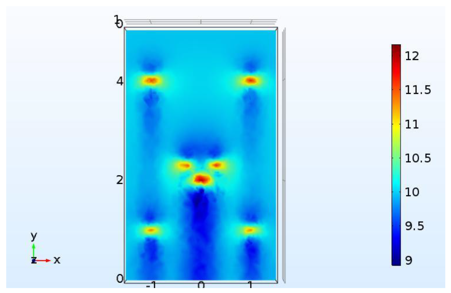
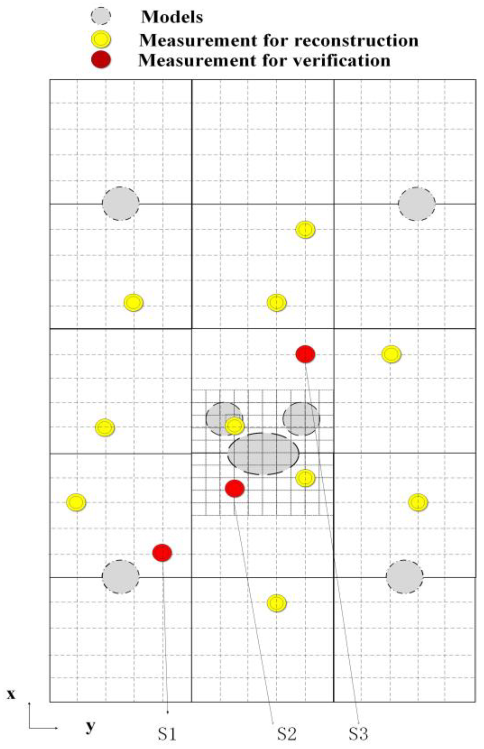
Online measurements were made in the whole plane in the coarse grid points when the inlet velocity was set to 6 m/s. Ten sensors were installed randomly in the coarse grid points, as shown by the yellow dots in Figure 10. The whole wind field can be reconstructed via gappy data reconstruction methods.

Three extra sensors were installed as a validation group to verify the results of reconstruction. One control group was set: data were reconstructed by POD basis vectors at these points. The other group consisted of data by CFD simulation with the coarse meshes when the inlet velocity was set to 6 m/s. The results are shown in

Table 2. The error comparison between measurement data and reconstructed data.

Point	Senor Measurement (m/s)	Reconstructed Data (m/s)	Relative Error (%)
S1	5.840	6.103	4.311
S2	6.052	6.276	3.573
S3	5.524	5.810	4.922

. The relative error represents the error between the sensor measurement and the reconstructed data.

It can be seen visually in Table 2 that all errors of the three points is less than 5%. Since sensors also exhibit some measurement error, 5% is an acceptable result. In addition, three validation points were selected, respectively, at locations far away from the sub-domain, in the sub-domain, and near the sub-domain, and the reconstruction errors were similar. We can conclude that the method we put forward can correctly reconstruct wind field.

5. Conclusions

An efficient wind field reconstruction method was studied that combines the POD method and the CFD method. As a new approach, a subset of the large area was defined to extract basis vectors for POD reconstruction. The new approach allows the POD method to be applied to reconstruct a wind field for large areas with high spatial resolutions. The simulation and experiments showed good results, as we expected.

Compared with previous methods, this method reduces the amount of offline work. POD basis vectors are only obtained by CFD simulation in the sub-domain area. In addition, measurements can be obtained by sensors in coarse meshes in large areas. Both the simulation and experiments showed good results.

This new approach can find applications with respect to problems of a similar nature, such as compressed sensing and process tomography.