1. Introduction
Real-time measurements are important to research studies characterizing short-term variability such as measuring rapidly changing source emissions, quantifying the amount of black carbon (BC) including short-lived pollutants emitted by mobile sources such as vehicles, or monitoring dynamic trends in indoor or ambient air quality [
1]. Previously, instruments emerged from either technology-intensive private companies or research laboratories and was used first by a small number of high-skill early adopters [
2]. The usage and development process of microAeth
® AE51 (AethLabs, San Francisco, CA, USA), however, seem slightly different from that of most other analytical devices. Many of microAeth
® AE51 have been used for exposure measurements because of their easy handling features similar to other personal air quality sensors and deployed to measure ambient BC as well. A wide range of researchers, including university labs, private companies, and government scientific research teams have used personal air quality sensors, though there has been a demand that addresses issues around interferences, humidity, calibration, and data usability [
2]. Measurement devices are upgraded through the feedback from various users who have tested them in the field and have reported their characteristics, which is a development process as well in a broad sense.
Incomplete-combustion-generated BC absorbs solar radiation and influences aerosol radiative forcing by directly changing the single scattering albedo (SSA) and by altering the lifetime of a cloud droplet, so called, through “semi-direct” effects [
3,
4]. Not only the climate effects, but health effects have also been addressed with respect to BC, because BC may cause cancer. BC concentrations have been measured by filter-based absorption instruments such as the aethalometer, the particle soot absorption photometer, the multi-angle absorption photometer, and the tri-color absorption photometer due to their ease of operation [
3,
5,
6,
7]. The aethalometer measures BC by detecting the difference in attenuation by particles collected on a filter at a given sampling interval. The particle soot absorption photometer adopts the same principle as the aethalometer but uses a different wavelength of light source. The multiangle absorption photometer measures backward scattering at two different positions to correct attenuation by the backward scattering. The tri-color absorption photometer detects attenuation at three different wavelengths with a similar principle to the aethalometer. Some instruments among mentioned above display the equivalent black carbon (eBC) mass concentration others report the light absorption coefficients. It is straightforward to measure BC under high concentration condition. However, it is challenging to measure BC concentration where the BC concentration at the region of interest becomes close to the detection limit of the instrument. In this case, taking a running-average improves the data quality produced by the instrument. The running-average, however, is a simple mathematical calculation to analyze data without having a particular meaning for black carbon. An alternative method to reduce noise in aethalometers has been proposed by Hagler et al. [
1] in the name of an optimized noise-reduction averaging (ONA) though it is currently no longer updated for newer operating systems. The principle regarding “attenuation” (ATN) is simple, but converting the ATN into BC concentration is complicated, because both scattering and absorption are involved in the attenuation.
A well-known issue in BC measurement by aethalometer-type instruments is the sensitivity. Filter-based optical techniques always suffer from the sensitivity issue. This sensitivity is directly related to the loading rate of particles on the filter materials, the air flow rate, and the sample spot size [
1]. The presence of instrumental noise regarding optics and electronics can lead to ATN values remaining unchanged or even slightly decreased when sampling at 1 s or in very low BC concentration environments, while ATN should always be increasing [
1]. Thus, corrections for scattering, filer loading, sampling spot size variation, and decrease in ATN are encouraged. Even though corrections are required, many studies associated with mobile monitoring of BC and personal exposure studies often report no correction for filter loading of the microAeth
® AE51 [
8,
9,
10,
11,
12,
13,
14,
15,
16].
The purpose of this study, however, is not to develop a new correction algorithm or procedure but to show the potential users of aethalometer-type instruments the state of the instruments as it is. There is anecdotal information that noise is amplified when the microAeth® AE51 is plugged to an AC-DC converting adaptor. This noise amplification has been known in the community though not confirmed in academic literature. The author has struggled to find examples in the peer-reviewed literature where researchers have presented a noise issue through monitoring, and this seems unusual when compared with other aethalometer-type instruments. Whilst academic usage has been modest, public uptake of BC sensors has a potential to grow. Motivated by the above discussion, we aim to investigate the errors regarding microAeth® AE51 by assessing its ability to reduce bias caused by the alteration of power source during a measurement.
2. Experimental Methods
Two microAeth® AE51s were simultaneously tested at indoor environment to eliminate temperature and humidity issues because the indoor office where this test was conducted controlled the temperature and humidity at certain values during day and night. For this reason, no correction for devices was required to display the data. One microAeth® AE51 produced in 2014 is denoted by Inst_1 and the other one, purchased in 2012, is denoted by Inst_2. New filter stripes were installed inside both devices before starting comparison test in order to minimize the overloading effect by the filters on the attenuation. The clocks of two devices were synchronized before starting measurement in order to compare data minute by minute based on the standard time. The sampling flow rate was set to 0.1 L/min (lpm) for stable collection of data.
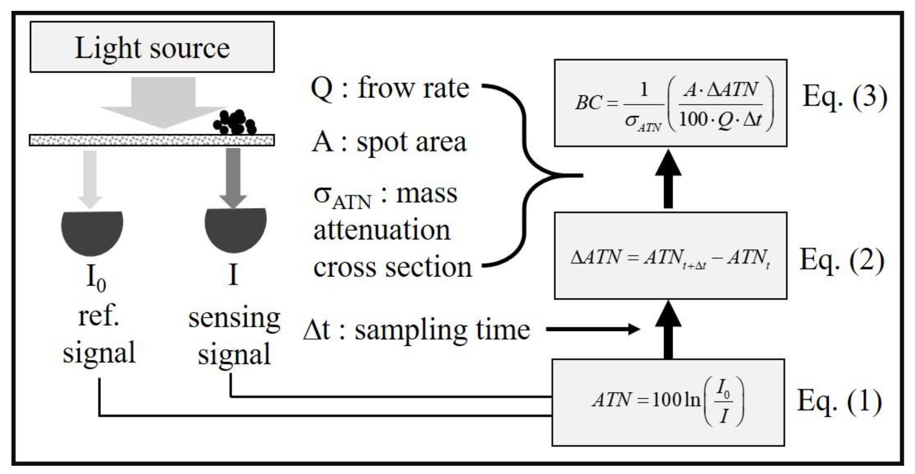
It is well known that the
ATN is defined as below based on the Beer-Lambert law.
In Equation (1), the number 100 was added for convenience.
I0 is the intensity of light transmitted through a reference blank spot, and
I is that through the spot of aerosol deposited on filter. The measurement of
I0 and
I at time
t produces
ATN at time
t, which is denoted by
ATNt. The measurement at the next time step (
t + ∆
t) produces
ATNt+∆t. Then, the changes in
ATN during the time interval (∆
t) is calculated as shown below in Equation (2).
According to Hansen et al. [
5], the
ATN is used to estimate BC concentration using the following equation.
In Equation (3), σ
ATN is the mass attenuation cross section,
A is the spot area on filter, and
Q is the sampling flow rate. The mass attenuation cross section used for microAeth
® AE51 is known to be 12.5 m
2/g [
17,
18]. The spot area is assumed to be constant unless there is a leak. The spot area is reported to be 7.07 mm
2 [
18]. The sampling flow rate in the current study is set to 0.1 lpm. The time interval is 60 s.
Figure 1 summarizes the procedure of calculating BC concentration from the real-time signals.
Uncertainty propagation analysis is performed for the BC concentrations to better understand how many errors are associated with each elements of measurement variables. Combining Equations (1)–(3) produces the following Equation.
Error propagation can be calculated from Equation (4) as below. See Appendix for more detail.
In Equation (5) the last term ensues from the sensitivity of detectors. It may be estimated from Equation (5) how sensitive sensors are required in order to satisfy a given uncertainty of the BC concentration. Backman et al. [
7] addressed the fact that the uncertainty in BC has more than one component, i.e., the uncertainty in BC is decomposed into a non-drift attenuation term and a drift attenuation term which varies greatly from instrument to instrument. In the present study, however, the reference signal (
I0) and the sensing signal (
I) are considered as noise sources.
The absence of correction for the loading effect will eventually create artifacts, so that the derived BC concentration will be underestimated with increased filter loading, resulting in displaying the BC concentration less than the actual BC concentration [
19]. Failure to account for changes in multiple scattering will also bias the measurement high, resulting in overestimation of BC concentration. Not only the loading effect and multiple scattering effect but also mixing states of BC particles may make the measurement challenging. Internal mixing of BC with other materials in a single particle will show light absorbing characteristics different from external mixing of BC with other particles (or materials). In addition, combination of the mixing state (e.g., 30% of internal mixing and 70% of external mixing, or vice versa) may be considered for better estimation of actual BC concentrations [
19]. Although there are some factors affecting quantification of BC, the effect from the overloading of absorbing and/or non-absorbing particles, and mixing state of BC on filter has not been investigated [
19], which is beyond the scope of this study.
3. Results and Discussion
Prior to the comparison study, it is worthwhile to verify how long both devices operate with fully charged battery status at the setting of the sampling time = 1 min and the sampling flow rate = 0.1 lpm. Battery consumption test was repeated more than 3 times and both devices lasted approximately 17 to 22 h. The battery of Inst_2 lasted for 1332 min (around 22 h) and that of Inst_1 did for 1070 min (around 17.8 h) in average. The battery time was shorter than 24 h given by the manufacturer’s specification, meaning that those devices are not new but are more than 4 years old, as mentioned earlier. Thus, it is natural that the battery lasts for a shorter time than a new device. The battery consumption rate will vary depending on the sampling interval and the sampling flow rate. The reason why battery of the old one (Inst_2) lasted longer than the new one (Inst_1) is that the new one (Inst_1) has been used more frequently than the old one (Inst_2) because of its stable acquisition of data. Thus, the battery performance of the new one degraded faster than the old one. We confirmed that the spot area of the filter is 7.07 mm2 and the mass attenuation cross section is 12.5 m2/g by calculating the BC concentration using Equation (3) with the aforementioned spot area and mass attenuation cross section. The ratio of BC concentration to ATN remains constant during the measurement (not shown), which also verifies that microAeth® AE51 does not apply any corrections for filter loading and scattering effect.
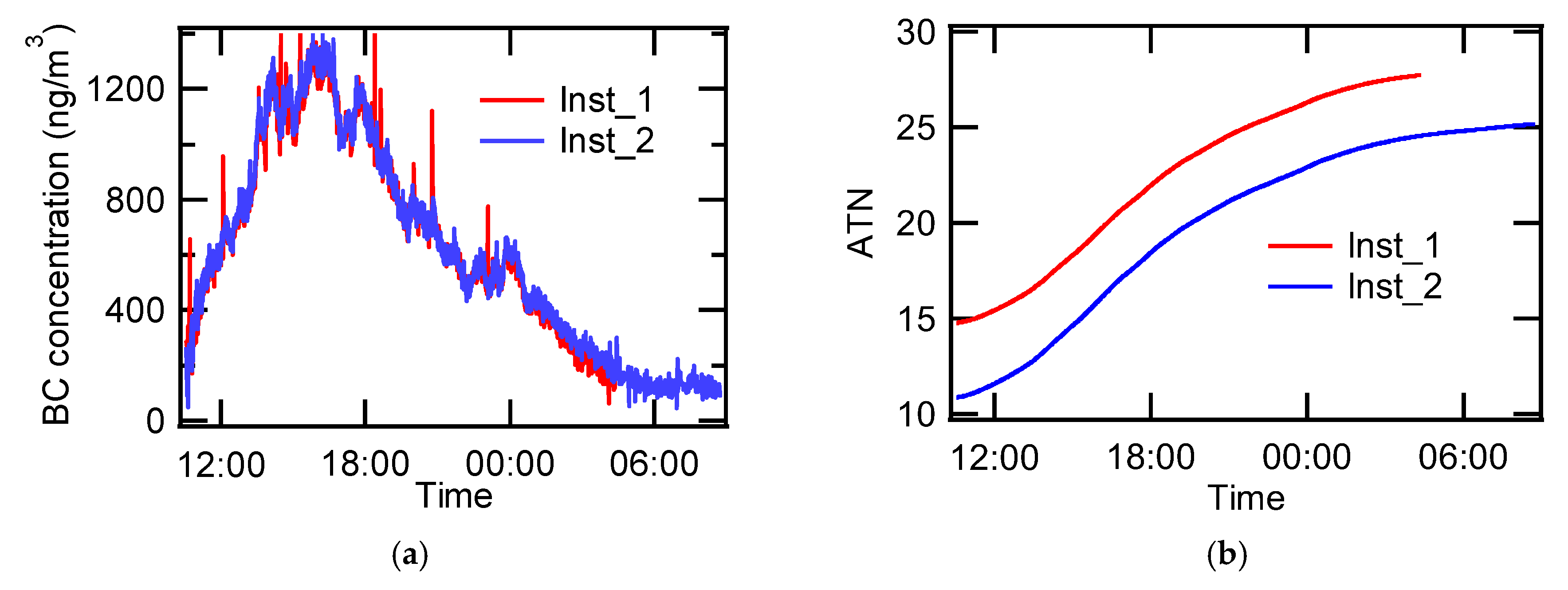
Figure 2 shows a typical BC concentration collected from two devices for indoor BC. The Inst_1 intermittently exhibits spike noises while the Inst_2 does not. The occurrence of intermittent spikes, however, was not reproducible. Sometimes, the Inst_2 exhibited more severe spike noises than Inst_1 does, implying that the noise was not device-dependent. Changes in ATN values for two devices are also shown in
Figure 2 as a function of time. Both devices show gradual increase in ATN values, meaning that the filter has been darkened by indoor aerosols. It is interesting to note that the initial ATN value is different from device to device. Even negative ATN value was reported in some cases for the initially installed clean filter though the initial negative ATN value does not affect the calculation of BC concentration [
1].
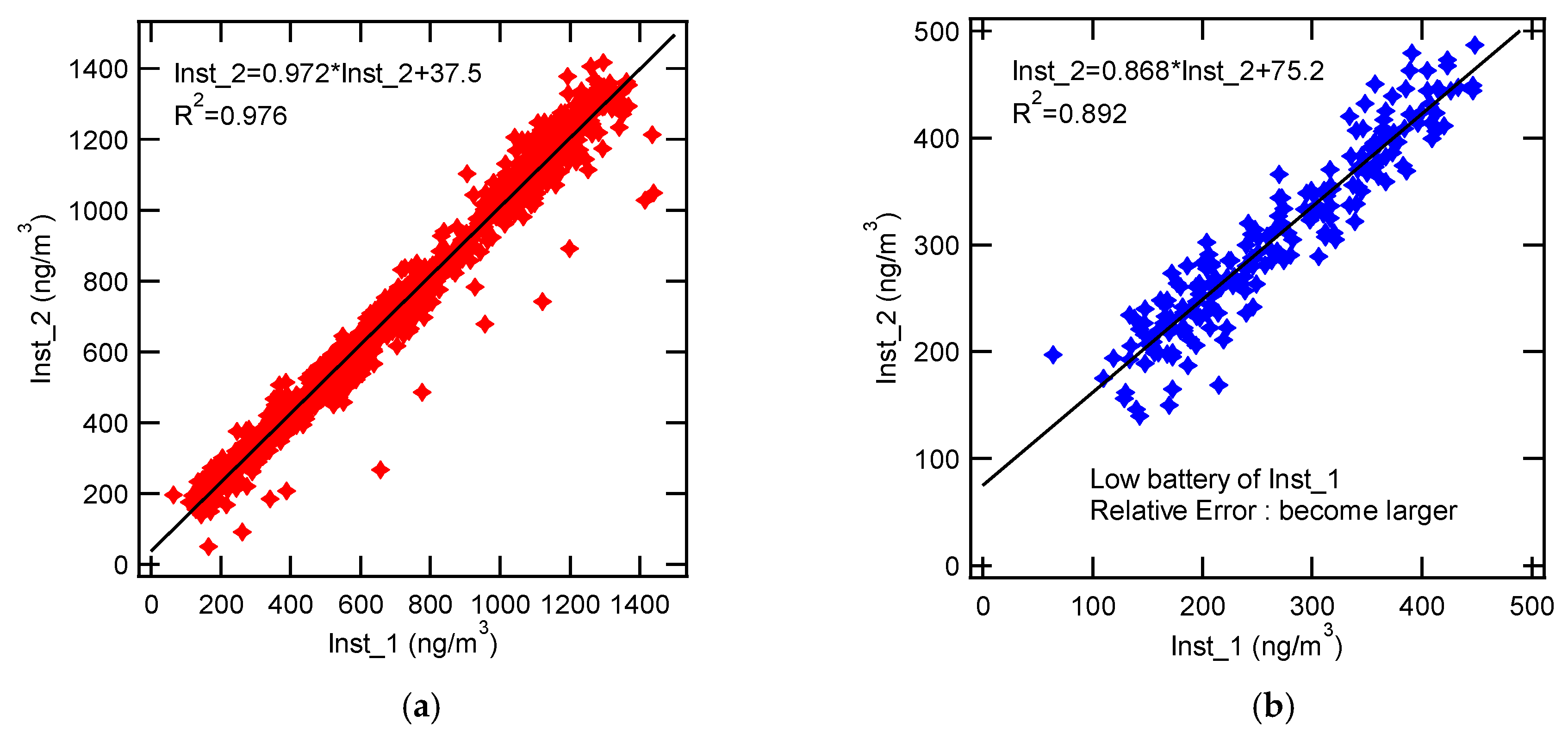
As can be seen in
Figure 3a, two devices show excellent agreement for the data shown in
Figure 2. The slope of the linear fitting curve for Inst_2 versus Inst_1 is 0.972. The coefficient of determination (R
2) is 0.976. However,
Figure 3b shows that the relative error between both devices becomes larger when the battery status of Inst_1 is lower than 0.8 (The battery status indicates 1.0 at full charge). Not only is the slope deviated from 1, but the coefficient of determination is also lower than the case where the battery status was higher than 0.8. The y-intersect is also higher than the case where battery status was over 0.8. Nominally, the error is expected to be larger than 10% at low battery status. Note that a similar test is needed with respect to Inst_2 to completely understand the effect of battery status on the performance of devices. Data collected at low battery status may need to be double-checked for assurance.
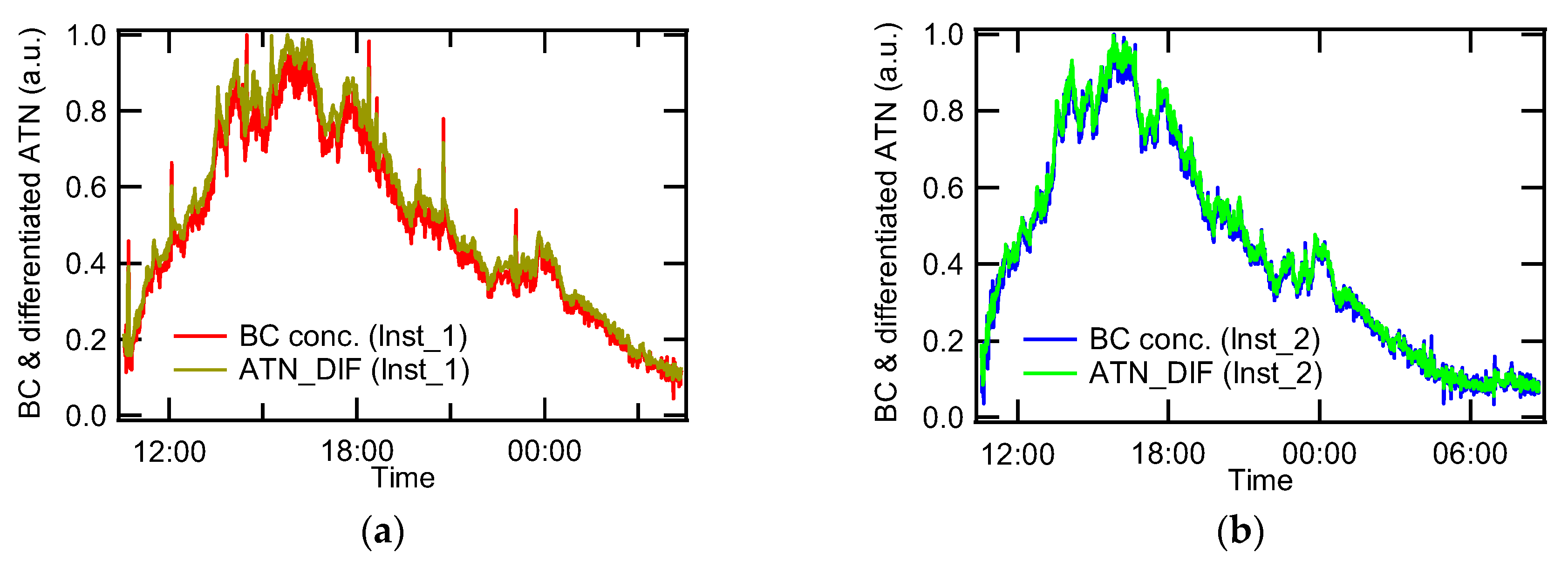
The process of obtaining BC concentration is as follows; (i) measurement of reference signal and sensing signal as inputs; (ii) calculation of ATN at time t using Equation (1); (iii) calculation of ATN at time
t+∆
t; (iv) calculation of ∆ATN using Equation (2); and (v) conversion of ∆ATN into BC concentration using Equation (3). As an attempt to reduce noise, we took a numerical derivative of ATN. We observed that the time series of the numerical derivative of ATN showed very nice similarity to BC concentrations, as can be seen in
Figure 4. Furthermore, the intensity of intermittent spikes decreased for both Inst_1 and Inst_2. Statistical result for about 17–20 h measurements shows that the level of standard deviation (1-σ) turned out to be basically the same. The recorded BC concentrations for Inst_1 and Inst_2 are 702 ± 337 ng/m
3 and 604 ± 378 ng/m
3, respectively. The normalized numerical derivatives of ATN for Inst_1 and Inst_2 are 0.522 ± 0.249 and 0.434 ± 0.271, respectively. As for Inst_1, the ratio of the standard deviation to the average BC concentration is calculated to be 0.480 and the ratio of the standard deviation to the average numerical derivative of ATN is to be 0.477. As for Inst_2, the ratio of the standard deviation to the average BC concentration is calculated to be 0.626 and the ratio of the standard deviation to the average numerical derivative of ATN is to be 0.625. It turned out that there was no significant difference between the recorded BC concentration and the derivative of ATN for entire measurement period. However, it was quite effective to take a derivative of ATN signal when the spike noise happened. Truncation error may be added when the number of calculation step increases. The numerical derivative may help reduce the magnitude of spike noise because less truncation errors were involved during the conversion process of
I into BC concentration by directly obtaining the derivative of ATN. One of the recommendations to improve detection limit for the manufacturer might be to introduce a differentiation function on the circuit board of the device and to directly acquire the derivative value as an alternative to the ∆ATN.
3.1. Amplified Noise Relating to Power Source
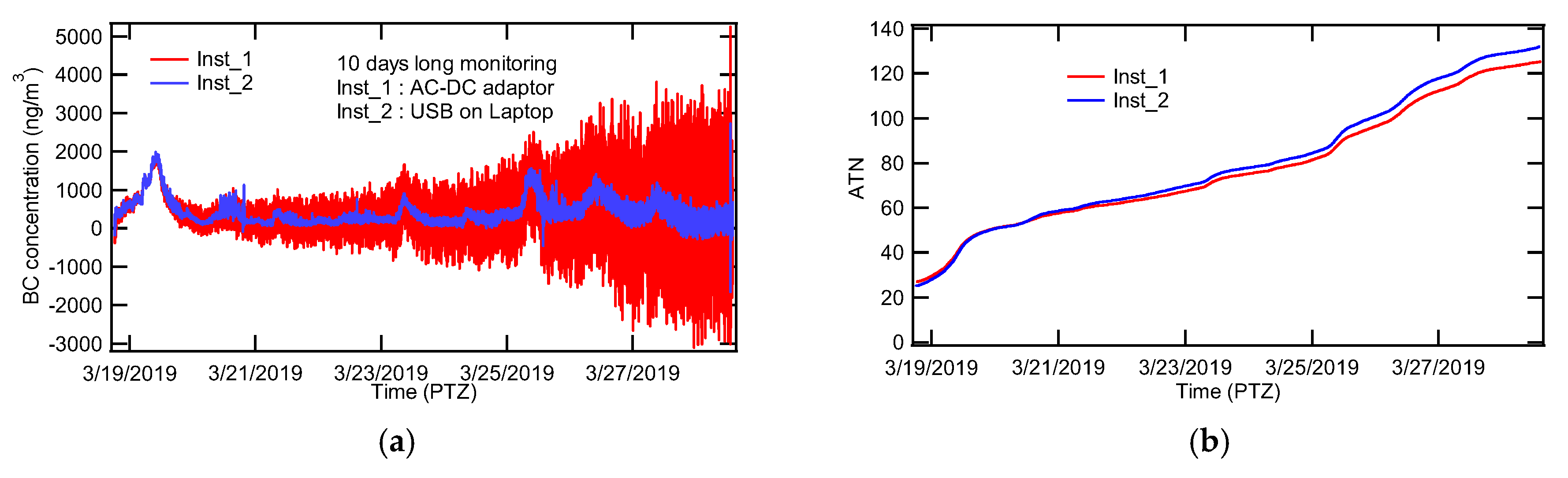
As shown earlier, the internal battery lasted only about 20 h. For this reason, Inst_1 was plugged to an AC-DC adaptor while Inst_2 was connected to a USB port on a laptop for the monitoring longer than 20 h.
Figure 5 shows the comparison between Inst_1 and Inst_2 for the measurement of indoor BC concentration approximately 10 days long without changing a filter. The author did not replace the filter intentionally, in order to observe the effect of overloading on the BC measurement. Unexpectedly, noise of Inst_1 gradually increased and was significantly amplified until the end of the test. The noise of Inst_1 started to increase after approximately 18 h since the beginning of measurement. The “18 hours” is similar to the duration of internal battery of Inst_1. It is thought that this noise was associated with a process of AC to DC conversion. As soon as the Inst_1 consumed up the internal battery, it started to depend on the AC-DC adapter to charge the internal battery. At this moment, the noise of AC seemed to be transferred to the input circuit of Inst_1. The ATN of Inst_1 was larger than that of Inst_2 in the beginning of the comparison measurement though it was reversed at the end of the test. The difference of ATN between the start and the end of the test ought to be same if the other conditions remain same. However, as can be seen in
Figure 5b, the difference of ATN between Inst_1 and Inst_2 definitely exists, implying that some factors of Inst_1 are different from those of Inst_2. The factor could be the difference in the sampling flow rate, the sensitivity of photodiode, the power of the light source, and the efficiency of optics module. The author may refer it to a “system response factor”. If the system response factor is evaluated before manufacturing, calibration for the device will become more robust. It is intriguing that Inst_2 also becomes noisy around Mar. 24 when ATN value reaches 80. It is better for users to replace the filter before ATN reaches 80 in order to acquire reliable data.
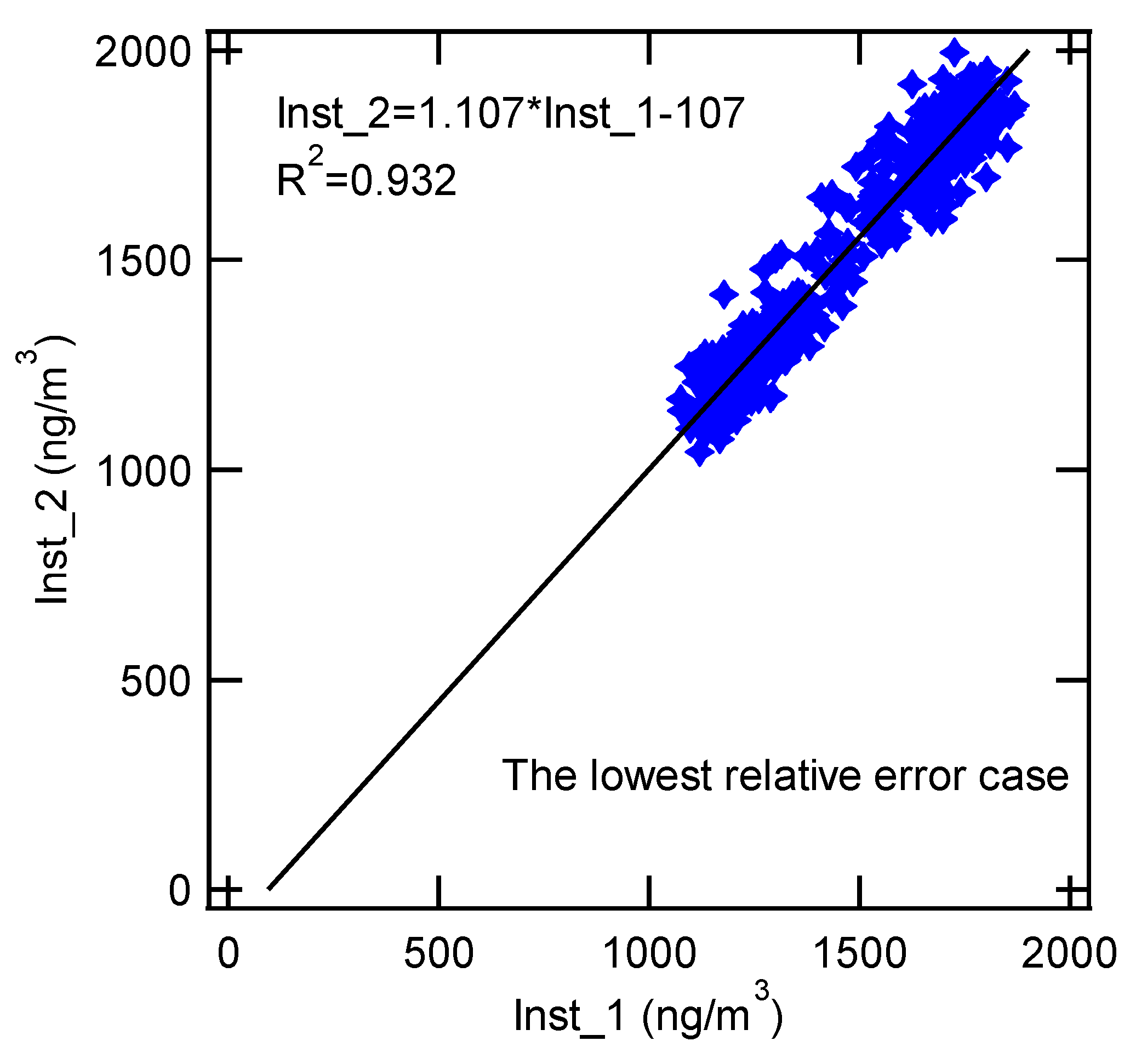
Figure 6 displays the comparison between Inst_1 and Inst_2 for the case where the relative error is low in the 10 days long term comparison. The correlation is still good enough to be used as a BC sensor, though Inst_2 is slightly overestimated with respect to Inst_1. Inst_1 was selected as a reference in the present study because it has shown more stable performance than Inst_2 since its purchase. In addition, Inst_2 has sporadically failed in collecting data for the sampling flow rate settings except 0.1 lpm.
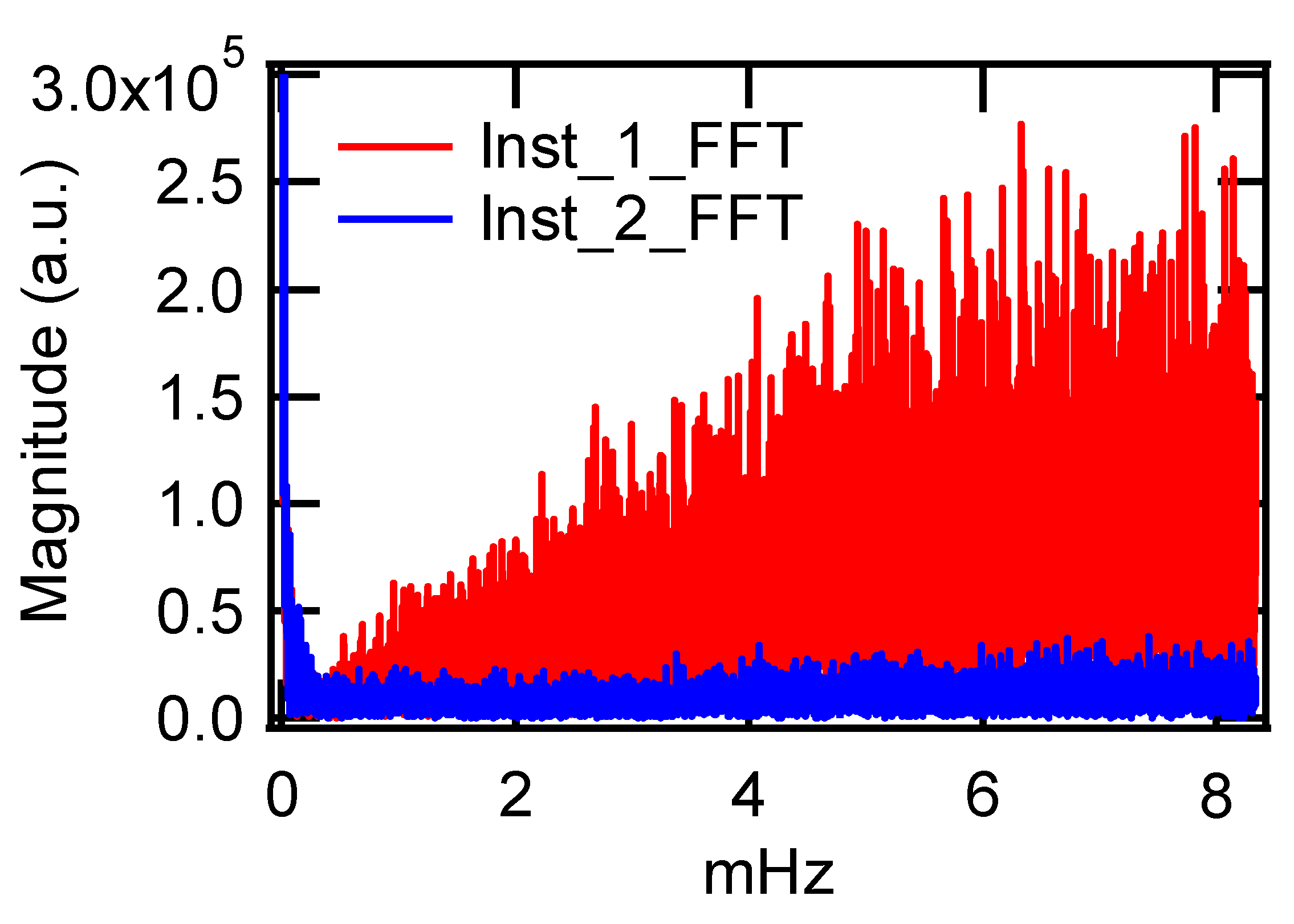
In order to analyze the origin of the intensified noise in BC concentration, an analysis using a Fast Fourier Transform (FFT) was performed for the BC data measured every 1 min.
Figure 7 demonstrates that Inst_2 did not pick up a signal at most frequencies but the noise was induced from all frequencies for Inst_1. FFT results show that Inst_1 suffered noise intrusion at all frequency domain of interest.
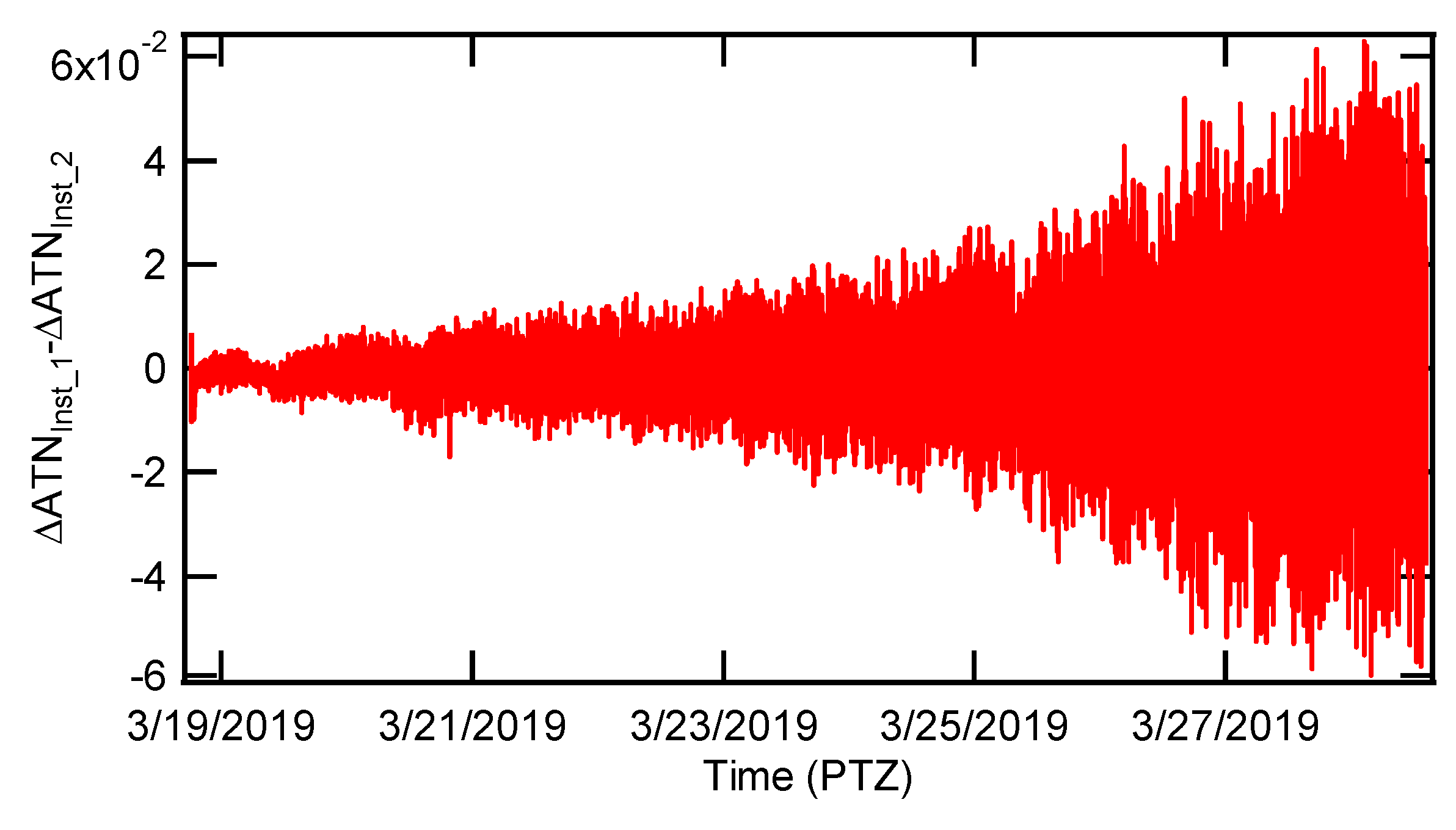
Figure 8 shows that the difference of ∆ATN between Inst_1 and Inst_2 fluctuates gradually. Not only do the absolute values for the difference between ∆ATN
Inst_1 and ∆ATN
Inst_2 become larger, but the ∆ATN values also exhibit negative values which are trivial and do not contain any physical meaning. The envelope of the difference of ∆ATN between Inst_1 and Inst_2 increases until the end of the test. It would have increased gradually if the test had continued. It appears that not only the connection to an AC-DC adapter but also the filter-overloading effect, or the combination of both, could contribute to the amplification of noise.
3.2. Zero Test Using Filtered Clean Air
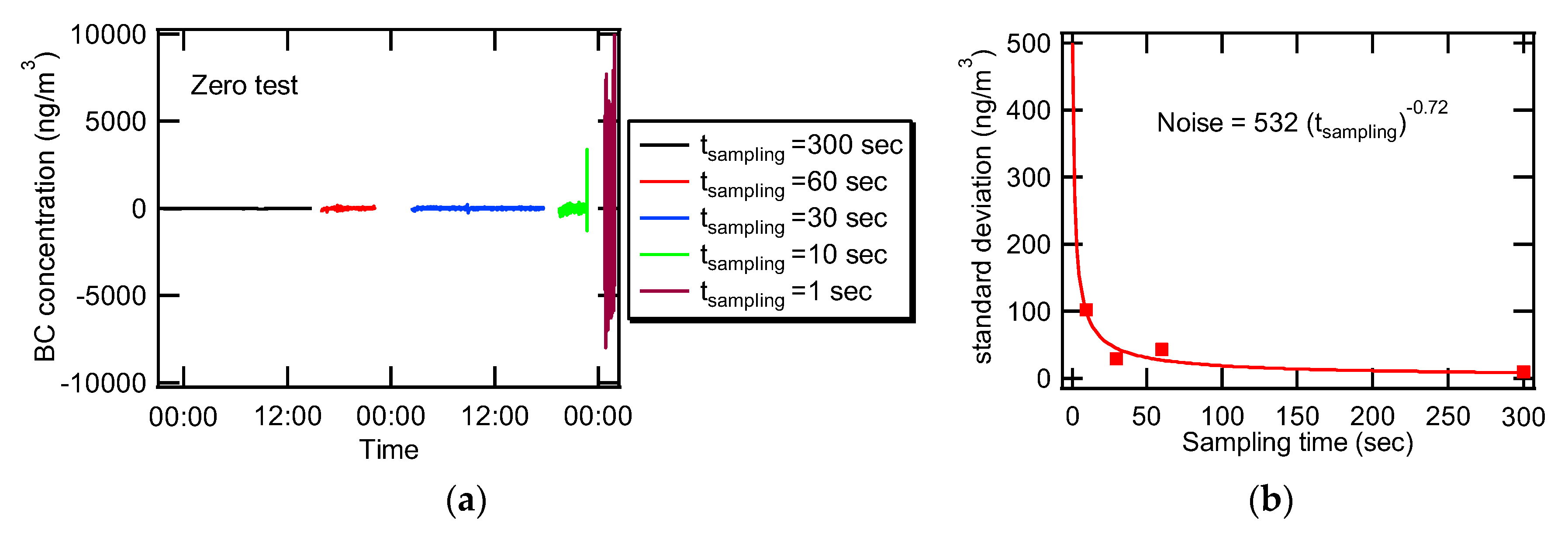
The zero test was performed to validate the noise levels at different sampling time settings. BC concentrations for filtered clean air are shown in
Figure 9. Noise levels were acceptable to the measurement of BC at low concentrations except when the sampling time was 1 s. Note that the variation of BC concentrations at 1 s of sampling time is 10 times higher than those for 30, 60, and 300 s. For further analysis, standard deviations (error) of BC concentrations at each sampling time settings were plotted versus the sampling time, and a curve fitting between the standard deviations and the samplings time was performed using a power law relation. According to Equation (3), the noise levels increase as the sampling time gets shorter and it is not unreasonable to infer that the power would be −1. However, the power in this present study turned out to be −0.72, which means that there are other sources of noise generation. Presumably, a drift in ATN exists similarly to the case of AE-31 which is an instrument for monitoring BC continuously and operates with a principle similar to AE51 [
7].
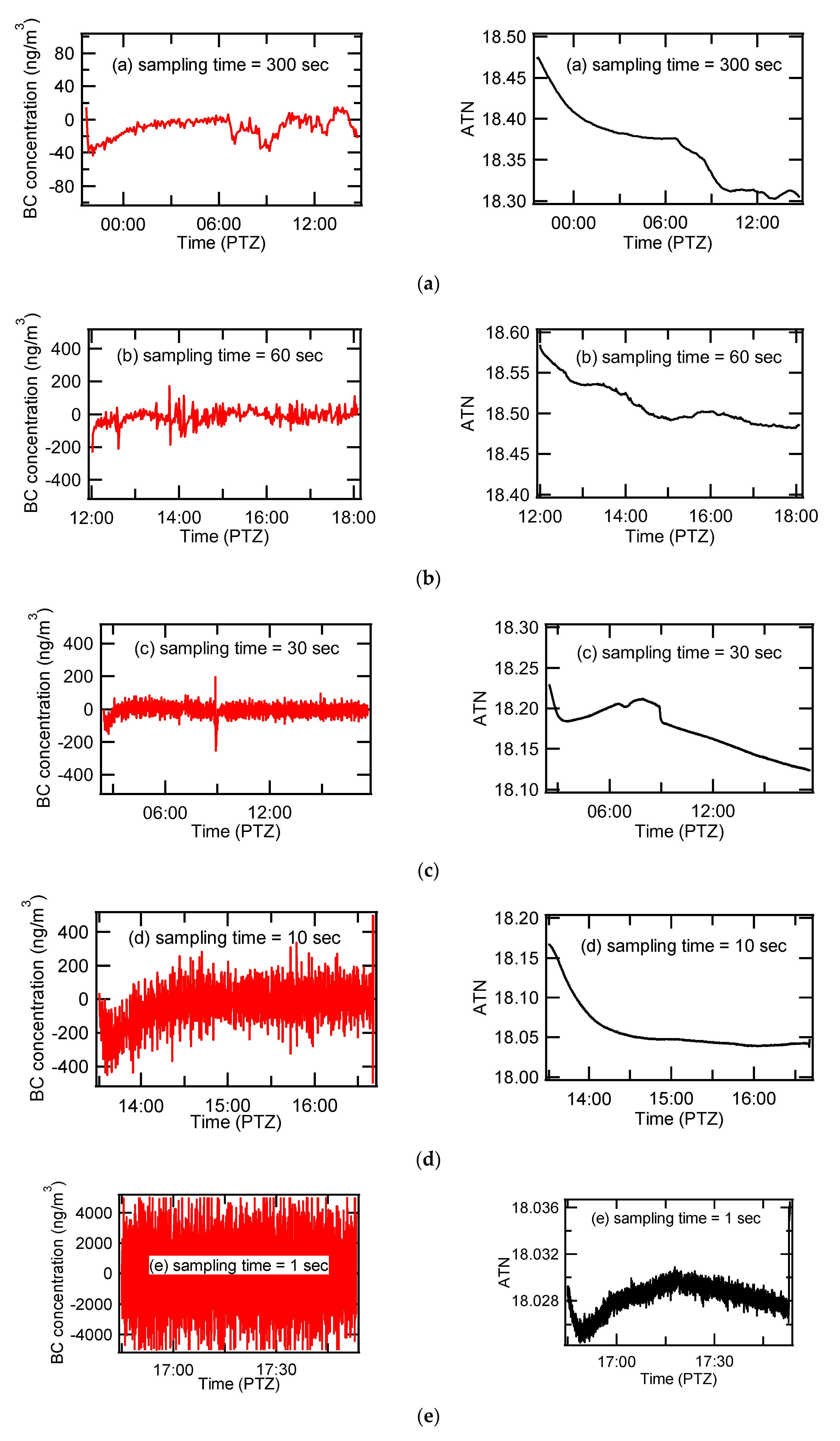
Figure 10 presents BC concentrations and the variations of ATN for filter-cleaned air at different sampling time settings. Errors get bigger as the sampling time gets shorter. It is worthwhile to note that BC concentrations turned out to be near zero in average, though real-time negative values were present for all the different sampling time settings. One of the unexpected features in the present performance test is that the ATN values varied even though particle free air was introduced into the device.
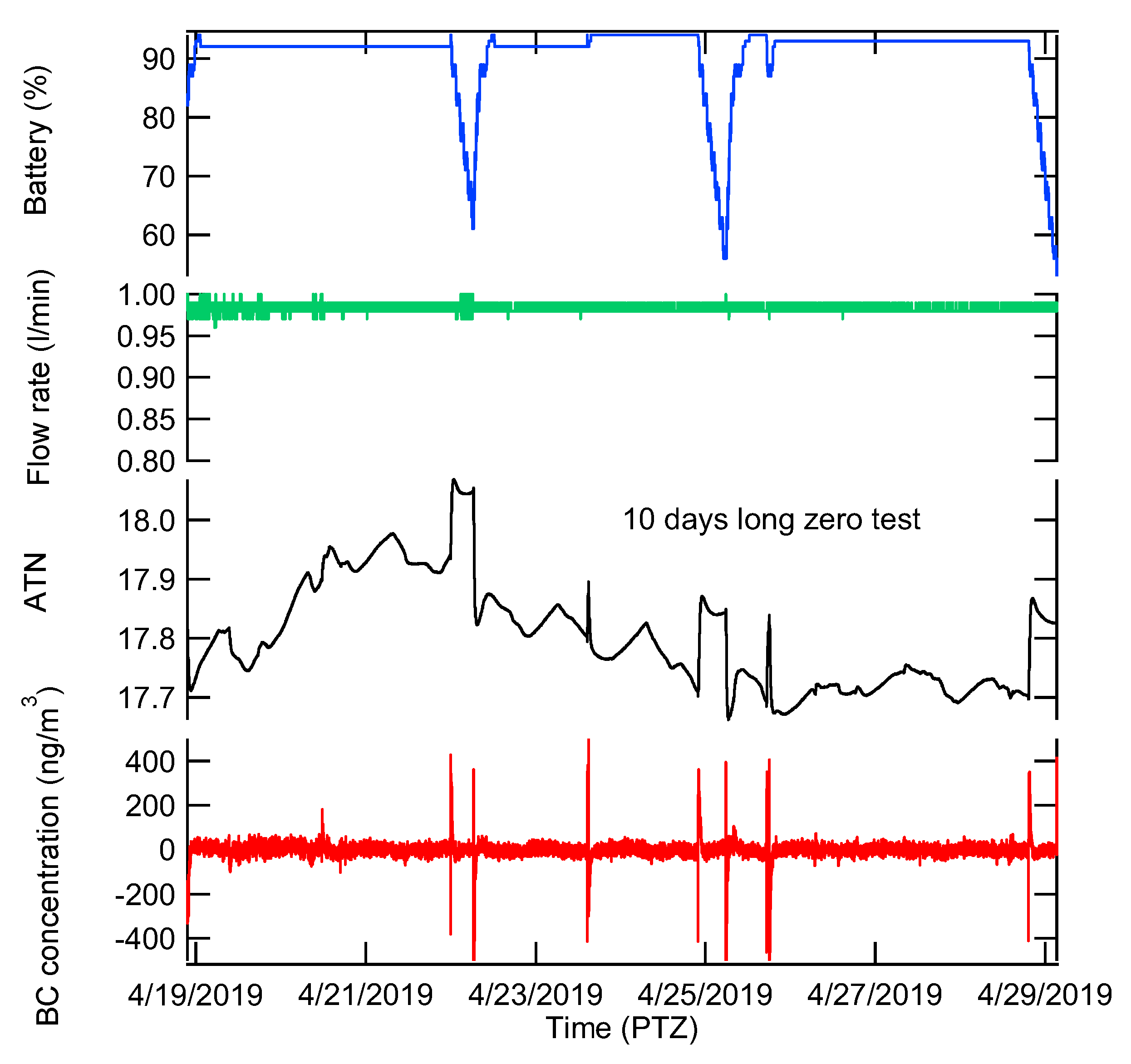
Figure 10 clearly shows that ATN nominally decreased for all the sampling time settings though ATN should be constant for particle free air. In order to further investigate the decreasing tendency in ATN as a function of time, the zero test was performed for 10 days under the condition where the sampling time was set to 60 s and the sampling flow rate was 0.1 lpm. These settings were the most stable among other setting values. As already investigated, the battery lasts only about 20 h. To test longer than 20 h, we used two auxiliary battery packs which are frequently used for charging smartphones and tablets. For the entire data collected for 10 days, the average concentration was −0.011 ng/m
3 and the standard deviation was 46.9 ng/m
3. These values are similar to those obtained during the short term zero test performed for 6 h. Generally, microAeth
® AE51 performs extremely well, as it should. The concentration overshot occasionally due to the sudden changes in ATN, which was probably caused by the battery status. As can be seen in
Figure 11, an auxiliary battery charged the internal battery installed in a device from around 80% up to full charge status as soon as the auxiliary battery was connected to the device. Then the auxiliary battery was used as a power source as long as it drained until Apr. 22. As soon as the auxiliary battery ran short of its power, the fully-charged internal battery started to be used as a power source. ATN changed subsequently on the moment when the power source was switched from the auxiliary battery into the internal battery with the auxiliary battery being connected to the device. Sudden changes in flow rate might cause abrupt variation in BC concentration because one of the variables to determine BC concentration is the flow rate.
Figure 11 shows that the flow rate varied within ±2% of a setting value for 10 days. The flow rate was maintained nearly constant independent on the battery status and on the switching moment of power sources. Consequently, it was demonstrated that the ATN drastically changed when the power source was altered. Changing power sources from one auxiliary battery to another one created sudden changes of ATN, resulting in spikes of BC concentrations. It took about 30 min to 2 h for the sudden spikes in BC concentration to disappear. It is recommended that users should start measurements with fully charged status and keep operating until the internal battery is drained without connecting to any external power source. For longer measurement, the auxiliary battery needs to be plugged to the fully charged device. Careful selection of power sources leads to the exclusion of unwanted noise.
One of interesting results regarding ATN is that ATN is not constant for particle-free air. Rather, ATN fluctuates up and down. The increase in ATN for particle-free air was reported for some AE31s during the monitoring for 13 days [
7]. The decrease in ATN for particle-free air toward microAeth
® AE51 during 10 days of monitoring was observed in the present study for the first time, as far as the author knows. The unsteady variation of ATN might be due to the deposition of light-absorbing particles caused by leaks at flow channel or the deposition of light-scattering particles which might penetrate through the particle-removal filter. The decrease in ATN shown around 22:00 to 02:00 in
Figure 10a matches well with the negative BC concentrations shown in the same time frame. In fact, the ATN readings do correspond to the BC concentrations though the non-uniform ATN appears to have nothing to do with the BC concentrations. The decrease in ATN consequently results in negative BC concentration, which is physically meaningless, as already mentioned. This is an additional issue other than the noise amplification. The negative concentration seems partly due to a compensation scheme which forcedly displays zero concentration under nearly zero concentration condition. One of these schemes is probably an averaging scheme, which is simple to apply to the instrument circuit.
3.3. Uncertainty Propagation Analysis
The microAeth
® AE51 assumes a constant attenuation cross section, so the first term of inside square root of Equation (5) goes to zero. The spot area also ought to be constant but it could be changed due to leakage from failed sealing on the contact between the filter and the conduit. The spot size can be measured using a magnifier or digital image analysis, but the uncertainty of the spot size was assumed to be 2% [
7]. Uncertainty of the flow rate may ensue not only from the stability of a flow controller but also that of a pump. The uncertainty of a flow controller could be 1.5%, as assumed by Backman et al. [
7] and the uncertainty of a pump may be 5% [
20]. We liberally assume the uncertainty of the flow rate as 5%, which includes only the uncertainty of a pump. The uncertainty of the measurement time should be zero. However, we noticed that a time lag occurred after the 10-day-long measurement. At the beginning of the test, the clock of the device was synchronized with the clock in the laptop computer used for data collection. At the end of the test, however, the clock of the device lagged behind 30 s. Thus, we can assume that the uncertainty of time is non zero, though it is a very small number. The time lag divided by the entire measurement duration (10 days) is calculated to be 3.47 × 10
−3%. The last term of the inside square root of Equation (5) may dominate overall uncertainty.
Here, we can assume
and
because the reference signal and sensing signal do not change much during the time interval especially when the sampling time is not long. Thus, the last term inside square root of Formula (5) can be written as below.
Incorporating Equation (5) and formula (6) gives us the following Equation.
The error of reference signal (δI0/I0) and that of sensing signal (δI/I) can be estimated from the collected raw data. The errors of reference signal and sensing signal were calculated by dividing the standard deviations (1-σ) by the averages of the reference signal and sensing signal during entire measurement, respectively. The error of reference signal (δI0/I0) was estimated to be 0.3% and the error of sensing signal (δI/I) was estimated to be 0.3% or 4.3% for the filtered clean air and the indoor BC, respectively. Then, the overall uncertainty for indoor BC is calculated to be 8%. The overall uncertainty for the filtered clean air must be smaller than 8% because the error of sensing signal for the filtered clean air is smaller than that for the indoor BC.


