Estimating Road Segments Using Kernelized Averaging of GPS Trajectories

Abstract

A method called iTEKA, which stands for iterative time elastic kernel averaging, was successfully used for averaging time series. In this paper, we adapt it to GPS trajectories. The key contribution is a denoising procedure that includes an over-sampling scheme, the detection and removal of outlier trajectories, a kernelized time elastic averaging method, and a down-sampling as post-processing. The experiment carried out on benchmark datasets showed that the proposed procedure is effective and outperforms straightforward methods based on medoid or Euclidean averaging approaches.

1. Introduction

During the last decade, the development of navigational and geolocation systems and applications has experienced strong growth. For the associated services, such as human behavior analysis, traffic modelization and prediction, smart city information services, geo-localized and contextualized recommendation, etc., to be exploitable in urban areas, it is necessary to rely on an up-to-date cartography. However, maintenance of road and pedestrian network maps requires costly manual editing in time and money. This need has spawned a specific research theme around the development of automated extraction algorithms of road network maps from GPS trajectories [1,2,3]. Global Position Systems (GPS) trajectories are easily and cheaply collected using consumer embedded equipment, such as smart-phones. Unfortunately, they are in general noisy, mainly due to the sensitivity of the GPS tracking system that is used, but also due to the fluctuation, or loss, of the signal from the satellites. Consequently, in many places, such as in cities or mountain environments, due to reflections, magnetic interferences or even tropospheric conditions or sun activities, GPS trajectories can be erroneous (more than 10 m deviations) or characterized with missing data, making them unsuited for applications without dedicated preprocessing.

When a single trajectory is at hand, Kalman filtering [4] is usually the classical approach used to clean up this kind of sequential data. When, instead of a single trajectory, a set of trajectories can be considered, such as the random realization of a similar path followed by a population of pedestrians or road vehicles, one can consider ensemble filtering approaches such as ensemble Kalman filtering [5] or variant of particle filtering allowing to cope with historical data [6].

Both Kalman and ensemble Kalman methods require jointly the estimation of a measurement model and a dynamical model. However, the inference of these models are difficult to estimate with accuracy, specifically when the noise is non-Gaussian, and, furthermore, the parameters of the models may change with time and space, from one segment to the other.

In this article, we address the problem of cleaning sets of pedestrian or vehicle GPS trajectories corresponding to a road segment without making any assumption on the noise or the nonlinear dynamics underlying the movement of the tracked object. The cleaning procedure that we present relies on an ensemble filtering algorithm for sets of trajectories mostly based on the notion of centroid defined for a subset of time series. It involves five steps, as depicted in Figure 1:

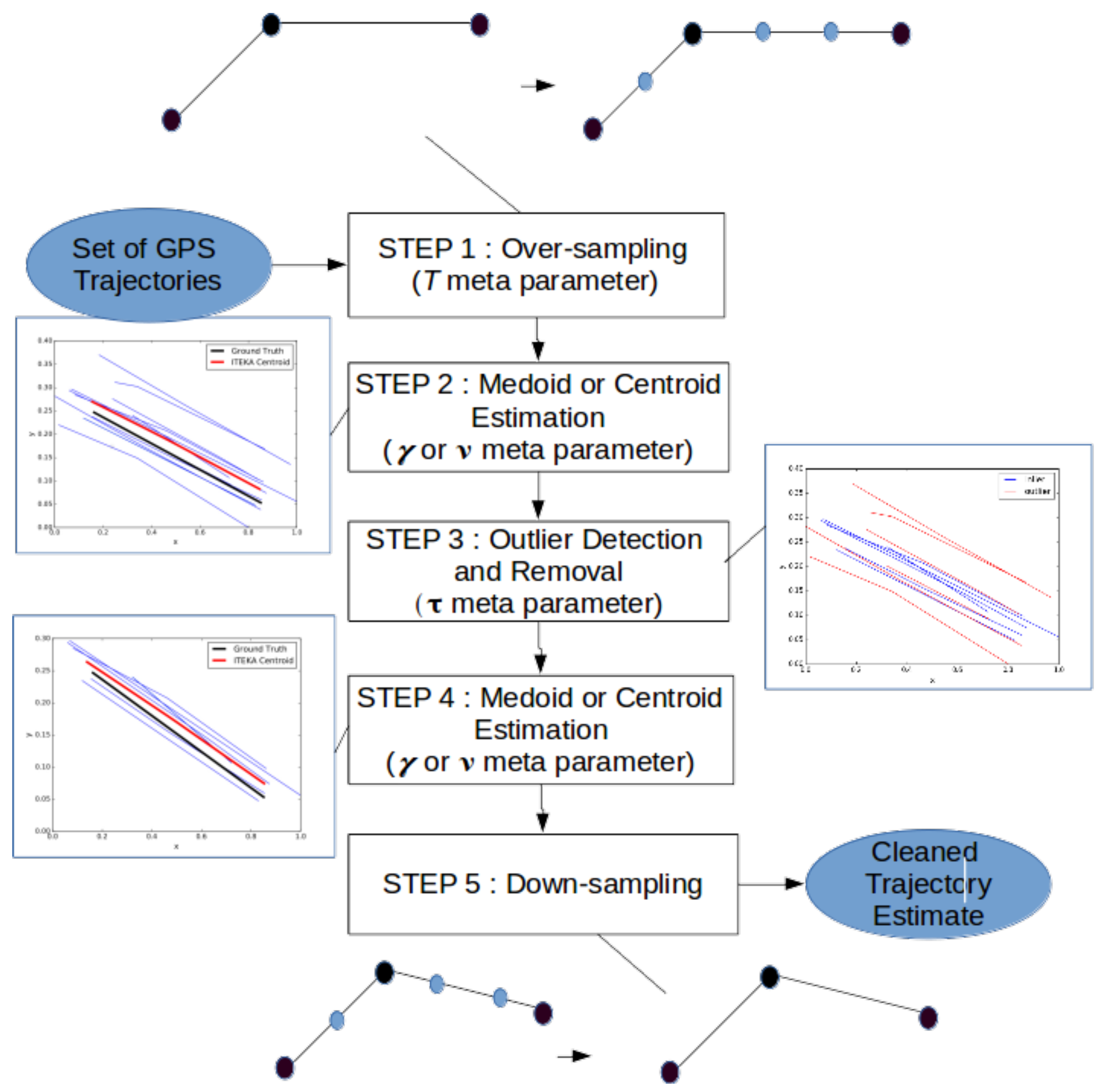
• an over-sampling of the trajectories such that they all share a higher sampling rate, namely they are described with the same higher number of samples (Section 3.1);
• a first extraction/estimation of a medoid/centroid for a subset of GPS trajectories (Section 2.4 and Section 3.2);
• anomaly (outlier) detection and removal (Section 3.2);
• a second extraction/estimation of a medoid/centroid for a subset of GPS trajectories (Section 2.4 and Section 3.2); and
• a final down-sampling to reduce the sampling precision of the trajectories down to the average sampling precision of the initial set of trajectories (Section 3.3).

This overall cleaning procedure was used during our experimentation to test comparatively various methods from the state of the art. We evaluated: (i) four medoid methods based on the Euclidean distance, the well-known dynamic time warp (DTW) measure [7,8], the soft version of DTW (soft-DTW, [9]) or a kernelization version of DTW (${\mathcal{K}}_{\mathrm{rdtw}}$,10]); and (ii) four centroid based methods, namely the Euclidean centroid [11], the DTW Barycenter Averaging (DBA) centroid according to the method proposed in [12], the soft-DTW centroid developed by Cuturi and Blondel [9] and the iterative Time Elastic Kernelized Averaging proposed (iTEKA) in [13].

Section 2 introduces the main concepts that are behind the DTW time elastic measure and its kernalization. It also introduces the general purpose (iterative Time Elastic Kernel Averaging (iTEKA) procedure that has been specifically developed to average sets of time series. Section 3 addresses the averaging of sets of GPS trajectories. It details mostly the preprocesing and postprocessing steps as well as the trajectory outlier detection and removal stage. Section 4 presents an experimentation carried out in the context of the “Averaging GPS segments Competition” (https://cs.uef.fi/sipu/segments/) [14] proposed by University of Eastern Finland. A conclusion ends this study.

2. From Dynamic Time Warping to Time Elastic Kernels Averaging

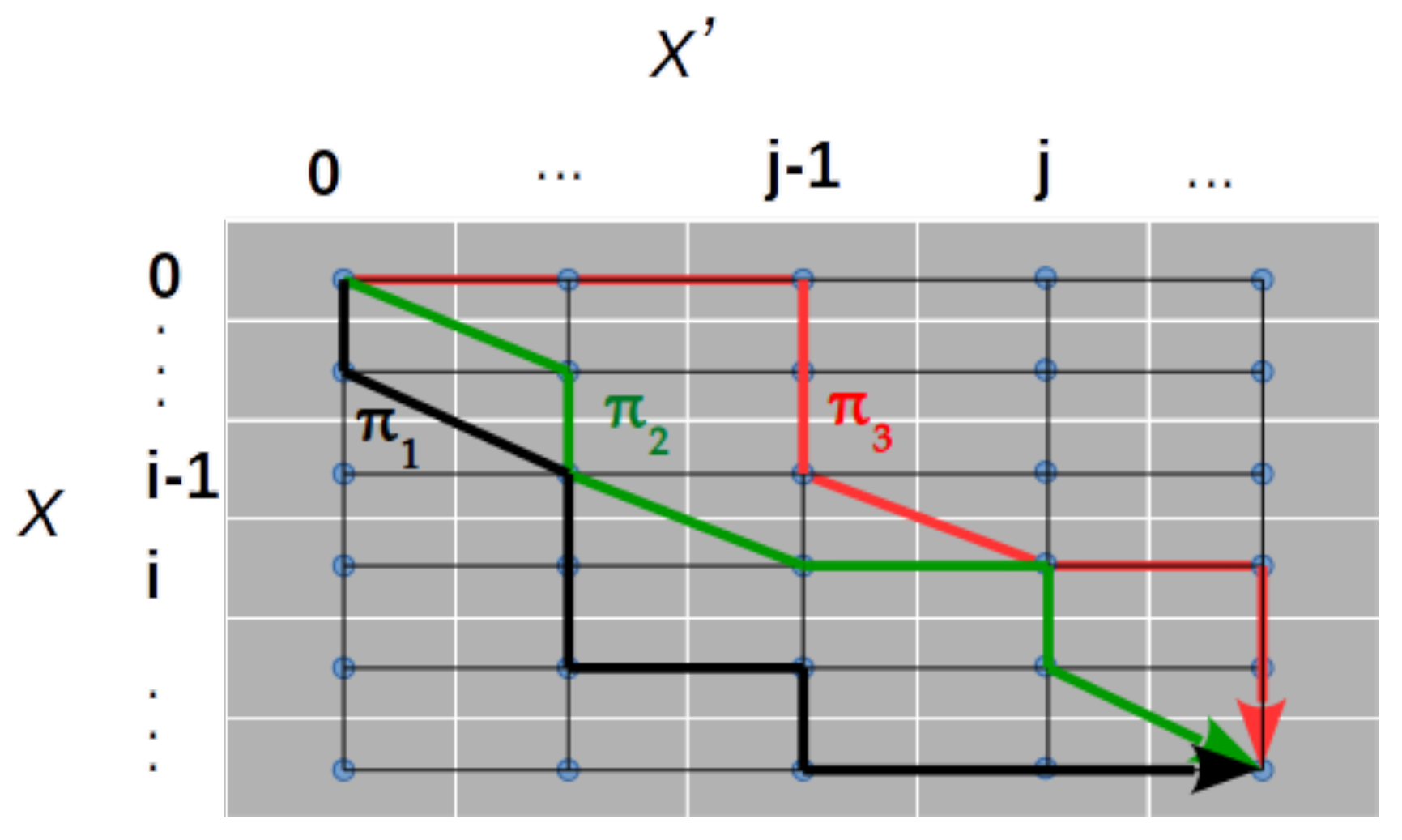
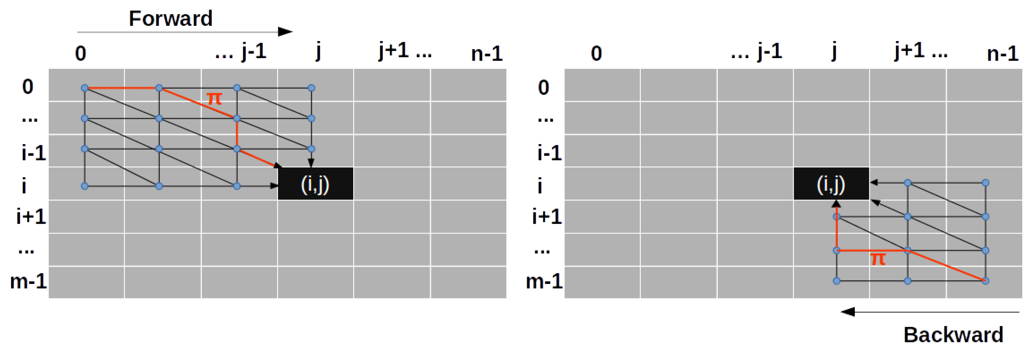
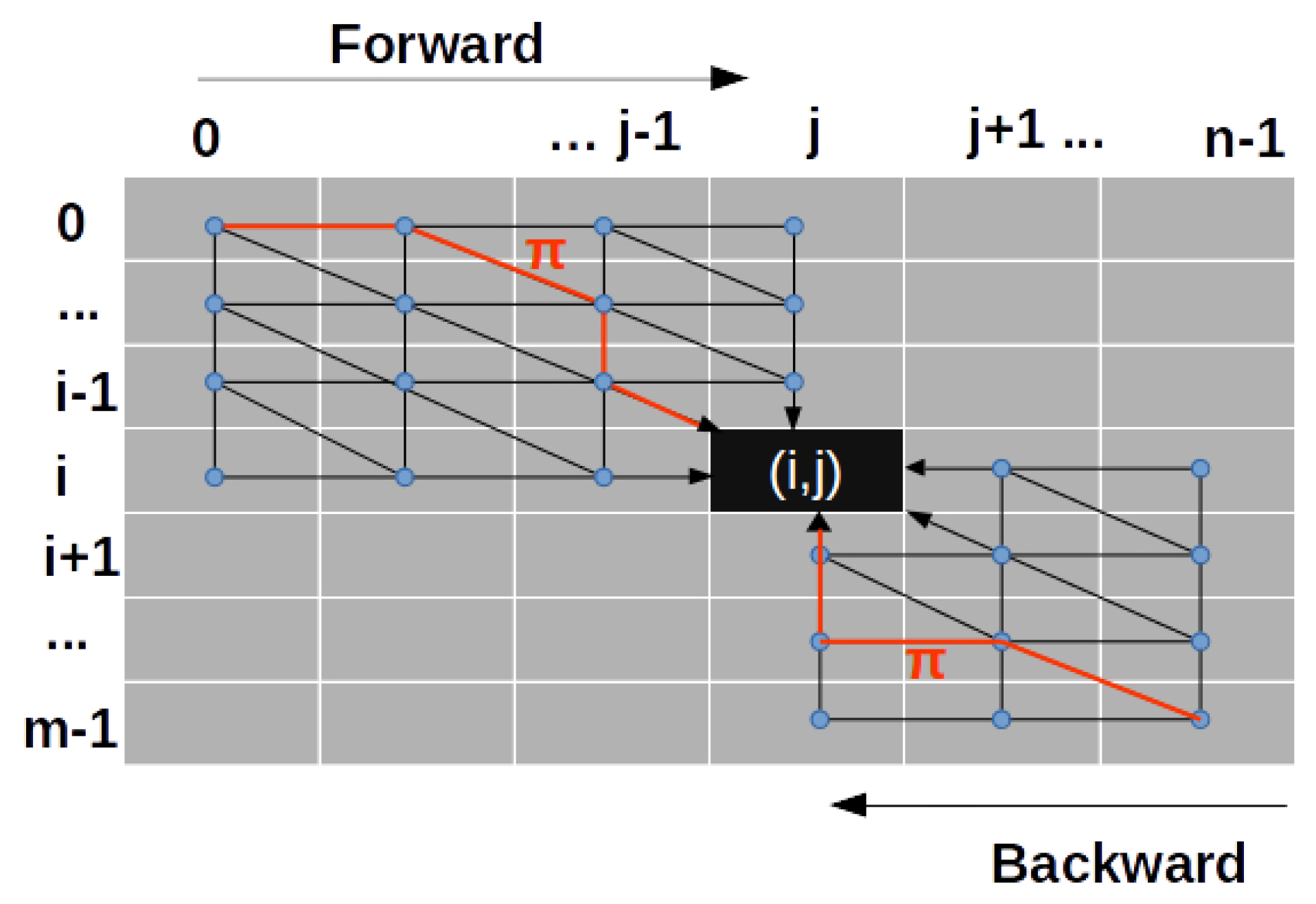
2.1. Dynamic Time Warping

Dynamic Time Warping (DTW) was introduced in [7,8] as a measure of similarity between time series. DTW similarity is the results of an optimal alignment path ${\pi }^{\ast }$ between a pair of time series (originally speech waves) while locally considering expansion or squeezing of the time line. An alignment path $\mathit{\pi }$ of length $\left|\mathit{\pi }\right|=m$ between two time series $\mathbf{x}$ and ${\mathbf{x}}^{\prime }$ is defined as the sequence of m ($max\left(\right|x|,|x^{\prime }\left|\right)\le m\le \left|x\right|+|x^{\prime }|$) pairs of aligned time stamps:

$$\mathit{\pi }=[({\pi }_1\left(0\right),{\pi }_2\left(0\right)),({\pi }_1\left(1\right),{\pi }_2\left(1\right)),...,({\pi }_1(m-1),{\pi }_2(m-1))]$$

where $({\pi }_1\left(k\right),{\pi }_2\left(k\right))$ means that $x_{{\pi }_1\left(k\right)}$ and $x_{{\pi }_2\left(k\right)}^{\prime }$ are aligned. ${\pi }_1$ and ${\pi }_2$ obey the boundary and monotonicity conditions as:

$$0={\pi }_1\left(0\right)\le {\pi }_1\left(1\right)\le ...\le {\pi }_1(m-1)=\left|x\right|-1$$

$$0={\pi }_2\left(0\right)\le {\pi }_2\left(1\right)\le ...\le {\pi }_2(m-1)=\left|x^{\prime }\right|-1$$

and, $\forall l\in \{0,\dots ,m-1\}$,

$$\begin{array}{ccc}\hfill {\pi }_1(l+1)\le {\pi }_1\left(l\right)+1\mathrm{and}{\pi }_2(l+1)\le {\pi }_2\left(l\right)& +& 1,\hfill \\ \hfill ({\pi }_1(l+1)-{\pi }_1\left(l\right))+({\pi }_2(l+1)-{\pi }_2\left(l\right))& \ge & 1\hfill \end{array}$$

The eligible alignments paths are classically represented in a $\left|x\right|\times |x^{\prime }|$ grid, as displayed in Figure 2.

Let $\mathcal{A}$ be the set of all possible alignments between two time series. The DTW similarity measure between time series $\mathbf{x}$ and ${\mathbf{x}}^{\prime }$ is thus defined as:

$$\begin{array}{c}\hfill \mathrm{DTW}(\mathbf{x},{\mathbf{x}}^{\prime })=\underset{\pi \in \mathcal{A}}{min}\sum _{\begin{array}{c}(t,t^{\prime })\in \pi \end{array}}\phi (x_t,x_{t^{\prime }}^{\prime })\end{array}$$

(1)

where $\phi :\mathbb{R}\times \mathbb{R}\to {\mathbb{R}}^{+}$ is a local distance measure (usually the Euclidean norm is used) on the set of real numbers $\mathbb{R}$.

2.2. Time Elastic Kernels

From the DTW formulation, several attempts have been made to build kernel measures more suitable for machine learning purpose, in particular in the context of support vector machine. Distance substituting kernels were first introduced [15,16], and, although such kernels are not definite positive, they have shown mixed success.

Later, the global alignment kernel was introduced [17], which is, in most practically encountered conditions, positive definite (${\mathcal{K}}_{\mathrm{ga}}$), and takes the following form:

$$\begin{array}{c}\hfill {\mathcal{K}}_{\mathrm{ga}}(\mathbf{x},{\mathbf{x}}^{\prime })=\sum _{\pi \in \mathcal{A}}\prod _{\begin{array}{c}(t,t^{\prime })\in \pi \end{array}}\kappa (x_t,x_{t^{\prime }}^{\prime })\end{array}$$

(2)

where $\kappa (.,.)=exp(-\gamma ·||.,.|{|}^2)$ is a local kernel and $\mathcal{A}$ is the set of all admissible alignment paths.

Marteau and Gibet [10] proposeda general procedure to construct positive definite time elastic kernels from general time elastic distances. In particular, ${\mathcal{K}}_{\mathrm{rdtw}}$, based on the design of a global alignment positive definite kernel for each single alignment path as given in Equation (3), has been defined such as close to the DTW matching scheme.

$$\begin{array}{c}\hfill {\mathcal{K}}_{\mathrm{rdtw}}(\mathbf{x},{\mathbf{x}}^{\prime })=\sum _{\pi \in \mathcal{C}\subset \mathcal{A}}{K}_{\pi }(\mathbf{x},{\mathbf{x}}^{\prime })\end{array}$$

(3)

where this time $\mathcal{C}$ is any symmetric (in the sense that, if C contains an alignment path $\pi$, C also contains the symmetric path of $\pi$) subset of the set of all admissible alignment paths $\mathcal{A}$ between two time series, and $K_{\pi }(\mathbf{x},{\mathbf{x}}^{\prime })$ is a positive definite kernel associated to the path $\pi$ and defined as:

$$\begin{array}{c}{\displaystyle K_{\pi }({\mathbf{x}}_i,{\mathbf{x}}_j)}={\displaystyle \prod _{\begin{array}{c}(t,t^{\prime })\in \pi \end{array}}\kappa (x_t,x_{t^{\prime }}^{\prime })}+{\displaystyle \prod _{\begin{array}{c}(t,t^{\prime })\in \pi \end{array}}\kappa (x_{t^{\prime }},x_t^{\prime })}\hfill \\ +{\displaystyle \prod _{\begin{array}{c}(t,t^{\prime })\in \pi \end{array}}\kappa (x_t,x_t^{\prime })}+{\displaystyle \prod _{\begin{array}{c}(t,t^{\prime })\in \pi \end{array}}\kappa (x_{t^{\prime }},x_{t^{\prime }}^{\prime })}\hfill \end{array}$$

(4)

with $\kappa$ a local kernel on ${\mathbb{R}}^d$. Typically, we use:

$$\kappa (a,b)=e^{-\nu ·\left|\right|a-{b\left|\right|}^2}\mathrm{with}(a,b)\in {\mathbb{R}}^2,$$

(5)

where $\nu$ is a meta parameter for this method.

Finally, soft-DTW [9], written as $dt{w}_{\gamma }$, was proposed to introduced a fully differentiable formulation from DTW. The essential idea is to replace the “hard” minimum operator by a “soft” expression that takes the following form with $\gamma \ge 0$ (which is a meta parameter for this method):

$$\begin{array}{c}\hfill mi{n}^{\gamma }\{a_1,\dots ,a_n\}:=\left\{\begin{array}{c}mi{n}_{i\le n}{a}_i,\gamma =0,\hfill \\ -\gamma ·log\left(\sum _{i=1}^n{e}^{-a_i/\gamma }\right),\gamma >0.\hfill \end{array}\right.\end{array}$$

(6)

It is easy to show that there exists a direct relation between the global alignment kernel ${\mathcal{K}}_{\mathrm{ga}}(.,.)$ and the soft-DTW: $dt{w}_{\gamma }(.,.)=-\gamma ·log\left({\mathcal{K}}_{\mathrm{ga}}(.,.)\right)$.

Soft-DTW is considered as a state-of-the-art method for averaging a set of time series. Hence, in our experimentation, we evaluated it as a baseline method that we plugged into Steps 2 and 4 of our processing pipeline.

2.3. Time Elastic Averaging of a Set of Time Series

The multiple alignments problem has been widely studied in bioinformatics [18]. It is known to be a NP-complete problem [19,20]. Due to the “hardness” of this problem, heuristics have been proposed to provide centroid estimates in a reasonable time.

Among others, an iterative heuristic approach was initially introduced by Hautamaki et al. [21] and popularized by Petitjean et al. [22] who introduced the DTW Barycenter Averaging (DBA) algorithm. The iterative procedure, which integrates three steps, is first initiated by selecting a reference time series r, usually the medoid of the set S of time series that is to be averaged. The best alignments for all the time series in S with r are evaluated during the second step. In the third step, the reference is updated by averaging all the samples that are aligned with the same sample of r. The two last steps are iterated until reaching a local minimum of the summation of the DTW distances between the time series in S and r.

The soft-DTW [9], which is fully differentiable in all of its arguments, has also been used to evaluate a centroid estimate for a set S of time series. Basically, in this case, the direct optimization problem can be solved using a gradient descent approach:

$$C=argmi{n}_x\sum _{i=1}^N=\frac{{\lambda }_i}{m_i}dt{w}_{\gamma }(x,y_i)$$

(7)

where $m_i$ is the length of time series $y_i$, ${\lambda }_i$ is a normalized weight associated to $y_i$ (${\sum }_i{\lambda }_i=1$), and C is the centroid we are seeking for. $dt{w}_{\gamma }(.,.)$ is constructed by replacing in dtw the min operator with a softmin operator that introduces the $\gamma$ meta parameter:

$$mi{n}^{\gamma }\{a_1,\cdots ,a_n\}\left\{\begin{array}{cc}\underset{i\le n}{min}{a}_i,\hfill & \gamma =0,\hfill \\ -\gamma log\sum _{i=1}^n{e}^{-a_i/\gamma },\hfill & \gamma >0.\hfill \end{array}\right.$$

(8)

These two time elastic averaging approaches (DBA and soft-DTW) constitute the state of the art in the context of averaging a set of time series.

2.4. Kernelized Time Elastic Averaging of a Set of Time Series

The averaging algorithm that we used to average a set of GPS trajectories is based on a probabilistic interpretation of the kernel alignment matrix (Equation (3)), as derived in [13]. This method is based on the recursive editing distance kernel, named REDK, which instantiates as ${\mathcal{K}}_{\mathrm{rdtw}}$ when DTW is considered as the editing distance.

The principle behind this interpretation is as follows. If we consider a stochastic alignment automata that, given two time series $\mathbf{x}$ and ${\mathbf{x}}^{\prime }$, provides alignment paths, $\pi$, according to a probability distribution $P_{\pi }\approx K_{\pi }$, then the cell $(i,j)$ of the kernel alignment matrix (Figure 3, left) corresponds to the sum of the probabilities of the paths that allow aligning the sub time series ${\mathbf{x}}_{0:i}$ and ${{\mathbf{x}}^{\prime }}_{0:j}$. The kernel alignment matrix can thus be understood as a forward probability matrix.

$${\mathcal{K}}_{\mathrm{rdtw}}({\mathbf{x}}_{0:i},{{\mathbf{x}}^{\prime }}_{0:j})\approx \sum _{\pi \in \mathcal{A}}{P}_{\pi }({\mathbf{x}}_{0:i},{{\mathbf{x}}^{\prime }}_{0:j})$$

(9)

Similarly, if we consider the backward alignment process (Figure 3, right), the cell $(i,j)$ corresponds to the sum of the probabilities of the paths that allow aligning backwardly the sub time series ${\mathbf{x}}_{\left|x\right|-1:i}$ and ${{\mathbf{x}}^{\prime }}_{|x^{\prime }|-1:j}$.

$${\mathcal{K}}_{\mathrm{rdtw}}({\mathbf{x}}_{\left|x\right|-1:i},{{\mathbf{x}}^{\prime }}_{|x^{\prime }|-1:j})\approx \sum _{\pi \in \mathcal{A}}{P}_{\pi }({\mathbf{x}}_{\left|x\right|-1:i},{{\mathbf{x}}^{\prime }}_{|x^{\prime }|-1:j})$$

Finally, if we consider the forward–backward $FB$ alignment matrix, as depicted in Figure 4, the cell $FB(i,j)={\mathcal{K}}_{\mathrm{rdtw}}({\mathbf{x}}_{0:i},{{\mathbf{x}}^{\prime }}_{0:j})·{\mathcal{K}}_{\mathrm{rdtw}}({\mathbf{x}}_{\left|x\right|-1:i},{{\mathbf{x}}^{\prime }}_{|x^{\prime }|-1:j})\approx {\displaystyle \sum _{\pi \in \mathcal{A}}}{P}_{\pi }({\mathbf{x}}_{0:i},{{\mathbf{x}}^{\prime }}_{0:j})·{\displaystyle \sum _{\pi \in \mathcal{A}}}{P}_{\pi }({\mathbf{x}}_{\left|x\right|-1:i},{{\mathbf{x}}^{\prime }}_{|x^{\prime }|-1:j})$ represents the sum of the probabilities of all the global alignment paths $\pi$ that cross cell $(i,j)$.

The forward–backward alignment matrix allows for the estimation of the expectation of the samples of ${\mathbf{x}}^{\prime }$ that are aligned with sample $x_t$ (given that $x_t$ is aligned) as well as the expectation of time of occurrence, $t^{\prime }$ of the samples of ${\mathbf{x}}^{\prime }$ that are aligned with $x_t$ as follows:

$$\begin{array}{c}E\left(x^{\prime }\right|x_i)\propto {\displaystyle \sum _{j=0}^{|x^{\prime }|-1}}{x^{\prime }}_j·\frac{FB(i,j)}{{\sum }_{j^{\prime }}FB(i,j^{\prime })}\hfill \\ E\left(t^{\prime }\right|x_i)\propto {\displaystyle \sum _{j=0}^{|x^{\prime }|-1}}j·\frac{FB(i,j)}{{\sum }_{j^{\prime }}FB(i,j^{\prime })}\hfill \end{array}$$

(10)

The expectation equations (Equation (10)) are at the basis of the procedure for averaging a set $\mathbf{X}={\left\{{}^k{x}_{0:T_k}\right\}}_{k=1\cdots N}$ of time series.

Let $r_{0:\left|r\right|-1}$ be a reference time series ($r_{0:\left|r\right|-1}$) that can be initially setup as the medoid of set $\mathbf{X}$. The centroid estimate of $\mathbf{X}$ is defined as the pair $(C,\mathcal{T})$ where C is a time series of length $\left|r\right|$ and $\mathcal{T}$ is the sequence of time stamps associated to the samples of C

$$\begin{array}{c}{C}_t=\frac{1}{N}{\displaystyle \sum _{k=1}^N}E\left({}^{k}x\right|r_t)\hfill \\ {\mathcal{T}}_t=\frac{1}{N}{\displaystyle \sum _{k=1}^N}E\left({}^{k}t\right|r_t)\hfill \end{array}$$

(11)

Equations (10) and (11) are at the basis of the iterative agglomerative algorithm, called iTEKA (iterative Time Elastic Kernel Averaging), that provides a refinement of the centroid estimation at each iteration until reaching a (local) optimum, as presented in Algorithm 1. This algorithm was used, among other state-of-the-art averaging algorithms such as Soft-DTW, in Steps 2 and 4 of the processing pipeline depicted in Figure 1.

Algorithm 1 Iterative Time Elastic Kernel Averaging (iTEKA) of a set of time series.

1: Let K be a time elastic kernel for time series satisfying a probabilistic interpretation Equation (9) 2: Let $\mathbf{X}$ be a set of time series of d dimensional samples 3: Let $C_0$ be an initial centroid estimate (e.g., the medoid of $\mathbf{X}$) of length n 4: Let $\mathcal{T}$ and ${\mathcal{T}}_0$ be two sequences of time stamps of length n initialized with zero values 5: Let $Mean{K}_0=0$ and $MeanK$ be two double values; 6: repeat 7: $C=C_0$, $\mathcal{T}={\mathcal{T}}_0$, $MeanK=Mean{K}_0$; 8: Evaluate $C_0$ and ${\mathcal{T}}_0$ according to Equation (11) //Average similarity between $C_0$ and elements of $\mathbf{X}$ 9: $Mean{K}_0$=$\frac{1}{\left|\mathbf{X}\right|}{\sum }_{\mathbf{x}\in \mathbf{X}}K(C_0,\mathbf{x})$ 10: until$MeanK\le Mean{K}_0$ 11: (C, $\mathcal{T}$) is the centroid estimation 12: Finally, uniformly re-sample C using the time stamps $\mathcal{T}$

An early version of iTEKA was first published on Arxiv site in 2015 [23].

3. Averaging a Set of GPS Time Series

3.1. Preprocessing the GPS Trajectories

Given a set $\mathbf{X}$ of GPS trajectory corresponding all to the same street or road segment, the averaging procedure presented previously cannot be used directly for several reasons:

• The street segment is not necessarily traveled in a single direction.
• The trajectories are traveled with variable speed, hence the trajectories are possibly not sampled with the same level of detail or uniformly.

The first preprocessing step (Step 1 in Figure 1) consists in realigning the trajectories such that they could be considered as being traveled in the same direction. If ${\mathbf{x}}_{0:n}\in \mathbf{X}$, we denote $\tilde{\mathbf{x}}$ the reversed trajectory, basically $\tilde{\mathbf{x}}={\mathbf{x}}_{n:0}$. The kernel defined in Equation (3) is used to reorganize $\mathbf{X}$.

This is achieved by selecting (randomly) one reference trajectory, $\mathbf{x}\in \mathbf{X}$ and for all ${\mathbf{x}}^{\prime }\in \mathbf{X}$, ${\mathbf{x}}^{\prime }\ne \mathbf{x}$, if ${\mathcal{K}}_{\mathrm{rdtw}}(\mathbf{x},{\mathbf{x}}^{\prime })\ge {\mathcal{K}}_{\mathrm{rdtw}}(\mathbf{x},\widetilde{{\mathbf{x}}^{\prime }})$, $\mathbf{x}$ will remain unchanged, otherwise, $\widetilde{{\mathbf{x}}^{\prime }}$ will replace $\mathbf{x}$ within set $\mathbf{X}$.

The second preprocessing step is to re-sample uniformly the trajectories in the set $\mathit{X}$ so that all trajectories contain the same number of samples, T. This is done using a linear interpolation of the segments that compose the trajectory.

By the end of the preprocessing procedure, all trajectories within set $\mathbf{X}$ are supposed to be traveled in the same direction and contain the same number of samples, T.

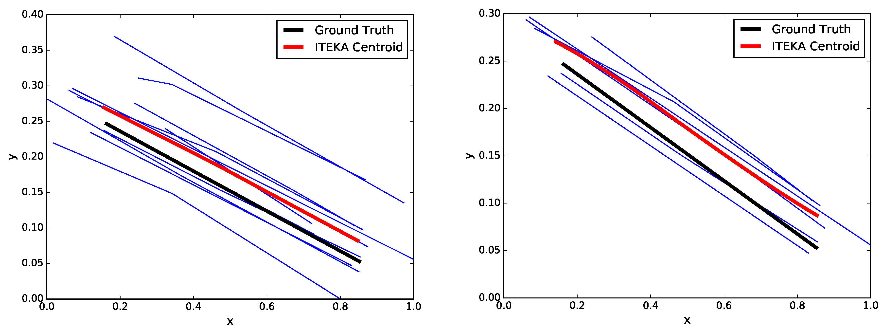
3.2. Averaging and Outliers Removal

The averaging is obtained using either medoid or centroid approaches, which corresponds to Steps 2 and 4 in Figure 1. When iTEKA centroid (Algorithm 1) is selected, the medoid according to the ${\mathcal{K}}_{\mathrm{rdtw}}$ measure is used to initiate the reference time series $C_0$.

Once the centroid C of set $\mathbf{X}$ is obtained, the mean ${\mu }_{C,\mathbf{X}}$, and the variance, ${\sigma }_{C,\mathbf{X}}$, of $Log\left({\mathcal{K}}_{\mathrm{rdtw}}(C,\mathbf{x})\right)$ measure are evaluated, as x samples the elements of X.

For iTEKA approach, when ${\sigma }_{C,\mathbf{X}}>\tau$, the time series $\mathbf{x}$ such that

$$Z_{score}\left(x\right)=\frac{Log\left({\mathcal{K}}_{\mathrm{rdtw}}(C,\mathbf{x})\right)-{\mu }_{C,\mathbf{X}}}{{\sigma }_{C,\mathbf{X}}}\ge 0$$

(12)

are removed from the set $\mathbf{X}$, as far as $\left|\mathbf{X}\right|\ge 3$. Here, $\tau$ is a threshold that we empirically set to 5. Basically, all trajectories that are “log-distant” of at least one standard deviation are removed if ${\sigma }_{C,\mathbf{X}}>5$, and are kept otherwise.

For all other methods, the $Log\left({\mathcal{K}}_{\mathrm{rdtw}}\right)$ is replaced by the similarity measure that is used instead. This corresponds to Step 3 of the procedure depicted in Figure 1.

Once the outliers have been removed from set $\mathbf{X}$, if any, a second averaging procedure is then carried out on the new set ${\mathbf{X}}^{\prime }$ initialized with the previous centroid estimation, $C_0=C$ (Step 4 in Figure 1). The final centroid estimation C associated to the initial set $\mathbf{X}$ of GPS trajectories is finally provided by the averaging procedure depicted in Figure 1.

Figure 5 gives an example of this outlier removal procedure used during Step 3. Note that this procedure does not guarantee that the centroid estimate would be closer to the ground truth. Sometimes, once the outlier removal has been applied, the centroid estimate worsens the assessment measure. However, at least on the training data, it brought on average some assessment measure improvement.

3.3. Post-Processing of the Centroid Estimate

The final step (Step 5 of the processing pipeline presented in Figure 1) consists in downsampling the centroid estimate C such that it contains the average number of samples that characterize the initial set of trajectories. This is achieved using a polygonal curve approximation procedure, as described in [24].

4. Experimentation

The experimentation was carried out using the training dataset provided by the Averaging GPS segments competition setup [14] at University of Eastern Finland (https://cs.uef.fi/sipu/segments/). It consisted in estimating a cleaned GPS trajectory segment given a set of GPS trajectories corresponding to the same segment. Only training data corresponding to a set of road segments were delivered along with ground truth trajectory for each considered road segments.

It is important to note that the assessment measure used to evaluate the competing approaches was not explicitly provided. However, on the training data, the challenge site makes it possible to obtain the average value of the assessment measure obtained by a given method by submitting the set of solution trajectories produced by this method. We show below that this unknown assessment measure used to rank the competing methods is not strongly correlated to a RMSE measure between an estimated trajectory and the corresponding ground truth trajectory. The assessment measure (as we learned once the challenge was closed) is referred to as HC-SIM, a hierarchical version of the C-SIM measures described in [2]. The C-SIM measure is based on the notion of grid which partition the 2D space in contiguous cells of 25 m${}^2$. To compare two trajectories, the Jaccard index was evaluated by performing the ratio of the common cells shared by the two trajectories with the union of the cells traversed by the two trajectories. To avoid the effect of the discretization of the grid, the trajectories were slightly dilated, which had the effect of enlarging a bit of the trajectories by adding some of the adjacent cells. The HC-SIM (H for hierarchical) measurement was derived from the C-SIM measure by varying the size of the cells and providing a weighted average as output. The details of this measure have not yet been published by the authors. However, as mentioned above, an evaluation program allowed producing the results presented below. The HC-SIM measure gives a percentage of similarity between two trajectories (hence, it varies in $[0,100\%]$).

We evaluated eight approaches: (i) four medoid based models, namely Euclidean, DTW, ${\mathcal{K}}_{\mathrm{rdtw}}$ and soft-DTW with medoid; and (ii) four centroid based models, namely Euclidean, DBA, soft-DTW and iTEKA centroid methods.

All approaches shares the T meta parameter, which defines the size of the resample trajectories. In addition, ${\mathcal{K}}_{\mathrm{rdtw}}$, iTEKA as well as the soft-DTW medoid and centroid methods require the set-up of two meta parameters, $\nu$ and $\gamma$, respectively, the bandwidth of the local kernel parameter (Equation (4)) and T, the length of the trajectories, once they have been resampled after the second preprocessing step.

For all methods, these meta parameters were varied for all training sets of trajectories simultaneously, such as maximizing the HC-SIM measure obtained by the centroid estimates.

We first selected $\nu$ and $\gamma$ in the discrete set {.1,. 5, 1, 2, 3, 4, 5, 6, 7, 8, 9, 10, 11, 12, 13, 14, 15, 16, 17, 18, 19, 20} while T value was selected within $\{100,200,300\}$.

According to Figure 6, the meta parameters $\nu$ and T are correlated for the iTEKA algorithm. On the training data, a simple grid search led to selecting $\nu =6$ and $T=200$, which allowed reaching a HC-SIM of $68.5\%$.

Similarly, according to Figure 7, the meta parameters $\gamma$ and T are correlated for the soft-DTW centroid. On the training data, a simple grid search led to selecting $\gamma =2$ and $T=100$, which allowed reaching a HC-SIM score of $67.39\%$.

Figure 6 and Figure 7 show that over-sampling has an important impact on the HC-SIM measure of the estimated centroids.

As stated above, the HC-SIM measure is not strongly correlated to the RMSE measure. The correlation between RMSE and HC-SIM measures when varying $\gamma$ parameter for soft-DTW or $\nu$ for iTEKA is, respectively, $-61\%$ and $+67\%$. This shows the difficulty of this challenge, since the ground truth provided on the training data does not directly help to train the models. Hence, selecting the minimum RMSE value would not lead to the best HC-SIM measure.

Table 1. Best HC-SIM (in %) obtained with or without outlier removal for the eight tested methods. The best obtained HC-SIM value are indicated in bold cases.

Method	Without Outlier Removal	With Proposed Outlier Removal
Euclidean Medoid [25]	60.90	60.49
DTW Medoid [26]	63.16	63.16
${\mathcal{K}}_{\mathrm{rdtw}}$ Medoid [23]	61.20	61.20
soft-DTW Medoid [9]	61.29	61.29
Euclidean Centroid [27]	67.28	67.54
DBA Centroid [28]	66.40	66.40
soft-DTW Centroid [9]	67.47	67.39
iTEKA Centroid [13]	68.21	68.28

synthesizes the results obtained by the eight tested methods. It turns out that centroid based methods are much more accurate than the medoid ones. The averaging scheme is thus quite important. One can notice that, on this benchmark characterized by small and simple trajectories, the Euclidean averaging performed quite well, reaching a 67.15% HC-SIM when outlier removal was considered. This is better than soft-DTW that obtained 66.93%. The best method on this benchmark is iTEKA that reached 67.63% HC-SIM with outlier removal.

However, with the absence of an analytical knowledge of the HC-SIM measure that is used, we cannot provide confidence intervals or state whether these results are significant or not.

The final results of the challenge (http://cs.uef.fi/sipu/segments/results.html), as provided by the organizers, are given in

Table 2. Challenge results as produced by the organizers: ranking of the competing methods according to the HC-SIM measure (in %). The iTEKA method corresponds to methods A and E.

Rank	Train	Test	Length	Points	Time
A	68.5%	62.2%	99%	9882%	30 min
B	67.1%	62.0%	99%	89%	seconds
C	70.4%	61.8%	101%	83%	seconds
D	68.0%	61.8%	99%	83%	seconds
E	68.3%	61.7%	99%	145%	30 min
F	66.6%	61.5%	100%	70%	seconds
G	67.4%	61.2%	100%	107%	10 min
H	66.6%	61.2%	102%	205%	seconds
I	68.1%	60.9%	99%	67%	seconds
DTW Medoid	57.3%	55.3%	98%	169%	1 h
CellNet	64.7%	61.2%	96.3%	144%	seconds

. When no post-processing was used, iTEKA method ranks first (Method A), but, as shown in the last two columns of the table, the method is slow and induces a spurious number of points in the averaged trajectory that is provided. When reducing the number of points of the centroid trajectory, using the down-sampling post-processing, the HC-SIM quality measure dropped, as shown for Method E that corresponds to the processing pipeline presented in Figure 1 when iTEKA was used. The slight differences in the results apparent in Table 1 and Table 2 are probably due to a slight change in the HC-SIM measure that produces differences in the selection of the meta parameters for the submitted results.

Finally, Figure 8 presents the elapsed time in a logarithmic scale when T increases (the length of the re-sampled trajectories) for the centroids approaches. The Euclidean centroid method is clearly the most efficient one, as expected, followed by the iTEKA method that is significantly faster than the soft-DTW centroid one. The least efficient method is clearly DBA. Indeed, although all the tested algorithms were run on the same architecture and operating system, the observed differences of processing efficiency may be due, at least partly, to difference in the implementation choices. The medoid-based methods are more costly since their dependence with the size of the set is quadratic, while it is linear for centroid-based methods.

5. Conclusions

We have described a procedure for cleaning noisy sets of GPS trajectories corresponding to road segments. This procedure includes, in the first stage, an oversampling of the trajectories, prior to the calculation of a centroid or the search for a medoid, which composes the second stage of the procedure. It also includes, as a third stage, the detection and suppression of potential outliers, which improves on average the HC-SIM measure for almost all centroid based methods. A down-sampling finalizes the procedure to produce centroid/medoid estimates whose lengths match the average length of the input trajectories.

The experiment allowed comparomg time elastic and Euclidean averaging approaches with more straightforward medoid approaches.

Our experimentation showed that: (i) centroid based methods outperform medoid based methods; (ii) the outlier detection and removal step improves on average the HC-SIM of final centroid estimation, but not the HC-SIM of the medoid selection; and (iii) over-sampling seems to also be a valuable step.

With the limited training data, it cannot be guaranteed that the comparative results presented here are effectively significant. However, it clearly emerged from our experimentation that centroid-based approaches outperform medoid-based approaches. Furthermore, the algorithmic complexity is clearly in favor to centroid-based approaches, since it is linear with the size of the sets of trajectories that are processed, whereas it is quadratic for medoid-based approaches.

As a perspective, to improve the HC-SIM quality of the cleaned trajectory estimation, one should consider the optimization of the meta parameters (T and $\tau$ essentially, as $\nu$ or $\gamma$ may be considered as a function of T) on each segment of road (instead on the whole set of segments), according to its topology. In that line of improvement, one should try first to clusterize the GPS datasets according to the segment shapes, and then optimize for each cluster the meta parameters.

References

1. Shi, W.; Shen, S.; Liu, Y. Automatic generation of road network map from massive GPS, vehicle trajectories. In Proceedings of the 2009 12th International IEEE Conference on Intelligent Transportation Systems, St. Louis, MO, USA, 4–7 October 2009; pp. 1–6. [Google Scholar] [CrossRef]
2. Mariescu-Istodor, R.; Fränti, P. Grid-Based Method for GPS Route Analysis for Retrieval. ACM Trans. Spat. Algorithms Syst. 2017, 3, 8:1–8:28. [Google Scholar] [CrossRef]
3. Mariescu-Istodor, R.; Fränti, P. CellNet: Inferring Road Networks from GPS Trajectories. ACM Trans. Spat. Algorithms Syst. 2018, 4, 8:1–8:22. [Google Scholar] [CrossRef]
4. Welch, G.; Bishop, G. An Introduction to the Kalman Filter; University of North Carolina at Chapel Hill: Chapel Hill, NC, USA, 1995. [Google Scholar]
5. Evensen, G.; van Leeuwen, P.J. An Ensemble Kalman Smoother for Nonlinear Dynamics. Mon. Weather Rev. 2000, 128, 1852–1867. [Google Scholar] [CrossRef] [Green Version]
6. Panangadan, A.V.; Talukder, A. A variant of particle filtering using historic datasets for tracking complex geospatial phenomena. In Proceedings of the 18th ACM SIGSPATIAL International Symposium on Advances in Geographic Information Systems, ACM-GIS, San Jose, CA, USA, 3–5 November 2010; pp. 232–239. [Google Scholar] [CrossRef]
7. Velichko, V.M.; Zagoruyko, N.G. Automatic Recognition of 200 Words. Int. J. Man-Mach. Stud. 1970, 2, 223–234. [Google Scholar] [CrossRef]
8. Sakoe, H.; Chiba, S. A dynamic programming approach to continuous speech recognition. In Proceedings of the 7th International Congress of Acoustic, Budapest, Hungary, 18–26 August 1971; pp. 65–68. [Google Scholar]
9. Cuturi, M.; Blondel, M. Soft-DTW: A Differentiable Loss Function for Time-Series. In Proceedings of the 34th International Conference on Machine Learning, Sydney, Australia, 6–11 August 2017; Precup, D., Teh, Y.W., Eds.; International Convention Centre: Sydney, Australia, 2017; Volume 70, pp. 894–903. [Google Scholar]
10. Marteau, P.F.; Gibet, S. On Recursive Edit Distance Kernels with Application to Time Series Classification. IEEE Trans. Neural Netw. Learn. Syst. 2014, 26, 1121–1133. [Google Scholar] [CrossRef] [PubMed]
11. Hausner, M. A Vector Space Approach to Geometry; Dover Publications Inc.: Mineola, NY, USA, first edition 1965, second edition 1998.
12. Petitjean, F.; Forestier, G.; Webb, G.; Nicholson, A.; Chen, Y.; Keogh, E. Dynamic Time Warping Averaging of Time Series Allows Faster and More Accurate Classification. In Proceedings of the 14th IEEE International Conference on Data Mining, Shenzhen, China, 14–17 December 2014; pp. 470–479. [Google Scholar]
13. Marteau, P.F. Times series averaging and denoising from a probabilistic perspective on time-elastic kernels. Int. J. Appl. Math. Comput. Sci. 2019, 29, 375–392. [Google Scholar]
14. Fränti, P.; Mariescu-Istodor, R. Averaging GPS segments challenge 2019. unpublished work. 2019. [Google Scholar]
15. Bahlmann, C.; Haasdonk, B.; Burkhardt, H. On-Line Handwriting Recognition with Support Vector Machines A Kernel Approach. In Proceedings of the Eighth International Workshop on Frontiers in Handwriting Recognition (IWFHR’02), Niagara on the Lake, ON, Canada, 6–8 August 2002; IEEE Computer Society: Washington, DC, USA, 2002; p. 49. [Google Scholar]
16. Shimodaira, H.; Noma, K.i.; Nakai, M.; Sagayama, S. Dynamic Time-alignment Kernel in Support Vector Machine. In Proceedings of the 14th International Conference on Neural Information Processing Systems: Natural and Synthetic, Vancouver, BC, Canada, 3–8 December 2001; MIT Press: Cambridge, MA, USA, 2001; pp. 921–928. [Google Scholar]
17. Cuturi, M.; Vert, J.P.; Birkenes, O.; Matsui, T. A Kernel for Time Series Based on Global Alignments. In Proceedings of the 2007 IEEE International Conference on Acoustics, Speech and Signal Processing–ICASSP ’07, Honolulu, HI, USA, 15–20 April 2007; pp. 413–416. [Google Scholar] [CrossRef]
18. Fasman, K.H.; L., S.S. An introduction to biological sequence analysis. In Computational Methods in Molecular Biology; Salzberg, S.L., Searls, D.B., Kasif, S., Eds.; Elsevier: Amsterdam, The Netherlands, 1998; pp. 21–42. [Google Scholar]
19. Wang, L.; Jiang, T. On the Complexity of Multiple Sequence Alignment. J. Comput. Biol. 1994, 1, 337–348. [Google Scholar] [CrossRef] [PubMed] [Green Version]
20. Just, W.; Just, W. Computational Complexity Of Multiple Sequence Alignment With Sp-Score. J. Comput. Biol. 1999, 8, 615–623. [Google Scholar] [CrossRef] [PubMed]
21. Hautamaki, V.; Nykanen, P.; Franti, P. Time-series clustering by approximate prototypes. In Proceedings of the 2008 19th International Conference on Pattern Recognition, Tampa, FL, USA, 8–11 December 2008; pp. 1–4. [Google Scholar] [CrossRef]
22. Petitjean, F.; Ketterlin, A.; Gançarski, P. A Global Averaging Method for Dynamic Time Warping, with Applications to Clustering. Pattern Recogn. 2011, 44, 678–693. [Google Scholar] [CrossRef]
23. Marteau, P. Times series averaging from a probabilistic interpretation of time-elastic kernel. arXiv 2015, arXiv:1505.06897. [Google Scholar]
24. Marteau, P.; Ménier, G. Speeding up simplification of polygonal curves using nested approximations. Pattern Anal. Appl. 2009, 12, 367–375. [Google Scholar] [CrossRef]
25. Newling, J.; Fleuret, F. A Sub-Quadratic Exact Medoid Algorithm. In Proceedings of the International Conference on Artificial Intelligence and Statistics (AISTATS), Fort Lauderdale, FL, USA, 20–22 April 2017; pp. 185–193. [Google Scholar]
26. Annam, J.R.; Mittapalli, S.S.; Bapi, R.S. Time series Clustering and Analysis of ECG heart-beats using Dynamic Time Warping. In Proceedings of the 2011 Annual IEEE India Conference, Hyderabad, India, 16–18 December 2011; pp. 1–3. [Google Scholar] [CrossRef]
27. Liberti, L.; Lavor, C.; Maculan, N.; Mucherino, A. Euclidean Distance Geometry and Applications. SIAM Rev. 2014, 56, 3–69. [Google Scholar] [CrossRef]
28. Petitjean, F.; Gançarski, P. Summarizing a set of time series by averaging: From Steiner sequence to compact multiple alignment. J. Theor. Comput. Sci. 2012, 414, 76–91. [Google Scholar] [CrossRef] [Green Version]
Figure 1. Processing pipeline overview: The meta parameters ν (iTEKA averaging method) and γ (soft-DTW averaging method) are defined, respectively, in Equations (5) and (8). The T meta parameter is the length of the trajectories when they have been over-resampled during the pre-processing step and is defined in Section 3.1. The τ parameter is a threshold involved to decide whether a trajectory is an outlier and is defined in Section 3.2.
Applsci 09 02736 g001
Figure 2. Three possible alignments path (green, red, black) between time series x and x .
Applsci 09 02736 g002
Figure 3. The forward (left) and backward (right) alignment kernel matrices.
Applsci 09 02736 g003
Figure 4. The forward–backward alignment kernel matrix.
Applsci 09 02736 g004
Figure 5. iTEKA centroid estimate (in red) before pruning (left) and after pruning (right). The blue lines represent trained data, i.e. measured GPS trajectories corresponding to a street segment. The x,y coordinates are latitude and longitude converted in UTM coordinates then normalized in [ 0 ; 1 ] .
Applsci 09 02736 g005
Figure 6. HC-SIM (in %) of the iTEKA centroid estimate relative to the ground truth trajectory when ν varies for T = 50 , T = 100 , 200 and 300.
Applsci 09 02736 g006
Figure 7. HC-SIM (in %) of the soft-DTW centroid estimate relative to the ground truth trajectory when γ varies for T = 50 , 100, 200 and 300.
Applsci 09 02736 g007
Figure 8. Elapsed processing time as the size of the re-sampled trajectories, T, varies ( T { 50 , 100 , 200 , 300 } ).
Applsci 09 02736 g008