Article

Turbocharger Axial Turbines for High Transient Response, Part 2: Genetic Algorithm Development for Axial Turbine Optimisation

Department of Mechanical and Aerospace Engineering, Brunel University, London UB8 3PH, UK
*
Author to whom correspondence should be addressed.
Appl. Sci. 2019, 9(13), 2679; https://doi.org/10.3390/app9132679
Submission received: 29 April 2019 / Revised: 20 June 2019 / Accepted: 25 June 2019 / Published: 30 June 2019

Abstract

:
In a previous paper, a preliminary design methodology was proposed for the design of an axial turbine, replacing a conventional radial turbine used in automotive turbochargers, to achieve improved transient response, due to the intrinsically lower moment of inertia. In this second part of the work, the focus is on the optimisation of this preliminary design to improve on the axial turbine efficiency using a genetic algorithm in order to make the axial turbine a more viable proposition for turbocharger turbine application. The implementation of multidisciplinary design optimisation is essential to the aerodynamic shape optimisation of turbocharger turbines, as changes in blade geometry lead to variations in both structural and aerodynamics performance. Due to the necessity to have multiple design objectives and a significant number of variables, genetic algorithms seem to offer significant advantages. However, large generation sizes and simulation run times could result in extensively long periods of time for the optimisation to be completed. This paper proposes a dimensioning of a multi-objective genetic algorithm, to improve on a preliminary blade design in a reasonable amount of time. The results achieved a significant improvement on safety factor of both blades whilst increasing the overall efficiency by 2.55%. This was achieved by testing a total of 399 configurations in just over 4 h using a cluster network, which equated to 2.73 days using a single computer.

1. Introduction

This work is a continuation of a previous paper, presenting a preliminary design methodology for axial turbocharger turbines [1]. The computational resource increment in recent years has allowed multidisciplinary design optimisation (MDO) to permeate multiple R&D disciplines, to the point of becoming essential in aerodynamic shapes optimization [2,3]. Traditionally, the design process required a high degree of engineering involvement and was reliant on designer experience in the field. Over the past 20 years, with the improvement in computational resources and in fluid dynamics algorithms accuracy, the trend in research has shifted to a predominantly numerical approach: “In regard to human interface, MDO developers and users seem to have arrived at a consensus that computer-based MDO methodology is an increasingly useful aid to the creative power of human mind” [4].
In the specific case of turbines, a multidisciplinary approach is necessary as changes in blade geometry lead to variations in both structural and aerodynamics results, rendering it impossible to obtain realistic geometries without taking both fields into consideration.
Design optimisation processes are largely portable across similar applications, thus research can be conducted on optimisation techniques in axial turbines for different applications. Multiple sources are present, however, it is clear that the design optimisation topic is highly sensitive to manufacturers, with the majority of the sources being obsolete [5,6], as highlighted by the most recent paper on the topic [7]. The most notable common trait in previous examples of design optimisation is the fact that most of them were carried out using genetic algorithms (GAs). The method is one of the most popular in MDO, as it can handle “discontinuities, multimodality, disjoint feasible spaces and noisy function evaluations” [8], which are common features in the optimisation task to be carried out, as most of the objectives are effectively described by discontinuous functions. These capabilities are what distinguish GAs from its competitors.
In recent years, research on this relatively new topic has been extremely prolific, with numerous innovations and schools of thoughts developing at an incredible pace. In 2018 alone, more than 20,000 papers or books have been published on the topic of genetic algorithm optimisation [9]. The general consensus gauged from surveys [10,11] is that methodologies and implementations are still in an embryonal stage, and that there is no clear best implementation of the method. The authors’ conclusions are that techniques should be evaluated in a case-by-case manner.
Recent literature focuses on theoretical of purely numerical approaches, especially in a manufactural design optimisation task. The complexity and time-consuming nature of MDOs featuring multiple evaluations, however, is preventing any complete (i.e., from preliminary to final) design optimisation tasks relevant for this project. Research has followed two different approaches, either reducing the objectives to optimise for [12], or accepting less accurate results by utilising simpler mathematical models [13].
The first example of axial turbine parameter optimisation available was published in 1985 [5]. The algorithm, coded in FORTRAN, allowed the user to obtain a preliminary blade design with 11 independent parameters, mathematically derived by the author. The other 14 parameters were optimised by using a mathematical model. While the results were heavily approximated, this publication is of absolute importance from an historic point of view, as Pritchard, in their ingenuity, understood the need of a parametric blade generation to allow a faster preliminary design process, thus allowing engineers to apply their experience and expertise in a focussed way. The procedure features numerous approximations and essentially no integration with computational fluid dynamics (CFD), however it should be noted that the algorithm was executed on a computer with 8 kB of RAM [14].
A systematic automatic design optimisation approach for turbine blades was firstly developed in 1996 [15] and was confirmed to be effective in 1997 [16]. The authors considered a GA approach to be possible, however overly expensive in terms of computational resources. In 1999, the first GA approach was implemented, and the authors utilised a simplified mathematical model, which estimated profile losses through a two-dimensional approximated CFD analysis [6]. The algorithm yielded extremely promising results, with two-dimensional losses reduced by an order of magnitude compared to baseline blades. The optimisation task was proved to be an effective tool for design exploration, as it aided the visualisation of trends and general behaviour with varying parameters. The innovation allowed blade designers to focus on the three-dimensional aspect of the design process, as they were provided with an excellent baseline.
Öksüz and Akmandor published their MDO using a GA approach on an axial turbine in 2010 [7]. The authors optimised an axial turbine and stator profiles to maximise efficiency and torque. Once again, the main challenge was the incredible amount of computational resources needed to perform multiple CFD evaluations. Their 37 parameters GA implementation used an approximation exploit, which featured a surrogate model, with a dynamic correction factor calculated as a function of the percentage difference between a fast, inaccurate CFD analysis, and a high-fidelity one. Algorithm run times required to implement this solution were relatively small if compared to a traditional design optimisation task, with 20 days of CPU usage for the first 10 generations. This process was also carried out with no consideration for any structural element, thus once again providing results only useful in a preliminary design environment. The implementation showed that MDO using GAs is not only beneficial, but also highly viable.
Across all reviewed literature, conclusions tend to be coherent in suggesting the methodology to be extremely promising, with computational time being the limiting factor preventing a widespread application. Computational resources have drastically increased since the last publication, however they still are not at a level that would allow a pure genetic algorithm to be implemented. Thus, any GA implementation involving CFD analysis should focus on minimising algorithm run time. The techniques used in this article are analysed in the next section.

2. Genetic Algorithm Dimensioning

An automated MATLAB script (R2018a, MathWorks, Natick, MA, USA) was set to generate a population, simulate the members in a complex ANSYS Workbench project (18.2, ANSYS Inc., Canonsburg, PA, USA), and evaluate the results through a fitness function. The foundation of the coding methodology was to allow multiple similar problems to be solved by the same script with minimal adjustments. This decision dramatically increased the complexity of the code, forcing an object-oriented programming approach [17].
The main aim of the implementation was to provide a fast, reliable, and effective tool for design optimisation of axial turbines or other similar problems, thus many features of this GA are geared towards convergence rate and speed of execution, rather than focusing on providing the absolute optimal result.

2.1. Population Member Chromosome Encoding

Randomly generated chromosomes needed to be encoded in binary form, to facilitate crossover, population, and mutation calculations. It can also help assess the quality of the design optimisation approach, by giving a total design space dimension. Each of the 48 parameters was encoded as a bit sequence of length proportionate to the perceived relevance in the design quality. Once the value ranges were defined, parameters then had 2 x number of possible values, ranging from minimum to maximum, with x being the number of assigned bits to that value. The total number of bits is essential to estimate a correct number of population members, and it was chosen to be the maximum possible for a realistic execution. Number of bits allocation is discussed in the following section.

2.2. Population Size

The available literature in genetic algorithm dimensioning is surprisingly shallow, as researchers seem to have focused on more efficient procedures and direct applications, more than studying the actual dimensioning of the GA parameters. It should be noted that applications such as the one presented in this article, which feature significantly longer (time-wise) design evaluation phases relative to data processing phases are not a common occurrence. The dimensioning of this algorithm was derived from a statistical analysis of a generic GA, with several corrections applied to account for out-of-ordinary implemented methodologies [18]. Population number is constrained in the following way:
N i , 1 2 > 2 N b ,
N i , 2 = log 2 [ 1 ( 1 p m i s s ) 1 N b ] ,
N i = M a x ( N i , 1   ; N i , 2 ) ,
where N i   is the population number, N b is the bit size of every chromosome, p m i s s is the probability of a bit having the same value throughout the genetic pool. p m i s s was chosen to be 1 / 1024 as suggested by the literature [18]. This value was found to be appropriate for medium size GAs as this one through testing. Values of population numbers against total bits are shown as a continuous function in Figure 1.
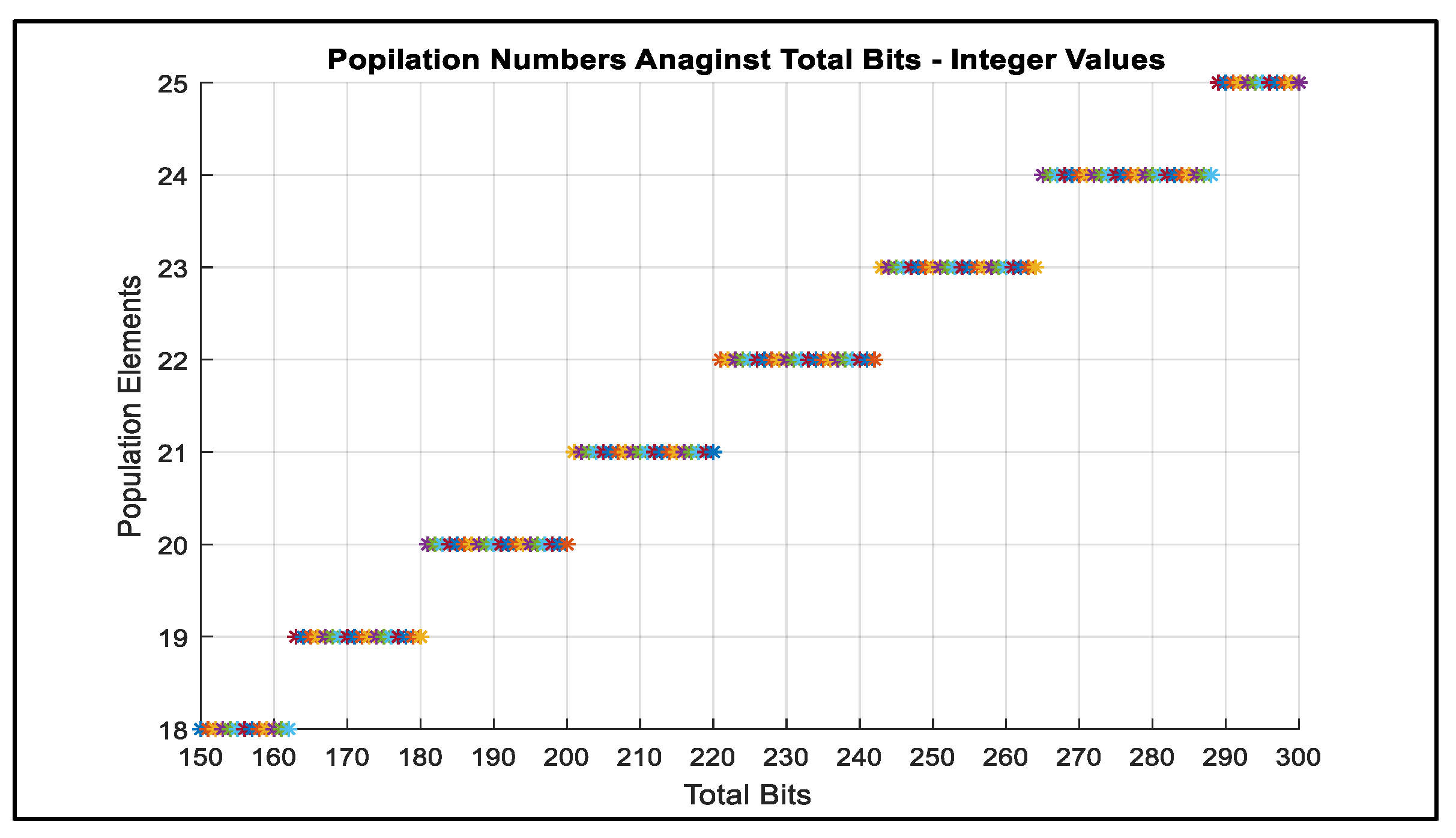
Due to technical limitations, the maximum population number was set to be 21. This was chosen due to the implementation of a cluster network briefly explained in a Section 3.3, which was constrained by the number of computing facilities available. Another plot was then produced (Figure 2) using only integer values of population sizes, resulting in the chosen number of bits per chromosome to be 220.

2.3. Mutation Rate

Gutowski suggested multiple formulations to optimally determine the mutation rate of a GA. Mutation is fundamental in a GA as it increases the coverage of the design space. Gutowski suggests multiple equations to be used to calculate mutation rates, shown below:
P m u t M a x = 1 2 1 N b ,
P m u t M i n = 1 ( N i 1 N i ) 1 N b ,
P m u t n a t 1 0.82 1 N b ,
where P m u t M a x , P m u t M i n , and P m u t n a t being the maximum, minimum, and suggested mutation rate for every bit for the algorithm at each iteration. The minimum mutation rate is calculated assuming an average of one chromosome mutating at each generation. The maximum mutation rate is set as the minimum required to have half the bits mutating at each generation. The suggested value is somewhat in-between the extremes and is defined as the maximum mutation probability that features negligible chances of two mutated chromosomes to perform a crossover with each other.
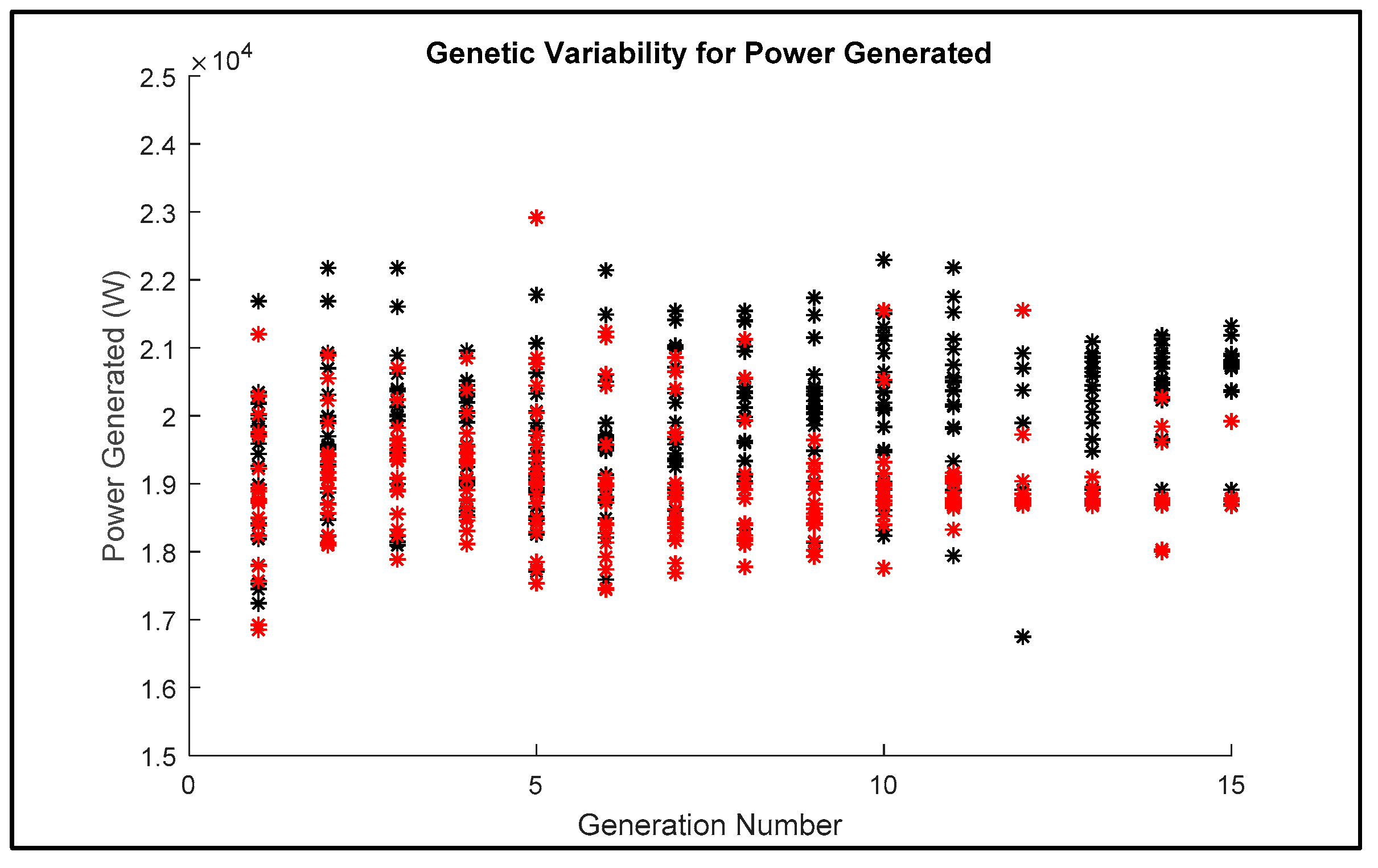
While this approach is the purely theoretical optimum, it was not practically viable. It served more as a valid guideline. More recent literature [19] showed that algorithm performance is not sensitive to mutation rate in terms of quality of results, however lower mutation rates achieve faster convergences. Literature also suggests a chromosome-based mutation rate, with complete regeneration in case of mutation, with one full reset per generation. The mutation rate in this case that would correspond to this value is 4.76%. Later analysis on GAs featuring Elitism (see Section 2.5) identified a low genetic variability, requiring a higher mutation rate. Figure 3 provides a visualisation of increased genetic variance in the population with increased mutation rate. Red data points are relative to the first 15 generations of the GA, run with 4.76% entire-bit mutation rate ( p m u t ) . Black data points are representative of the final results, run with a value for mutation probability of 15.10%. Generation 13 onwards show a complete convergence for low mutation rates, and the algorithm is essentially relying on a mutation to improve on fitness values, thus operating as an incredibly inefficient Monte-Carlo-style search. Mutation was also chosen to not affect the elite member, as to not lose any GA progress to chance. This approach prevented the process from being chaotic, thus higher variance was effectively positive. The metric for genetic variability was chosen to be power generated, as it was a secondary objective of the optimization. Results would still be influenced by this parameter, while not as heavily as efficiency. This gave the algorithm the ability to pursue the lowest energy path to the optimal power generated value, which was reached after 13 generations. In other words, a low mutation rate meant that essentially all turbines were generating the same amount of power after an extremely low amount of design space exploration, and that was determined by the elite member’s power generation value, which in turn was determined by the random initialization. By observing Figure 3, one can see the gradual reduction of variance around the elite members for every generation (at around 1.81 kW).

2.4. Generation Number

The minimum number of generations to be run is suggested by Gutowski for a statistically optimal solution [18]:
N g e n = l o g 10 ( N b ) l o g 10 ( 1 P m u t ) .
The theoretical number is unfeasibly high in a real-world scenario; thus the generation number should be as high as possible, up to the time limit allowed. An estimated minimum can be achieved by using values of p m u t instead. The resultant minimum generation number for this case was set at 16. This number, while seemingly small, was found to be rather correct in empirical tests, effectively due to elitism and parent selection choices. The final GA was run with 19 generations, and the GA would have had minimal improvement in maximum fitness if it were to be run for higher numbers of generations. Once again, the configuration surely is highly unlikely to converge to an absolute optimum, and tasks that would require an absolute optimum would require a substantially different layout in order to obtain it.

2.5. Elitism

Single-member elitism was implemented in this algorithm in order to ensure time efficiency of the script. By maintaining the best performing member of each generation, the algorithm is prevented from losing the best solution. This allows the algorithm to never lose progress, allowing for more flexibility in the search [20]. This technique is widely recognised as highly beneficial and is essential in the application discussed in this article, as any amount of computational resources invested in the optimisation had to yield positive or null results.

2.6. Crossover Method

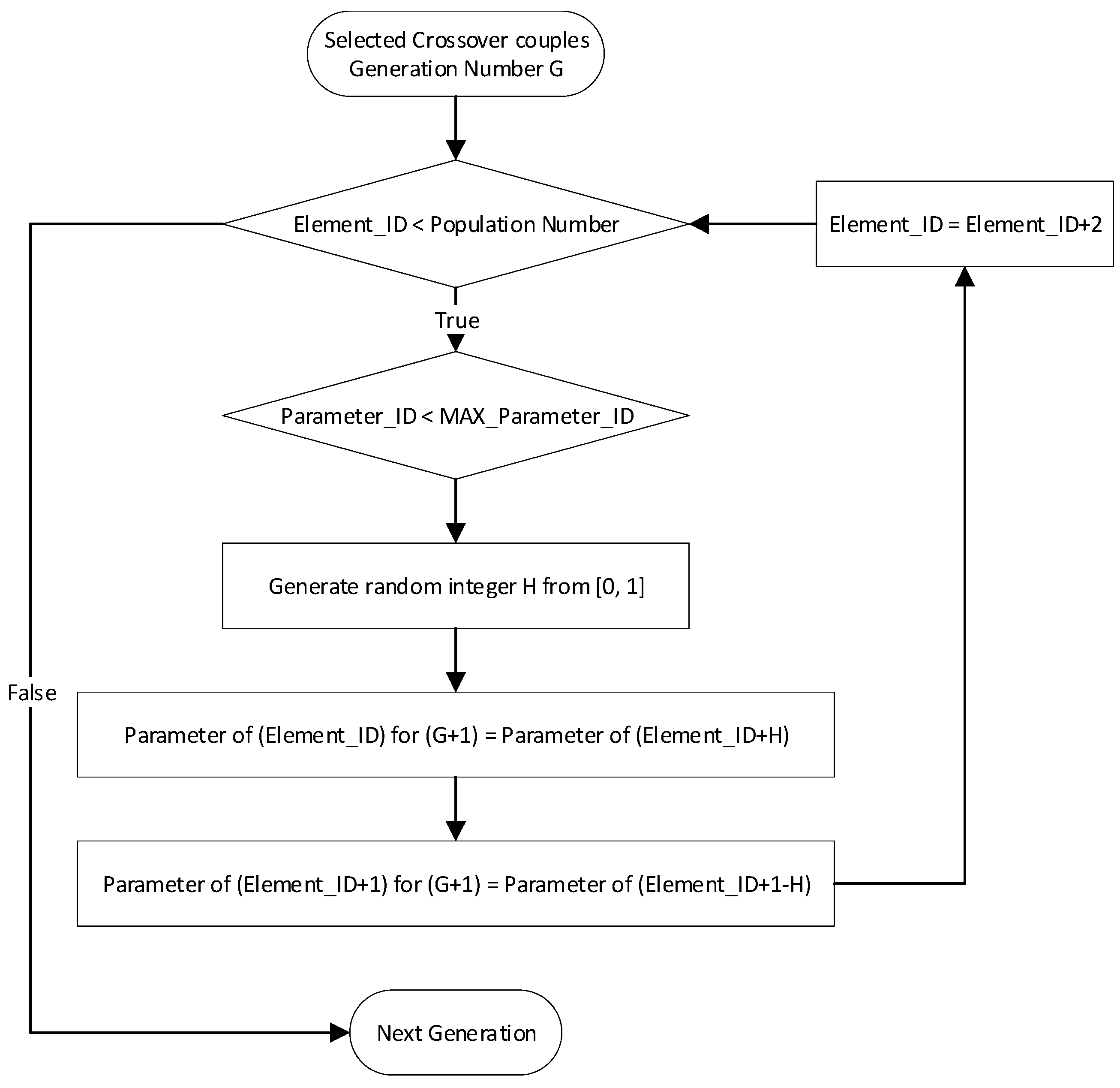
A uniform crossover method was chosen as this method is more exploratory when compared to alternative methods, like chromosome splitting. The crossover probability was set to a fixed 0.5 as default in uniform crossover methods, as no discontinuous parameter behaviour was observed in preliminary analysis [21]. Crossover chance, or the probability for a pair of mating chromosomes to effectively perform crossover, was set to 1 as it is recognised as inefficient and extremely uninfluential [19]. An overview of the method is detailed in Figure 4.

2.7. Parent Selection

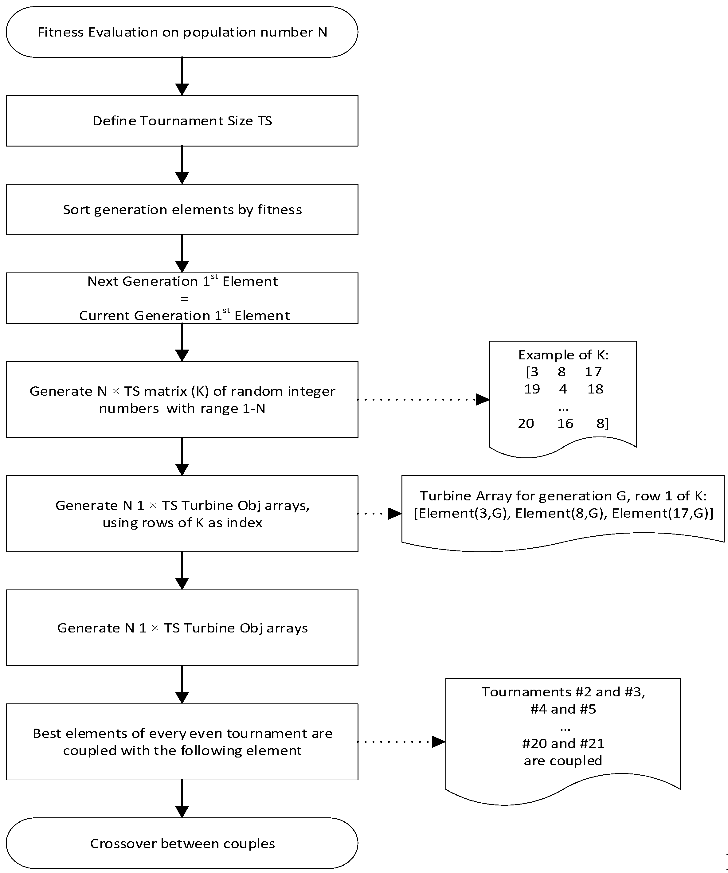
The chosen parent selection method was tournament mode with a size of 3. Compared to the alternative prominent parent selection method (roulette wheel selection), tournament selection does not feature stochastic noise [22]. Furthermore, it has been shown to be independent of the scaling of the algorithm fitness function [19]. The selection method with elitism schematic is shown in Figure 5.
Takeover time (τ) is defined as the number of generations “for the population to be filled with the best solutions found in the initial generation, in the absence of recombination and mutation” [19]. Lower takeover times lead to faster convergence, with higher chances of premature (i.e., local minimum) convergences. According to literature [19], the takeover time can be approximated using the equation:
τ   = 1 l n ( T s )   ( l n ( N i )   +   l n ( l n ( N i ) ) )   ,
where T s is the chosen tournament size. The result for this particular case presented in the example of Figure 6 (population size 21) was ~ 6 . This was an excessively low number, if the aim of the algorithm was to find the absolute optimal solution. However, this approach tries to find a better solution in a short time span, thus a premature convergence is effectively desired. Takeover time was found to be the most effective way of gauging the expected behaviour of a particular GA dimensioning, and values ranging from 5.5 to 7 were found to conform to the problem specific of a fast convergence, high average fitness gain per generation.

2.8. Fitness Function

The design constraints for this specific problem are presented in Table 1. Note the safety factor is defined as the ratio of Von Mises stress and the elastic limit of the material at 0.2% elongation.
To implement these design constraints the following fitness function was used shown in Table 1. The initial fitness function features efficiency maximisation exclusively, with the rest of the parameters being expressed as constraints:
F = 100   ×   η   ×   N + η ,
where F is the fitness value, η is the turbine efficiency, and N is a constraints check value of 0 if any values are outside acceptable ranges, 1 if within. The genetic pool in this configuration would, however, be strictly dependent on efficiency alone. This meant that the GA would not evolve towards a better blade overall, but towards a more efficient design exclusively. After numerous considerations and tests, a coefficient to account for power produced was added to the function. The reason behind this decision is that a turbine that would affect the flow in a more profitable way would not necessarily feature the maximum efficiency. Extremely, an exemplar A that would produce twice as much power, with 1% less efficiency compared to exemplar B would be considered closer to the optimum. Therefore, following some preliminary testing of the algorithm it was decided that an efficiency/power balance of 1% every ~2 kW (2060 W). In practical terms, a 77% efficiency, 17 kW power turbine worse than a 75%, 21.5 kW one. While the main task was to obtain a hyper efficient blade, results would not have been realistically better than the results obtained. The fitness function implemented in the final GA run was as following:
F = 100   ×   η   ×   N + 3   ×   η + ( W · 19000 ) / 2000 .
The scalar factors were added in to direct the genetic pool towards high fitness levels in case of populations featuring many failing chromosomes. The efficiency/power compromise ratio was revealed to be dramatically less impactful than the effective presence of the power factor, and in future applications this value should be tuned to fit the particular problem specifics.

3. Numerical Modelling Setup

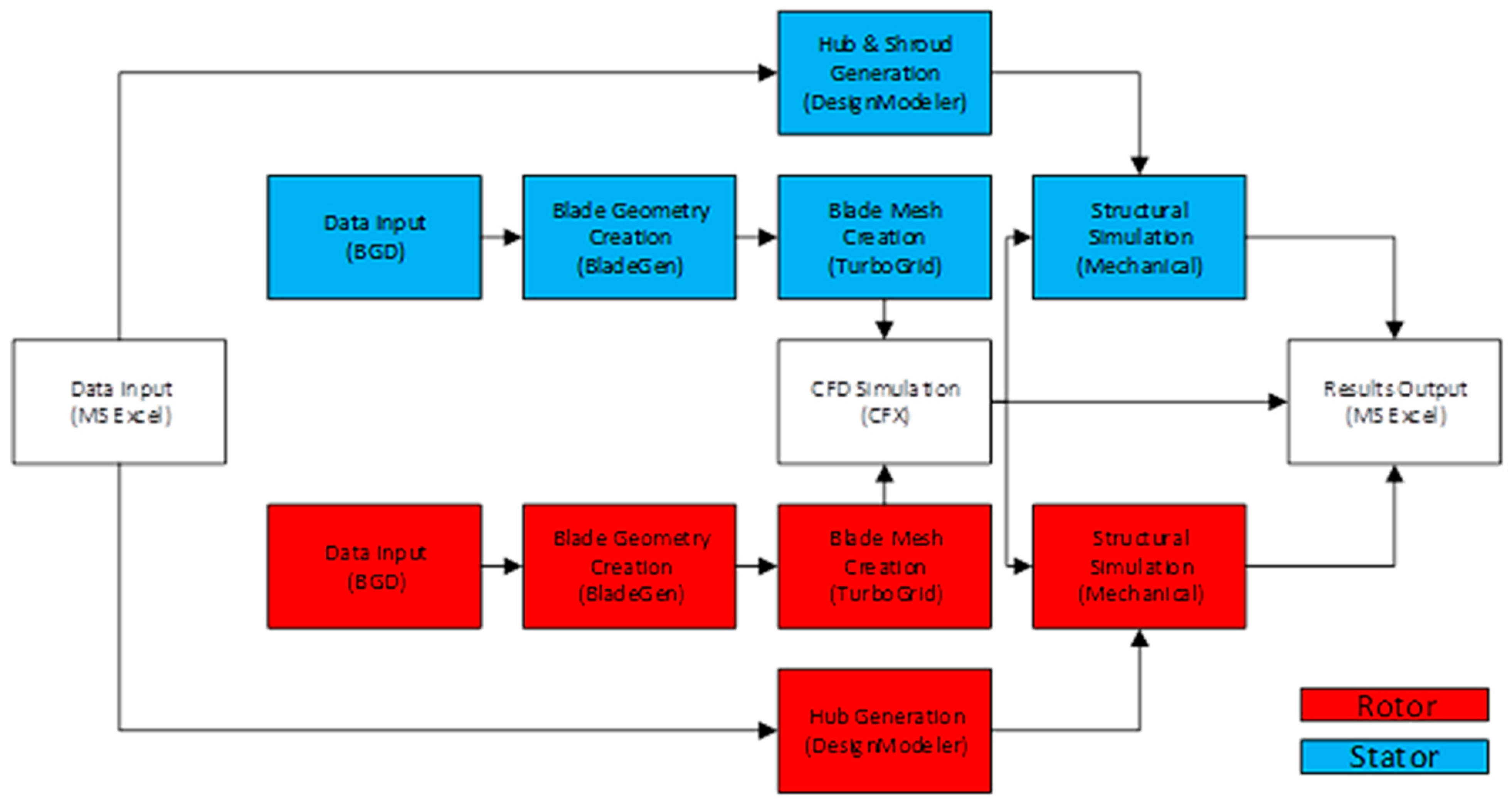
The numerical modelling was conducted using various applications from ANSYS Workbench 18.2 and schematic of the system is shown below in Figure 6 Within the file, the following applications are used:
  • Excel—Data interface tool between MATLAB and ANSYS Workbench;
  • BladeGen—Blade 3D geometry creation;
  • TurboGrid—Generation of blade meshes for CFD analysis;
  • CFX—Fluid analysis;
  • Mechanical—Structural analysis.

3.1. Computational Fluid Dynamics (CFD)

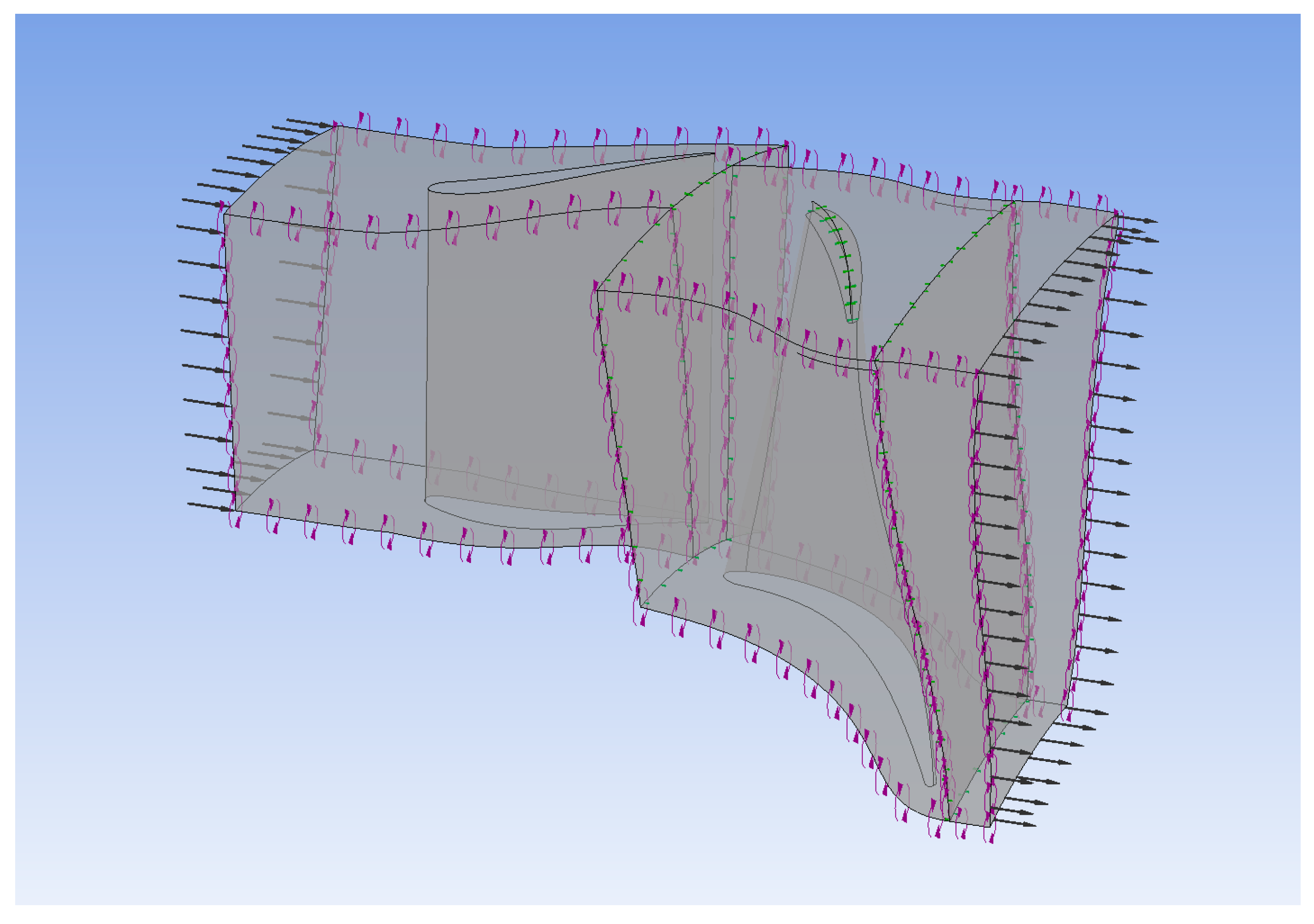
The CFD setup was conducted as explained in Part 1, based around the preliminary blade design [1]. The CFD was conducted using ANSYS CFX (18.2, ANSYS Inc., Canonsburg, Pa, USA) with the built in turbo mode. A 3-D overview of the CFD setup is shown below in Figure 7. The scalar values of the boundary conditions used for the simulation are shown below in Table 2.
  • The fluid is modelled as air (ideal gas).
  • K-ω shear stress transport turbulence model was chosen, which uses an automatic wall function, which automatically switches between a wall function and low-Re wall treatment.
  • Interfaces between stator and rotor, and rotor and outlet are selected as stage (mixing-plane).
  • Interfaces between stator blades and interfaces between rotor blades are set as periodic.
  • The meshes were setup using ANSYS Turbo Grid consisting of a total of 267,089 nodes. From previous investigation, this was found to be acceptable for accuracy.
  • Stator blade average Y + 12.2053.
  • Rotor blade average Y + 9.8685.

3.2. Finite Element Analysis (FEA)

The FEA setup was conducted using ANSYS Mechanical (18.2, ANSYS Inc., Canonsburg, PA, USA) with the material used for the analysis as Inconel 738 an overview of the boundary conditions is shown in with the specific boundaries highlighted Figure 8.
  • Temperature dependent properties were implemented into the material model using manufacturing data [23].
  • The fluid solid interaction (C) was added to the boundary conditions of each FEA model, importing temperature and pressures across the surface of the blades as calculated by the CFD simulation under design point boundary conditions.
  • Both blades were given the cylindrical support (B) applied to the bottom surface of the hub as shown below. The stator was fixed in the tangential direction, the rotor was fixed in the radial and axial directions.
  • A rotational velocity of 16,635 rad/s was applied to the rotor (A)
  • A displacement boundary (A) condition of 0 mm in the z direction was applied to the front surface of the stator hub to simulate a connection to the volute.
  • The rotor analysis was simulated using the Coriolis effect.

3.3. Algorithm Computational Cost

Each design evaluation cycle required an average of 11 min and 42 s, with specific times presented in Table 3. The relatively fast design evaluation was achievable through a simplification of the fluid-structure interface (FSI) modules on the Workbench project by directly importing the steady state CFD results. The average times resulted in an expected algorithm runtime of ~ 65 h and 31 min, or 2.73 days. The calculated runtime was highly theoretical and was subject to computer facility specific technicality problems.
In order to further improve run time of the algorithm, a cluster network was implemented, this solution cut the total running time down to little over 4 h. The solution consisted of a “master” computer, which would manage the data structure and all specific operations required to complete a genetic algorithm, and 21 “slave” computers, one for each population member, that were only tasked to perform simulations. The master PC would generate data sets and save them in a folder, shared across all computers.

4. Results and Discussion

As Table 4 shows, the optimisation process allowed a 2.55% gain in efficiency, which was the main aim of the fitness function; Safety factors defined as per Section 3.3 and calculated within ANSYS 18.2 Mechanical, shifted from an unacceptable range to being amply within design constraints; finally, turbine power output was decreased by a 1.51 kW. The CFD calculated power was, in fact, underestimated. Boundary conditions (mass flow rate at inlet, static pressure at outlet) were unfavourable as correlated to a significantly lower efficiency blade for high fitness blades. The high static pressure at the outlet entailed a discrepancy between high efficiencies blades, which would have produced lower static pressures at outlet, and generated power, as they did not produce maximum power at the specified boundary conditions.

4.1. Algorithm Design Exploration

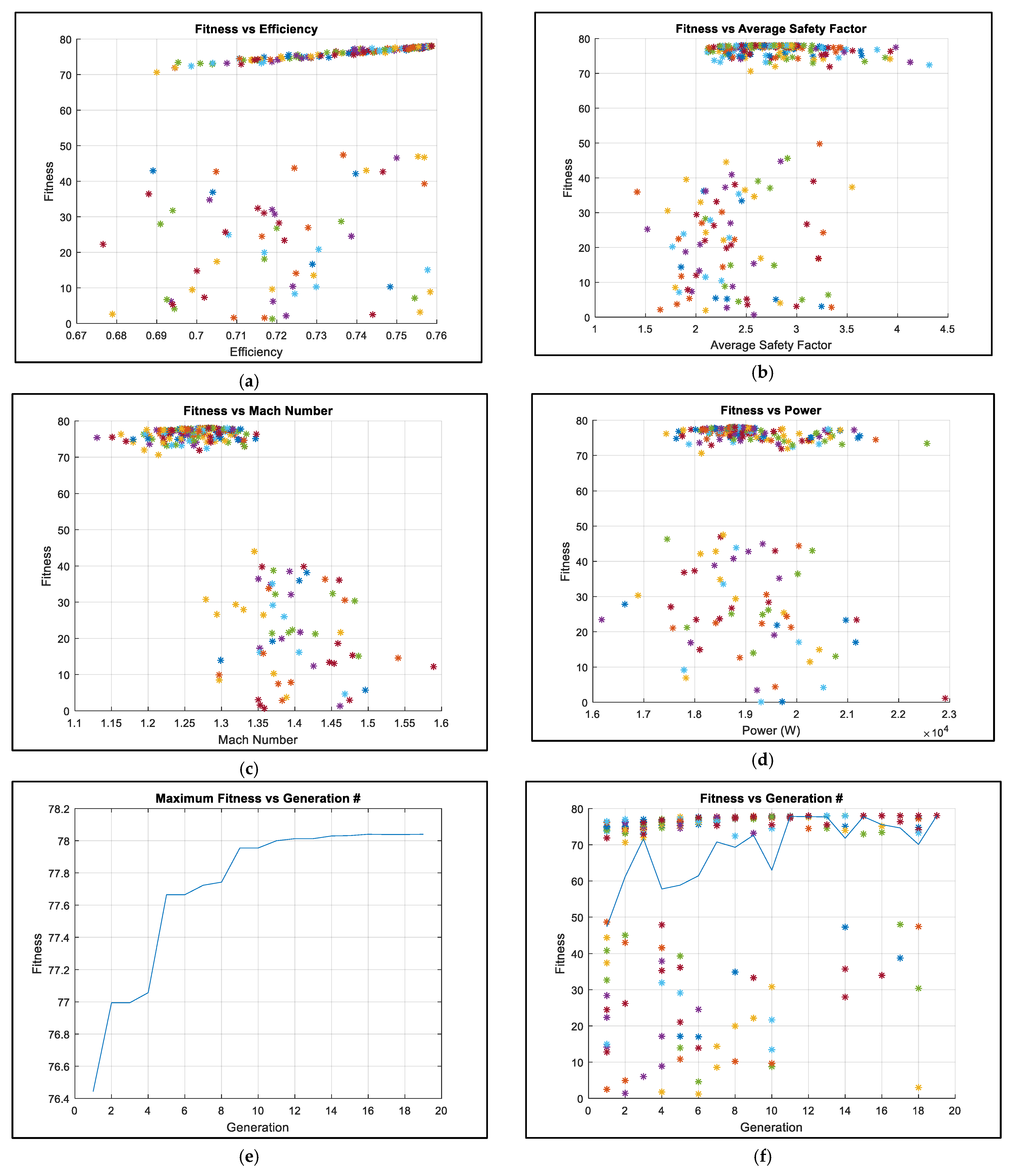
Figure 9 indicates the optimisation design exploration. The fitness values were plotted against optimisation objectives to show the influence of these parameters on design quality.
Figure 9a shows fitness against turbine efficiency across all design evaluations. An expected linear behaviour pattern is clearly recognisable, as the parameter acts as the main influence. Compared to the total number of design evaluations, an extremely low percentage of random and pseudo-random blades were created with efficiencies below 0.7. The results are encouraging in terms of design process evaluation, as one could conclude that a close to ideal starting point and ranges where selected. Failing elements majority falls between 0.72 and 0.74 efficiency. While it is hard to speculate on such information, the higher-than usual fail rate would principally be a product of crossover between two very different blades with good performance data, creating data incompatibility in the offspring, causing them to fail.
Figure 9b shows fitness values against the average safety factor (SF) across stator and rotor structural analysis. It is possible to discern an ideal value between 2.5 and 3. As shown in subsequent Figures, this is likely due to hub thicknesses and wedge angles increasing due to lower throat values required for optimisation. The increase in safety factor means, however, that blade influence the flow in a more invasive way to the higher occupied volume, leading to performance drops after the optimum at 2.75. For higher SF applications, however, turbines are showing surprising fitness values of ~ 77 at an average SF of 4.
Figure 9c shows fitness values against the maximum global Mach number. Comparing these scatter plot to the other ones for other design constraints, it is possible to notice the scarcity of failed objects within the constraint’s boundaries. This is to be expected as low Mach numbers lead to lower forces on the part, increasing SF. It is not possible to interpret data to extrapolate any sort of particular relationship between this result and fitness values. From a theoretical point of view, the faster the flow would be, the better its performance. Majority of elements, including the final result, are located between 1.25 and 1.28 Mach. While this could be considered the optimum, it is more likely that the genetic pool evolved towards values with a safety margin on such a restrictive penalty to fitness. A lighter penalisation during fitness function definition would likely lead to Mach numbers closer to the accepted maximum values, but the gene pool might simply develop to overcome light penalisation, by proving hyper efficient, powerful blades with excessive Mach values.
Figure 9d shows fitness function values against power. While there theoretically is a linear relationship between these two parameters, it did not show in the simulation results. This could be because of a relationship between efficiency and power close to inverse proportionality at high powers. While the outlet static pressure boundary condition did not impact efficiency simulations results in a meaningful way, produced power was highly affected, as high total-to-static pressure ratio turbines (i.e., more efficient) would have led to lower static pressure outlets. In conclusion, high static pressures at the outlet in CFD compromised power estimations. On the other hand, the group was interested in a blade that would produce at least the same power of the baseline design with the same boundary conditions, thus validating the choice of those boundary conditions. Moreover, the degree of correlation between CFD calculated power and simulated power in Ricardo WAVE was extremely high, meaning that design quality evaluation algorithm was consistently underestimating power output, thus effectively representing the changes in design correctly in the fitness function values.
Figure 9e shows the maximum fitness value at each generation. As predictable, given the elitism technique application, fitness values are in steady growth. The main observation is how the sudden increments in maximum fitness values gradually fade in favour of a marginal improvement, showing how evolution is rapid at correcting parameters to a point of acceptability, and demonstrates the notion found in literature regarding the need of excessively high generation numbers to achieve absolute optimums. Figure 9f, showing fitness distribution at each generation (scatter plot) and average fitness values at each generation, complements the information found in Figure 9e. Fitness values gradually migrate towards higher values, drastically reducing the fail percentage in an extremely low number of generations. As can be seen by fitness values at generation 19, the genetic variability is essentially null, thus the algorithm would be waiting on a lucky mutation. It is important to note how generation 15 effectively marks algorithm convergence, as observable by both graphs, with mutations happening on the preceding and following generation. This data is in accordance to what is predicted in literature in a system with these parameters [18]. More statistical data would, however, be necessary in order to validate a high-convergence multi-disciplinary genetic algorithm dimension methodology using a statistical estimation.
Overall, the algorithm shows convergence and no data instability. Extreme penalisation for out-of-limits designs lead to lower Mach numbers and possibly sub-optimal safety factors. The choice, however, led to time effective (≈4 h), stable and varied design exploration. Table 5 shows the comparison between the preliminary blade parameters and the optimised.
Table 5 shows initial pre-optimised blade geometries and percentage difference with the final blade, respectively. As shown by the percentage change section, the more significant changes were achieved by rotor trailing edge wedge angles among all layers, as well as stator trailing edge wedge angles at median and tip layers. Wedge angles increase was also met with a considerable hub leading edge rotor thickness and stator trailing edge thickness among all layers. This is in accordance with what was already discussed, with blades tending towards higher thicknesses.
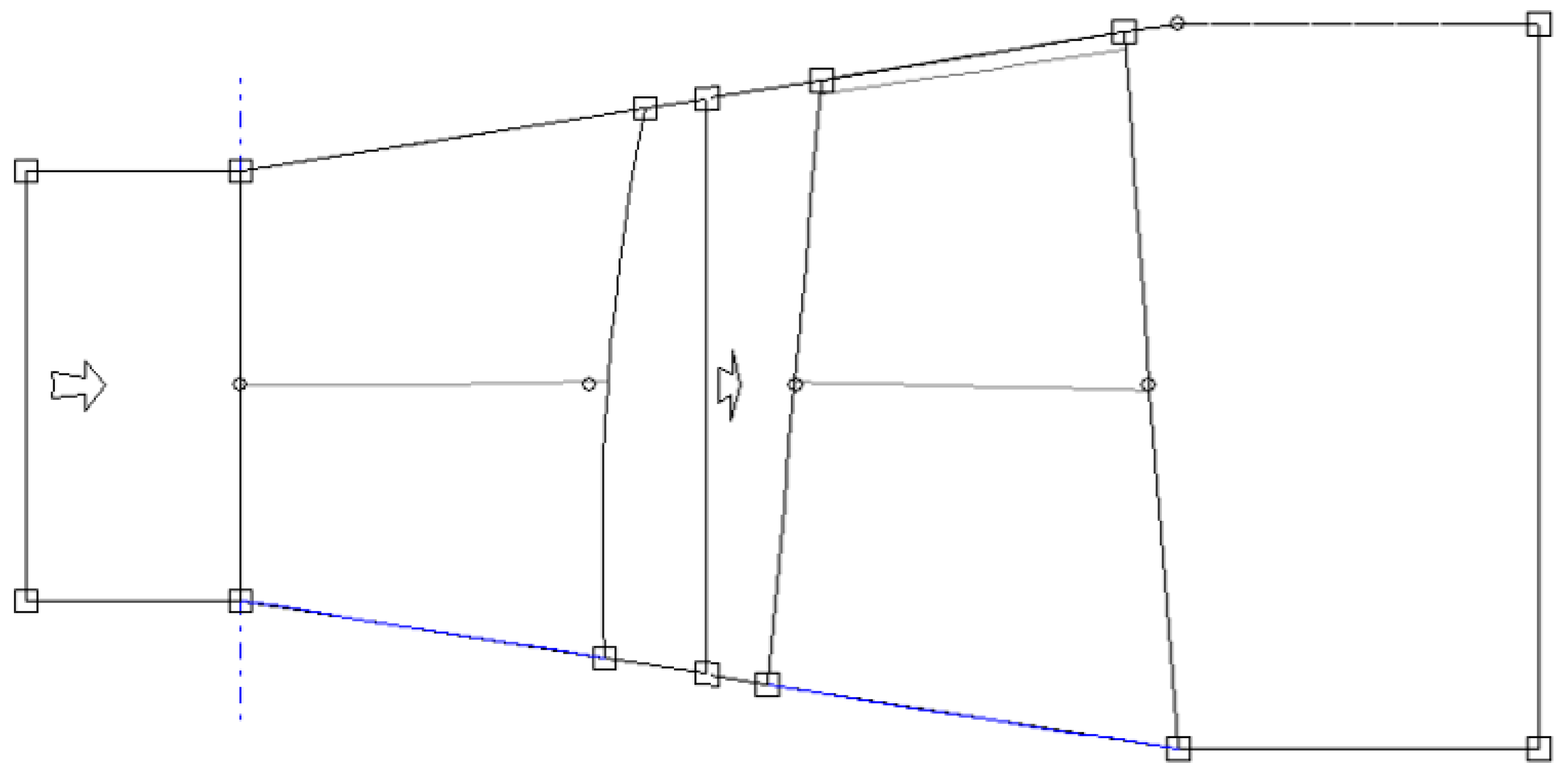
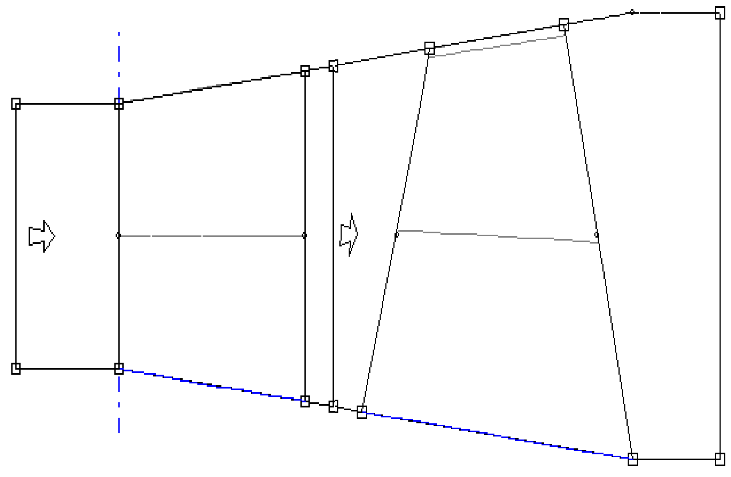
Figure 10 and Figure 11 below are a meridional side view of the blade profiles, visualising part of what is presented in Table 5. The more prominent difference when comparing the blade to the preliminary optimisation result, shown in Figure 11, is the stator tip being closer to the rotor. By guiding the flow further in the stage, the stator achieves faster speeds at rotor inlet, allowing more kinetic energy in the system, which can then be harvested by the rotor. Another important change in side view blade geometry is the dramatic change in chord length. Optimised blades tend to be shorter at hub and median layers and, as presented later, thicker. A possible explanation would be that flow through the blade would experience choking and considerable losses on longer blades, thus causing the chord reduction. Having thicker blades would increase the safety factor, as well as flow speed in the throat area, leading to possibly a more efficient energy harvesting mechanism.
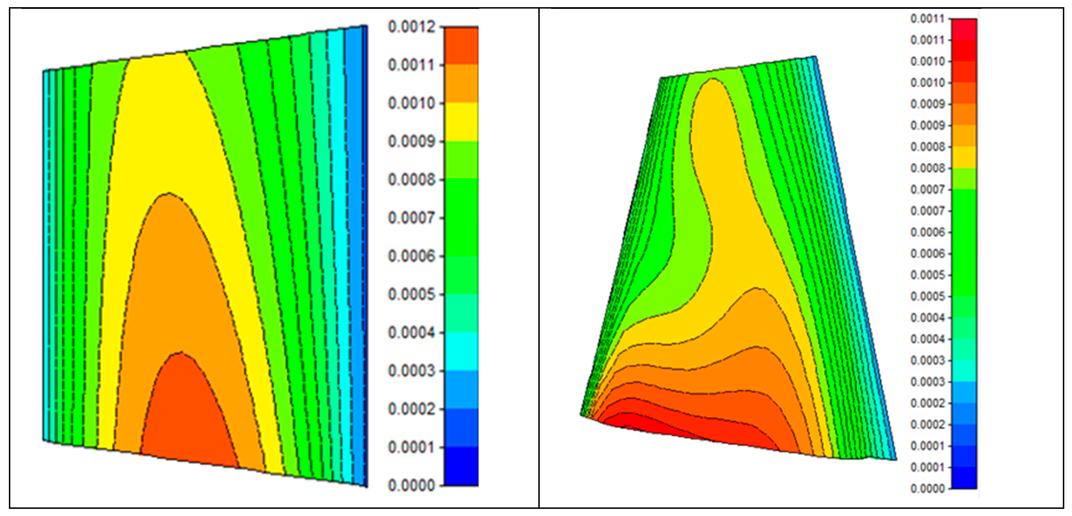
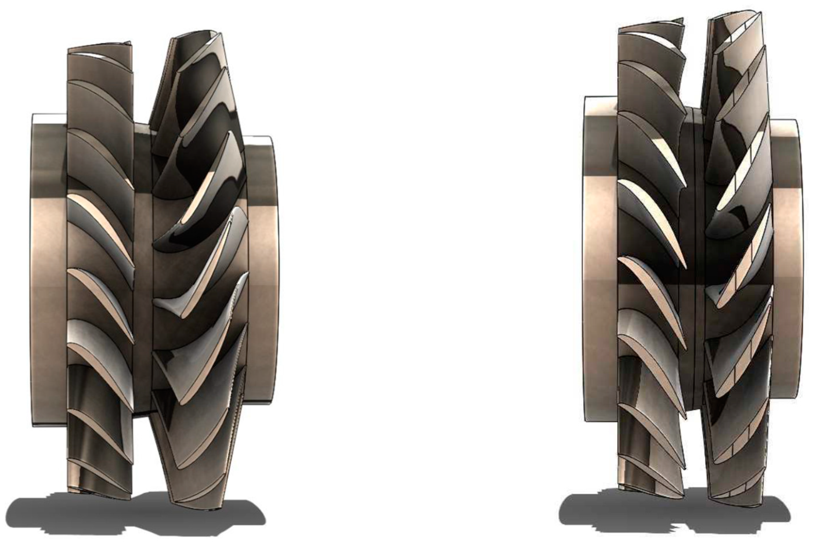
Figure 12 and Figure 13 show thickness contours for preliminary and optimised blades. The blade shape has consistently evolved towards higher thicknesses at stator centre, most likely to increase resistance to stresses applied by the flow. Constant chords were, as clearly shown and as expected, not optimised. The evolution trend shifted the trailing towards a shape that would better integrate with the rotor. The constant stator trailing edge thicknesses were heavily modified, however the ratios between layers were minimally modified. While this might be interpreted as a decisive result, stating that constant thicknesses were beneficial would not be advisable. The CFD simulations, along with the design evaluation algorithm were set up without a radial position based inlet speed, leading the flow to have similar characteristics throughout the stator. Realistic velocity distributions would likely lead to very different solutions, particularly regarding this parameter. In addition to this, the increase of upper rotor blade thickness is not common practice due to the potential to worsen the vibration of the rotor. However, this could be likely for one of two reasons. Firstly, a modal analysis was not included within the FEA due to the time additional time required, so theoretically a blade with poor vibrational characteristics could be deemed satisfactory by the fitness function. Alternatively, the methodology used does not consider common design practice when evaluating each population member. This prevents the restriction on potential design solutions, which conventionally would have been difficult to obtain. An overall view comparing preliminary to optimised geometry can be seen in Figure 14.

4.2. Parameter Evolutionary Behaviour

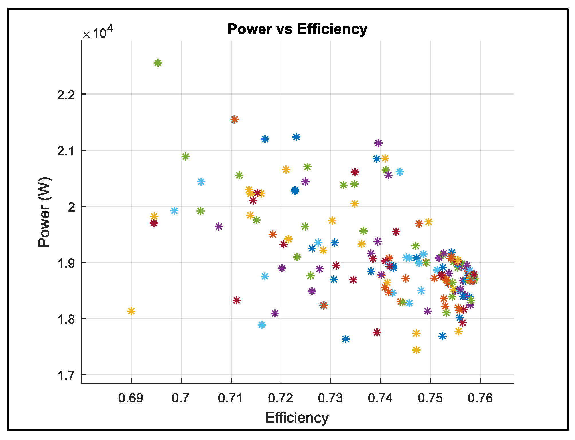
Figure 15 shows the power against efficiency plot for all blades that met the design constraints requirements. The graph shows a clear pattern of inverse proportionality, as well as the effect of the difference in weighting within the fitness function of these two parameters. The majority of designs were tending towards maximum efficiency, while still avoiding low power values. The graph highlights the effect of high penalisation fitness functions, with the genetic pool autonomously developing its own safety factor to prevent frequent fitness drops due to slight design changes. An ideal curve could be drawn to derive an empirical equation for power in function of efficiency, however, given the high dimensionality of the results, it would be an excessive approximation with limited practical use.
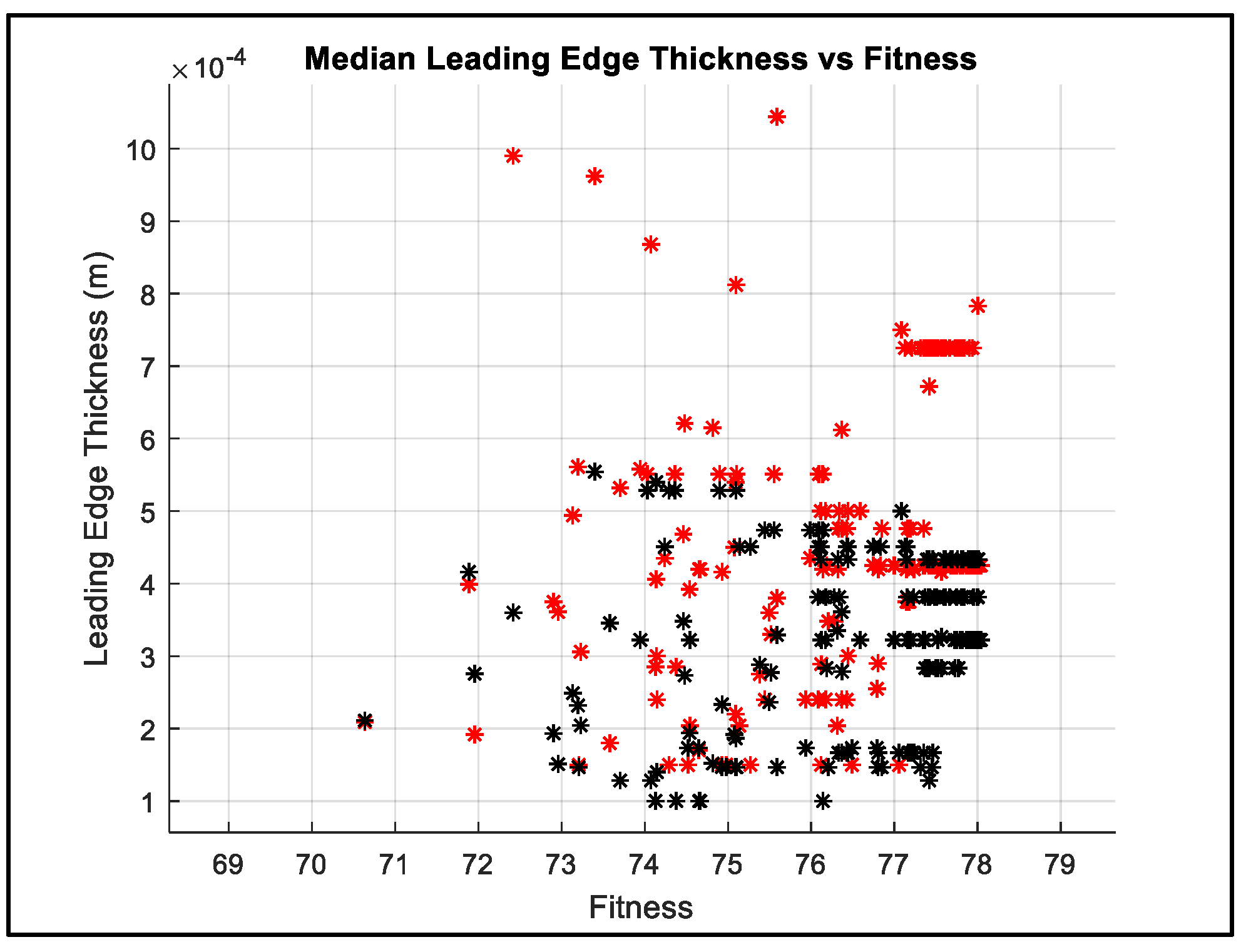
Median leading-edge thickness for rotor (red data points) and stator (black data points) scatter plots against fitness is shown in Figure 16. In terms of stator data analysis, it is clear that best fitness values correspond to thicknesses between 0.3 mm and 0.45 mm. Rotor data is divided in two different genetic types: best fitness values are found at 0.73 mm or at 0.42 mm. This could be interpreted as the genetic pool developing into two separate species, with different characteristics. High thickness elements feature slightly lower efficiencies, and greatly increased power. Lower thickness element, like the final result, feature significantly less power and marginally higher efficiency. This phenomenon occurred as a consequence of the multi-objective nature of the optimisation, and it is statistically likely that more parameters evolved into multiple species.
Figure 17 shows the elite member rotor leading edge thickness behaviour over the course of the optimisation. From this graph, one can observe the hub values convergence to higher values compared to the preliminary design analysis, to accommodate for the need of a higher rotor safety factor. Values for the median layer were initially increased, only to be minimised at a later stage of the optimisation. This behaviour is a consequence of the genetic pool prioritising low turbine failure rates, increasing influential parameters to ensure constraints compliance. In this case, the safety factor constraint was likely the cause for this increase. As blade parameters get optimised, failure rates sharply decreased, leading higher fitness elements with lower thicknesses to be more prominent. Tip values were influenced by median values behaviour; however, they clearly were not as influential in design constraints compliance.
Figure 18 shows the evolution pattern of stator axial chord. As generation number increases, hub and median values are minimised, while tip values stabilise at a value close to the initial guess. This shows a tendency towards shorter blade as the evidently provide better results. Hub and median values tend to the lower end of their respective ranges, thus suggesting that theoretical values for axial chords are not based on accurate empirical equations.
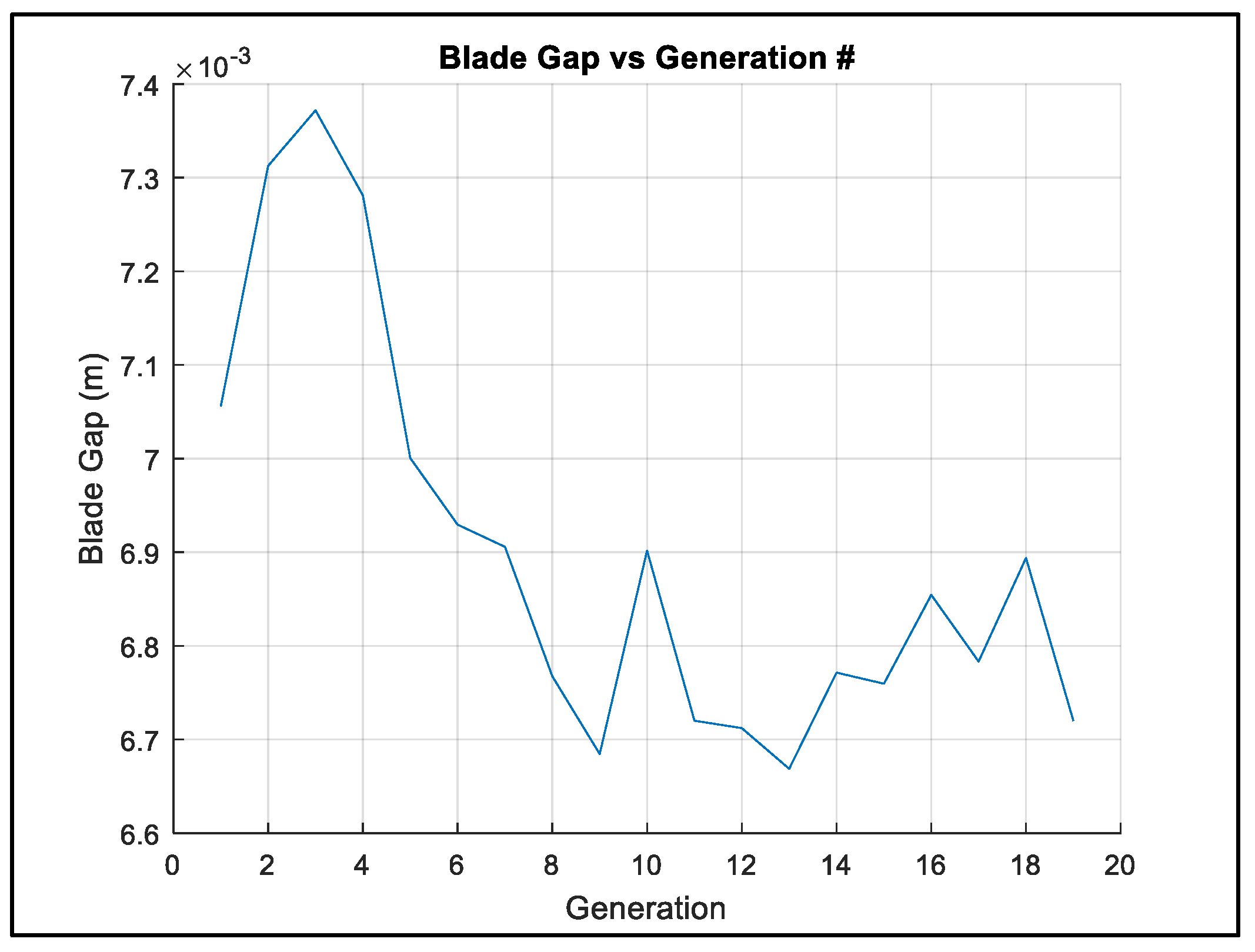
To provide a possible explanation to the phenomenon of unexpected stator axial chord, blade distance was plotted against generation number in Figure 18 and Figure 19, respectively. Blade distance was set up as a function of axial chords, and the graph shows this value being overestimated in preliminary design. It is probable that this parameter is so influential, that having worse than optimal values for all the dimensions that are included in the function used to estimate it is still beneficial.
Figure 20 is showing the rotor/stator stagger angle ratio at each layer. Values barely vary between generation 1 and generation 19, indicating either a complete non-influence of the parameter (simply impossible) on the turbine behaviour or that an optimum was already reached. It is important to note that it is highly likely that “optimum” simply means correlation with low blade failure rates. While further analysis should be carried out before coming to any conclusion, these findings are surely relevant. The magnitude of these values is also worth noting, with stagger angles ratios decreasing from hub to shroud. This could possibly be linked to different tangential speeds at each rotor layer, suggesting correlation between these two entities.

5. Conclusions

The use of numerical MDO and genetic algorithms is an extremely beneficial method for the aerodynamic shape optimisation of turbocharger turbines with many parameters. The dimensioning of this specific genetic algorithm (GA) has been applied to the specific problem and opportunity represented by axial turbine design for turbocharger application. Implementation of the GA has allowed for the improvement of the preliminary axial design in just over 4 h (2.73 day for a single computer) by only assessing 399 individual configurations. The final blade configuration achieved a total-to-static efficiency of 0.7587, an increment of 2.55% from the preliminary design, while providing a sufficient amount of power and implementing a higher safety factor.

Author Contributions

M.B., G.G. and G.W. were the research students who conducted the project at Brunel University London. A.P. is the turbomachinery group leader in the Centre of Advanced Powertrains and Fuels (CAPF) at Brunel University London, who conceived of the project, the layout of the investigations and checked the computational outcome of the resultant modelling effort and subsequent discussion.

Funding

This research has received funding from the Engineering and Physical Sciences Research Council Impact Acceleration Account.

Conflicts of Interest

The authors declare no conflict of interest.

Nomenclature

N b Bit size of every chromosome
N g e n Number of Generations
N i Population number
p m i s s Probability of a bit having the same value throughout the genetic pool
P m u t Mutation Rate
T s Chosen Tournament Size
Abbreviations
CFDComputational Fluid Dynamics
FEAFinite Element Analysis
GAGenetic Algorithm
MDOMultidisciplinary Design Optimisation

References

  1. Walsh, G.; Berchiolli, M.; Guarda, G.; Pesyridis, A. Turbocharger Axial Turbines for High Transient Response, Part 1: A Preliminary Design Methodology. Appl. Sci. 2019, 9, 838. [Google Scholar] [CrossRef]
  2. Poloni, C. Hybrid GA for multi objective aerodynamic shape optimization. In Genetic Algorithms in Engineering and Computer Science; John Wiley & Sons: New York, NY, USA, 1995; pp. 397–415. [Google Scholar]
  3. Nemec, M.; Zingg, D.W.; Pulliam, T.H. Multipoint and Multi-Objective Aerodynamic Shape Optimization. AIAA J. 2004, 42, 1057–1065. [Google Scholar] [CrossRef]
  4. Sobieszczanski-Sobiesk, J.; Haftka, R. Multidisciplinary aerospace design optimization: Survey of recent developments. Struct. Optim. 1997, 14, 1–23. [Google Scholar] [CrossRef]
  5. Pritchard, L. An Eleven Parameter Axial Turbine Airfoil Geometry Model. In Proceedings of the ASME 1985 International Gas Turbine Conference and Exhibit, Houston, TX, USA, 18–21 March 1985. [Google Scholar]
  6. Trigg, M.; Tubby, G.; Sheard, A. Automatic Genetic Optimization Approach to Two-Dimensional Blade Profile Design for Steam Turbines. J. Turbomach. 1999, 121, 11–17. [Google Scholar] [CrossRef]
  7. Öksüz, Ö.; Akmandor, İ.S. Multi-Objective Aerodynamic Optimization of Axial Turbine Blades Using a Novel Multilevel Genetic Algorithm. J. Turbomach. 2010, 132, 1–14. [Google Scholar] [CrossRef]
  8. Fonseca, C.M.; Fleming, P.J. An Overview of Evolutionary Algorithms in Multiobjective Optimization. Evol. Comput. 1995, 3, 1–16. [Google Scholar] [CrossRef]
  9. Google, Inc. “Google Scholar”. 2019. Available online: https://scholar.google.co.uk/scholar?as_vis=1&q=genetic+algorithm+optimization&hl=en&as_sdt=1,5&as_ylo=2018 (accessed on 3 March 2019).
  10. Sudholt, D. The Benefits of Population Diversity in Evolutionary Algorithms: A Survey of Rigorous Runtime Analyses; Cornell University: Ithaca, NY, USA, 2018. [Google Scholar]
  11. Qu, B.; Zhu, Y.; Jiao, Y.; Wu, M.; Suganthan, P.; Liang, J. A survey on multi-objective evolutionary algorithms for the solution of the environmental/economic dispatch problems. Swarm Evol. Comput. 2017, 38, 1–11. [Google Scholar] [CrossRef]
  12. Chan, C.; Bai, H.; He, D. Blade shape optimization of the Savonius wind turbine using a genetic algorithm. Appl. Energy 2018, 213, 148–157. [Google Scholar] [CrossRef]
  13. Zhang, X.; Song, X.; Qiu, W.; Yuan, Z.; You, Y.; Deng, N. Multi-objective optimization of Tension Leg Platform using evolutionary algorithm based on surrogate model. Ocean Eng. 2018, 148, 612–631. [Google Scholar] [CrossRef] [Green Version]
  14. Harris Corporation Computer Systems Divisions. High Performance Super-Minicomputers; Harris Corporation: Fort Lauderdale, FL, USA, 1981. [Google Scholar]
  15. Goel, S.; Cofer IV, J.I.; Singh, H. Turbine Airfoil Design Optimization. In Proceedings of the ASME 1996 International Gas Turbine and Aeroengine Congress and Exhibition, Birmingham, UK, 10–13 June 1996. [Google Scholar]
  16. Cravero, C.; Dawes, W.N. Throughflow Design Using an Automatic Optimisation Strategy. In Proceedings of the ASME 1997 International Gas Turbine and Aeroengine Congress and Exhibition, Orlando, FL, USA, 2–5 June 1997. [Google Scholar]
  17. Urdhwareshe, A. Object-Oriented Programming and its Concepts. Int. J. Innov. Sci. Res. 2016, 26, 1–6. [Google Scholar]
  18. Gutowski, M.W. Biology, Physics, Small Worlds and Genetic Algorithms. In Leading Edge Computer Science Research; Shannon, S., Ed.; Nova Science Publishers: Hauppauge, NY, USA, 2005; pp. 165–218. [Google Scholar]
  19. Alajmi, A.; Wright, J. Selecting the most efficient genetic algorithm sets in solving unconstrained building optimization problem. Int. J. Sustain. Built Environ. 2014, 3, 18–26. [Google Scholar] [CrossRef] [Green Version]
  20. Coley, D. Improving the Algorithm. In An Introduction to Genetic Algorithms for Scientists and World Scientific; World Scientific: Singapore, 1999. [Google Scholar]
  21. Chawdhry, P.K.; Roy, R.; Pant, R.K. Soft Computing in Engineering Design and Manufacturing, 1st ed.; Springer: Berlin/Heidelberg, Germany, 1998. [Google Scholar]
  22. Miller, B.L.; Goldberg, D.E. Genetic Algorithms, Tournament Selection, and the Effects of Noise. Complex Syst. 1995, 9, 193–212. [Google Scholar]
  23. The International Nickel Company. Alloy IN-738 Technical Data; The International Nickel Company: New York, NY, USA, 2002. [Google Scholar]
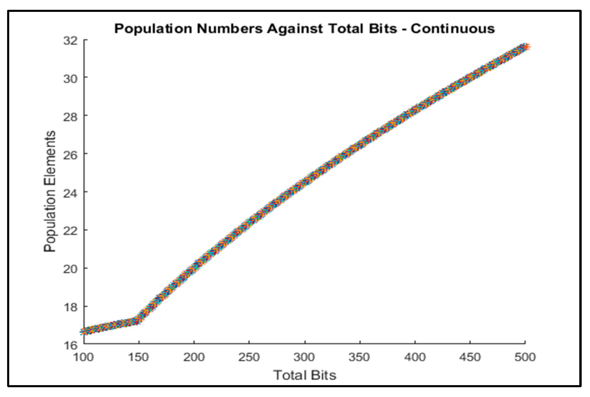
Figure 1. Growth of population size requirement with increasing chromosome bit size.
Applsci 09 02679 g001
Figure 2. Integer population size against total bits for total bits selection.
Applsci 09 02679 g002
Figure 3. Genetic variability overview for power generated.
Applsci 09 02679 g003
Figure 4. Schematic of crossover method implemented in the algorithm.
Applsci 09 02679 g004
Figure 5. Schematic of parent selection methodology, utilizing tournament selection, and elitism.
Applsci 09 02679 g005
Figure 6. Schematic outlining the design evaluation process used in ANSYS Workbench 18.1.
Applsci 09 02679 g006
Figure 7. Overview of CFD setup using ANSYS CFX turbo mode.
Applsci 09 02679 g007
Figure 8. Overview of finite element analysis (FEA) boundary conditions applied of stator (left) and rotor (right).
Applsci 09 02679 g008
Figure 9. Design space exploration by (a) efficiency, (b) average safety factor, (c) Mach number, (d) power, (e) elite fitness vs. generation number, and (f) elite fitness vs. generation number.
Applsci 09 02679 g009
Figure 10. Meridional side view of optimised blades.
Applsci 09 02679 g010
Figure 11. Meridional side view of preliminary blades.
Applsci 09 02679 g011
Figure 12. Meridional preliminary blade thickness contours (m) for (left) stator (right) rotor.
Applsci 09 02679 g012
Figure 13. Meridional optimised blade thickness contours (m) for (left) stator (right) rotor.
Applsci 09 02679 g013
Figure 14. Visual comparison between preliminary blade (left) and optimised blade (right) designs.
Applsci 09 02679 g014
Figure 15. Power against efficiency for all assessed configurations within design objective constraints.
Applsci 09 02679 g015
Figure 16. Leading edge thickness at the median layer vs. fitness for rotor (red) and stator (black).
Applsci 09 02679 g016
Figure 17. Elite member rotor leading edge thickness against generation number.
Applsci 09 02679 g017
Figure 18. Elite member stator axial chord against generation number.
Applsci 09 02679 g018
Figure 19. Elite member blade distance against the generation number.
Applsci 09 02679 g019
Figure 20. Elite member stagger angles ratio against generation number.
Applsci 09 02679 g020
Table 1. Final design constraints.
ParameterConstraint
Power (W)>17,000
Rotor Safety Factor>2
Stator Safety Factor>2
Global Maximum Mach Number<1.35
Table 2. Computational fluid dynamics (CFD) boundary conditions at design point [1].
Boundary ConditionsValue
Inlet Mass Flow Rate0.127238 kg/s
Inlet Total Temperature1168.55 K
Inlet Turbulence Intensity5%
Outlet Static Pressure1.30352 bar
Rotational Speed158,850 rpm
Table 3. Design evaluation timings.
Design Evaluation PhaseTime (s)
MATLAB script and Ansys Start-up92
File Reading and Importing75
CFD Analysis328
FSI Analysis (including CFD results importing)207
Total702
Table 4. Design optimisation final results.
Preliminary DesignOptimised DesignPercentage Change
Efficiency (T-s)73.98%75.87%+2.55%
Power (kW)20.318.79−7.44%
Rotor Safety Factor1.782.38+33.71%
Stator Safety Factor1.872.78+48.66%
Table 5. Comparison between preliminary parameters and optimised parameters.
Preliminary Design
StatorRotor
HubMeanTipHubMeanTip
Axial Chord (mm)6.436.436.439.366.934.63
Stagger Angle (°)48.9648.9648.9641.6456.4564.24
Chord (mm)9.799.799.7912.5212.5410.65
LE Wedge (°)262626242424
TE Wedge (°)444232
LE Thickness (mm)0.350.350.350.620.450.38
TE Thickness (mm)0.170.170.170.220.220.22
Optimised Design
StatorRotor
HubMeanTipHubMeanTip
Axial Chord (mm)6.065.816.726.815.875.03
Stagger Angle (°)45.3946.3552.377139.9852.2463.05
Chord (mm)8.638.4211.018.899.5911.10
LE Wedge (°)282728272727
TE Wedge (°)3.435.375.854.885.375.37
LE Thickness (mm)0.390.320.230.750.430.43
TE Thickness (mm)0.220.200.220.230.190.16
Percentage Change
StatorRotor
HubMeanTipHubMeanTip
Axial Chord (mm)−5.75%−9.64%4.51%−27.24%−15.30%8.64%
Stagger Angle (°)−7.29%−5.33%6.98%−3.99%−7.46%−1.85%
Chord (mm)−11.85%−13.99%12.46%−28.99%−23.52%4.23%
LE Wedge (°)7.69%3.85%7.69%12.50%12.50%12.50%
TE Wedge (°)−14.25%34.25%46.25%144.00%79.00%168.50%
LE Thickness (mm)11.43%−8.57%−34.29%20.97%−4.44%13.16%
TE Thickness (mm)29.41%17.65%29.41%4.55%−13.64%−27.27%