DC2Anet: Generating Lumbar Spine MR Images from CT Scan Data Based on Semi-Supervised Learning

 ,
,  ,
,  , ,
, ,
Abstract
1. Introduction
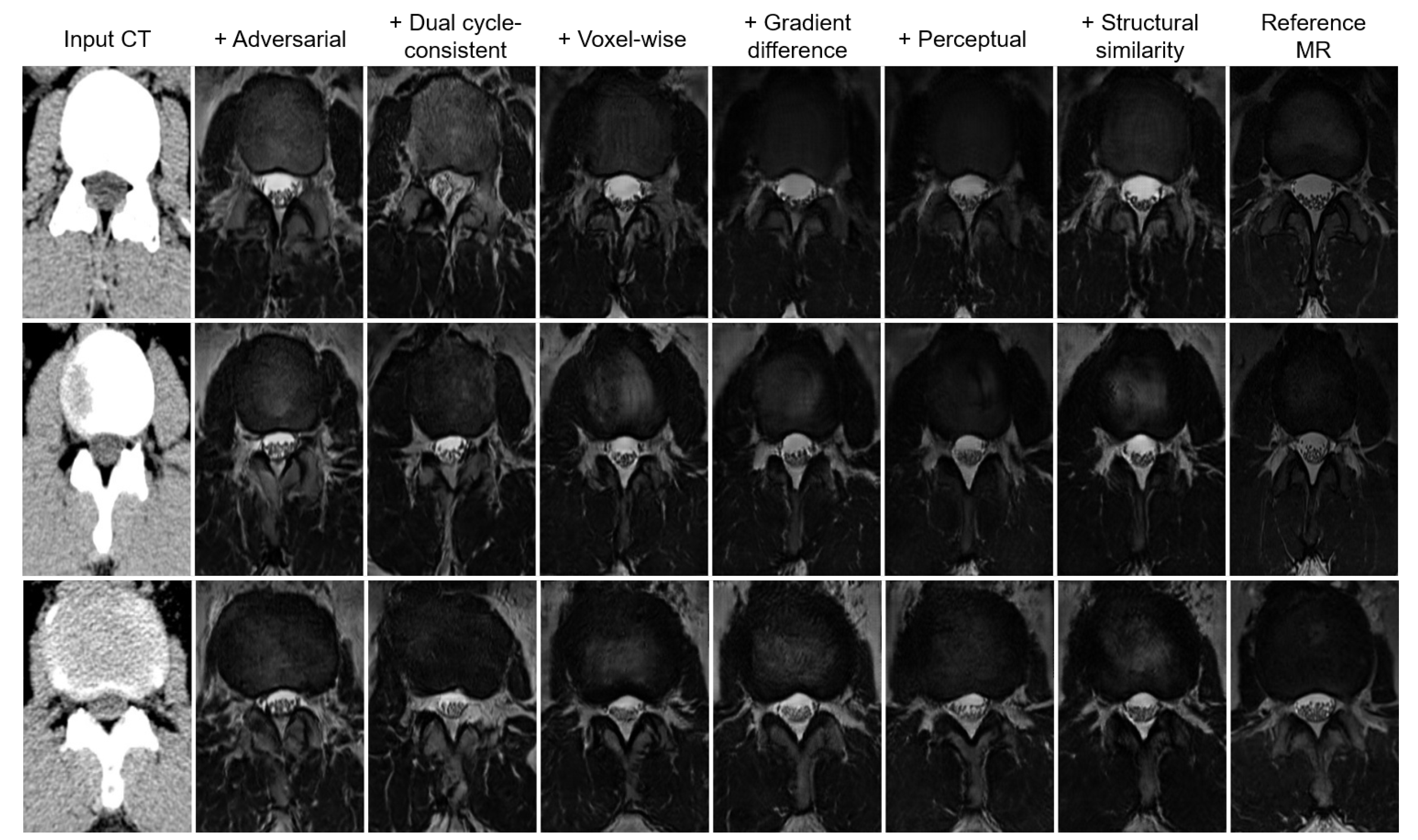
- An objective function is proposed to balance quantitative and qualitative loss terms to construct a realistic and accurate synthetic MR image. This function consists of adversarial, dual cycle-consistent, voxel-wise, gradient difference, perceptual, and structural similarity losses. Using ablation analysis, the importance and effectiveness of each of these loss terms are investigated.
- The dual cycle-consistent adversarial network (DCAnet) is proposed as a general synthesis system for semi-supervised learning. Due to its dual cycle-consistent structure, DCAnet can be applied to both supervised and unsupervised learning.
2. Literature Review of Medical Imaging Synthesis
3. Method
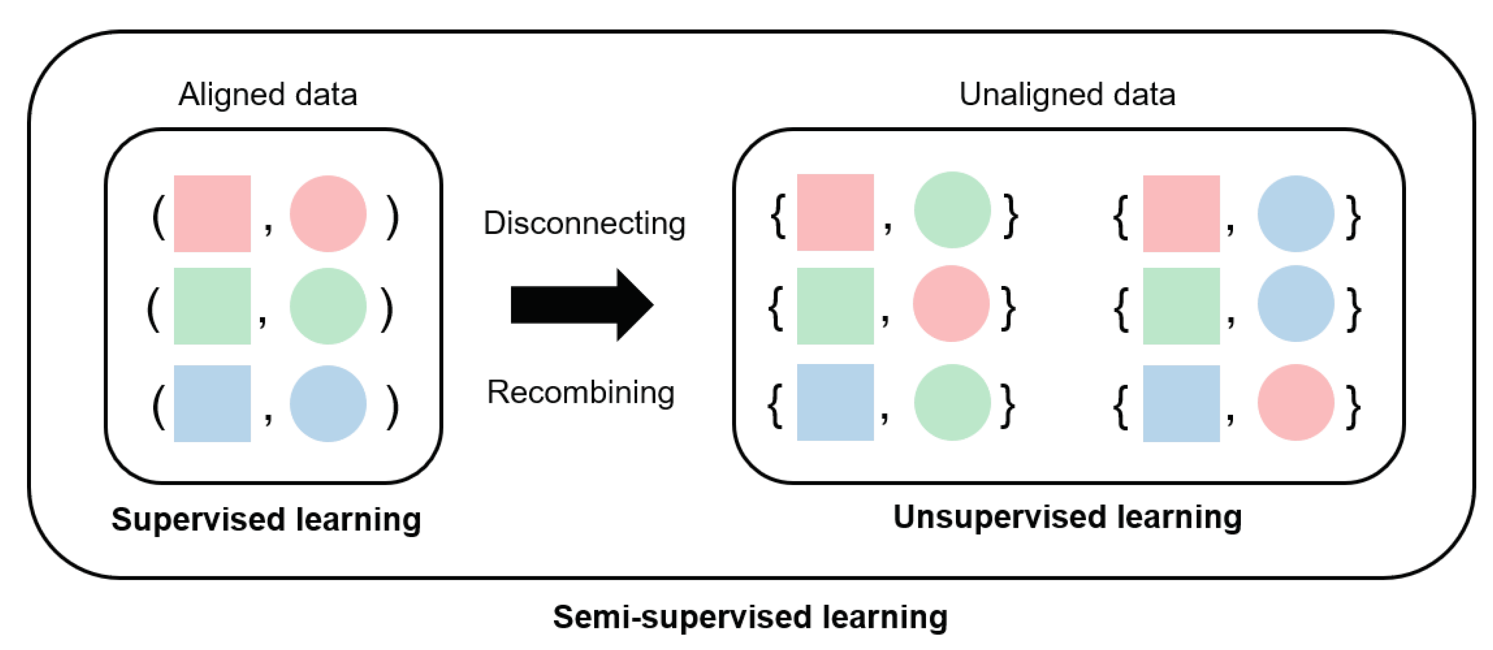
3.1. Converting Supervised Learning to Semi-Supervised Learning
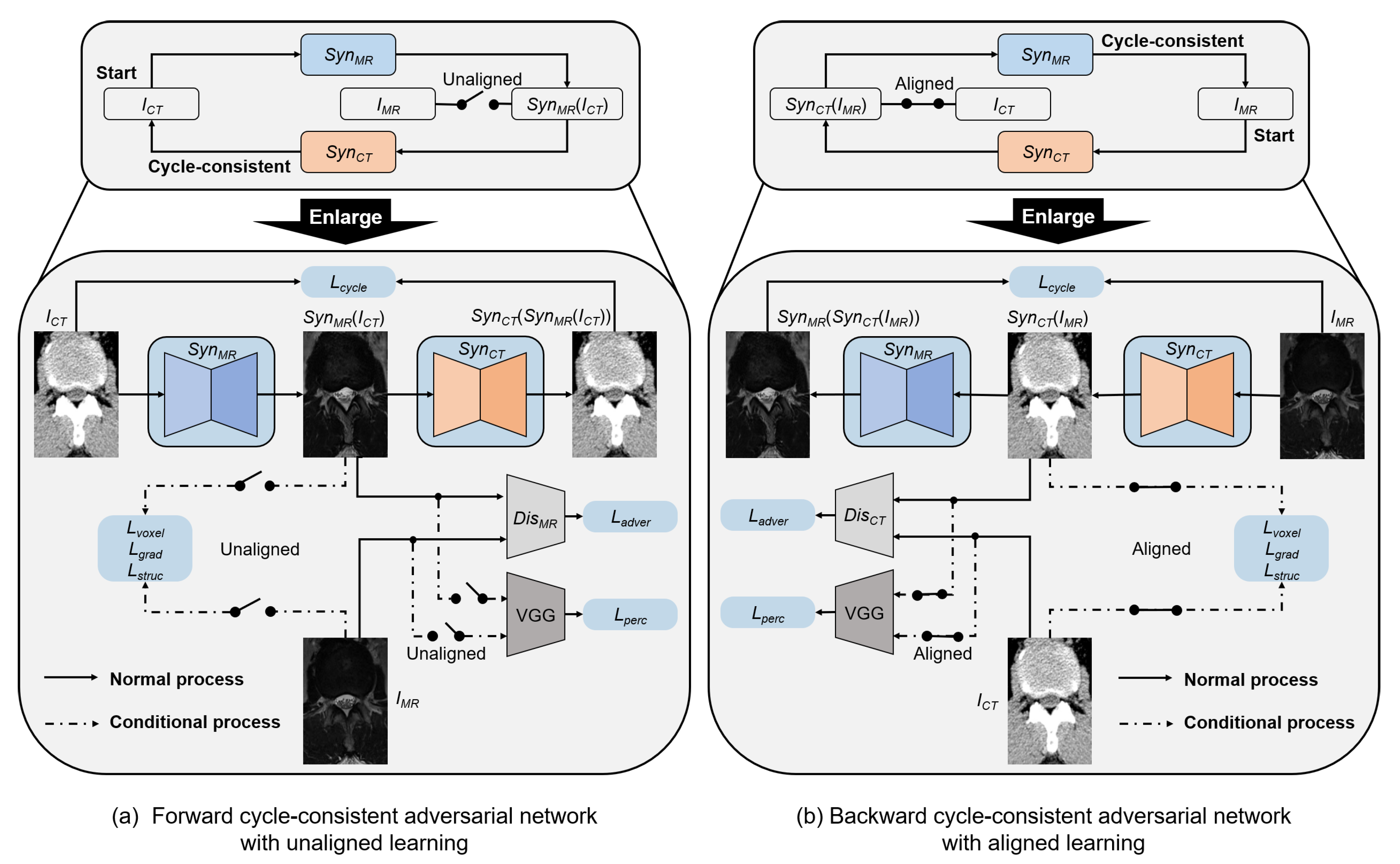
3.2. Dual Cycle-Consistent Adversarial Network
3.3. Objective Function
3.4. Optimization of DCAnet with Semi-Supervised Learning
- Joint optimization: For each training iteration, both the synthesis and discriminator networks are updated with regards to the objective function using supervised and unsupervised learning as defined in Equation (12). A pair of aligned data points and a pair of unaligned data points are sampled from the dataset and fed to DCAnet to update the networks.
- Alternating optimization: For each training iteration, supervised and unsupervised learning for the objective function are alternated as defined in Equations (10) and (11). In this case, only the weights that correspond to the synthesis networks and the particular layers of the discriminators are updated. This form of training maintains a more stable convergence of the optimization, and it is easy to balance the synthesis and discriminator networks with Jensen–Shannon divergence [3]. However, the computational load required for alternating optimization is nearly twice as high as that of joint optimization in the training stage.
| Algorithm 1 Mini-batch stochastic gradient descent training of DCAnet. We used default values of , , , , and . |
Require: The batch size m, the number of alternative iterations between supervised learning and unsupervised learning and , the learning rate , and Adam hyperparameters and .
|
3.5. Network Architecture
4. Experimental Results and Discussion
4.1. Implementation Details
4.2. Data Acquisition
4.3. Evaluation Metrics
4.4. Analysis of DCAnet
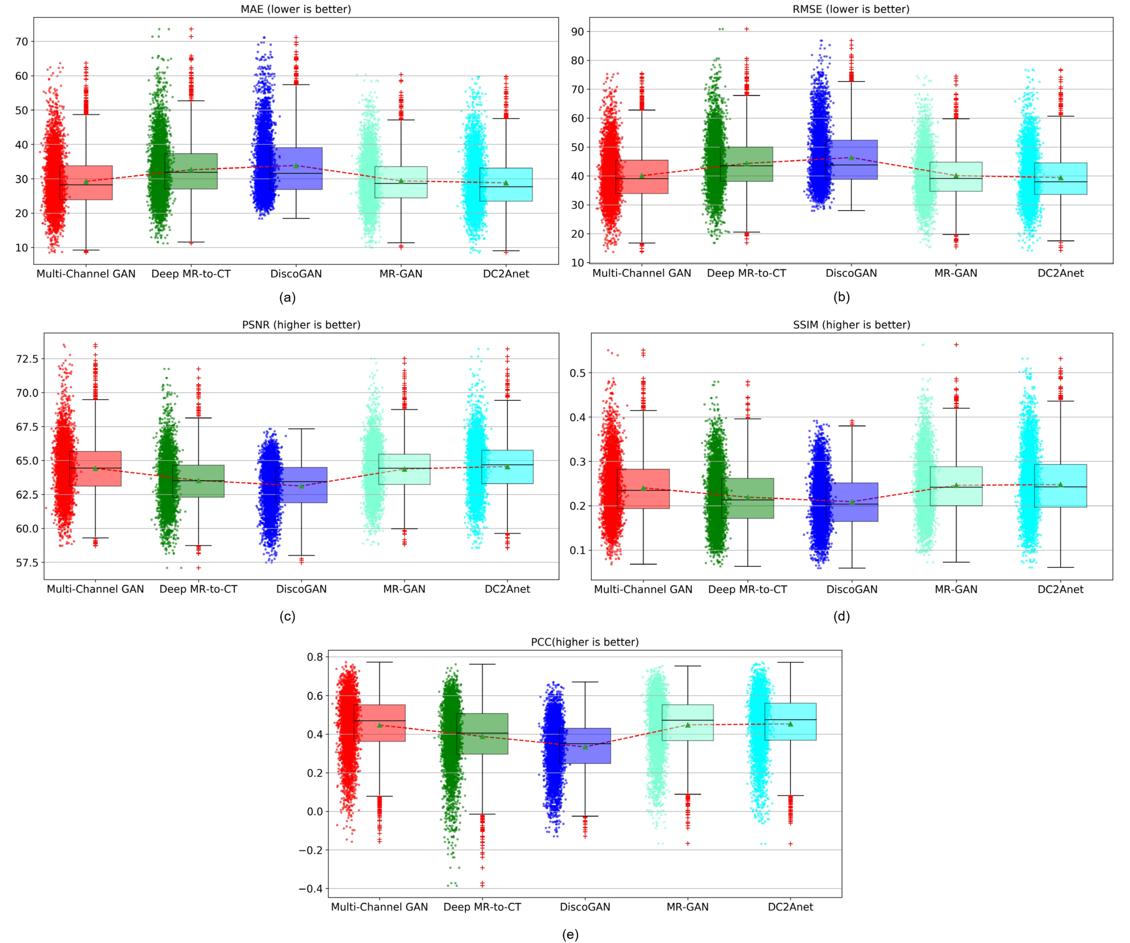
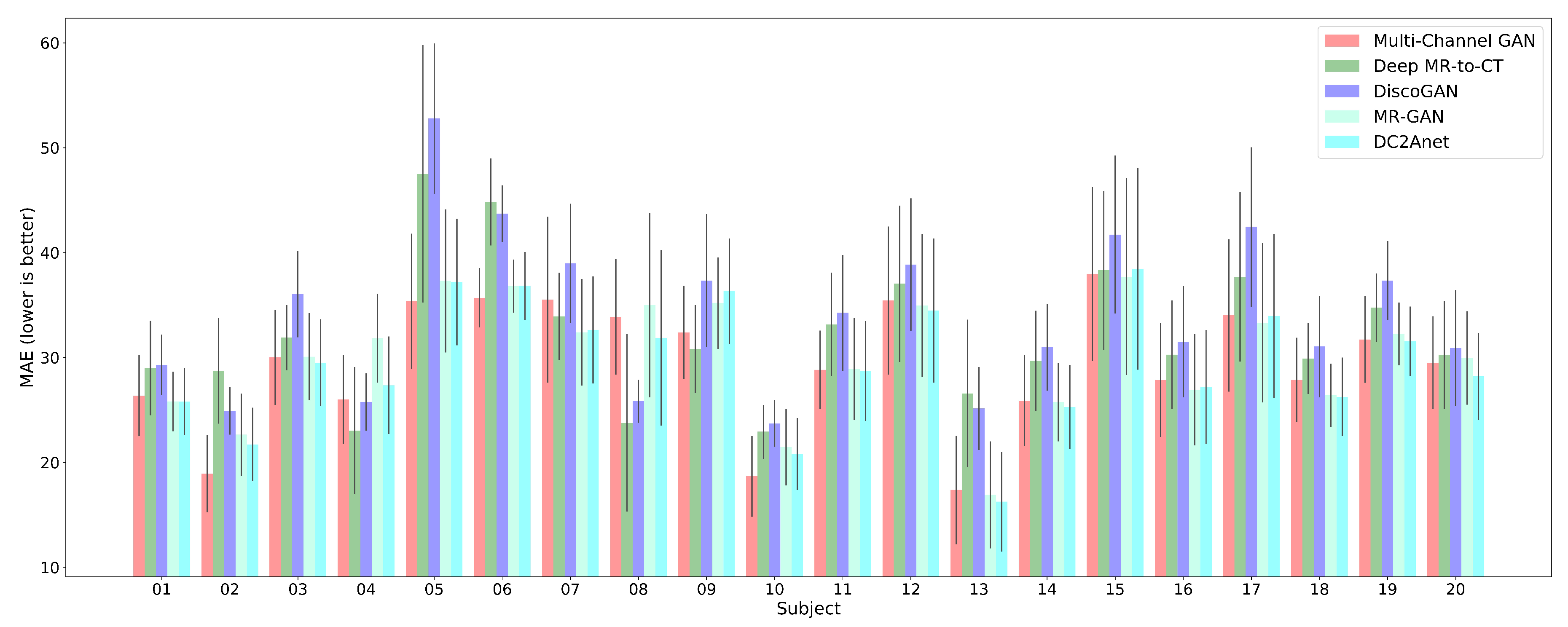
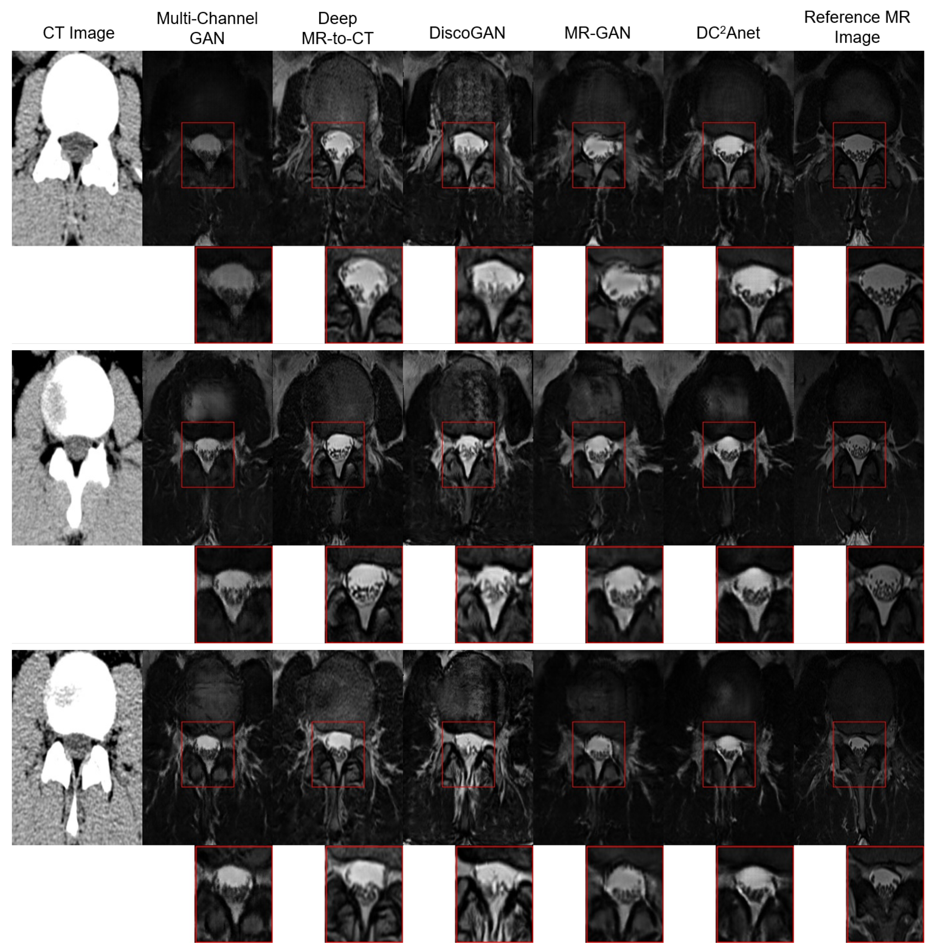
4.5. Comparison with Baselines
5. Conclusions
Author Contributions
Conflicts of Interest
References
- Krizhevsky, A.; Sutskever, I.; Hinton, G.E. Imagenet classification with deep convolutional neural networks. In Proceedings of the Advances in Neural Information Processing Systems, Lake Tahoe, USA, 3–8 December 2012; pp. 1097–1105. [Google Scholar]
- LeCun, Y.; Boser, B.; Denker, J.S.; Henderson, D.; Howard, R.E.; Hubbard, W.; Jackel, L.D. Backpropagation applied to handwritten zip code recognition. Neural Comput. 1989, 1, 541–551. [Google Scholar] [CrossRef]
- Goodfellow, I.; Pouget-Abadie, J.; Mirza, M.; Xu, B.; Warde-Farley, D.; Ozair, S.; Courville, A.; Bengio, Y. Generative adversarial nets. In Proceedings of the Advances in Neural Information Processing Systems, Montreal, QC, Canada, 8–13 December 2014; pp. 2672–2680. [Google Scholar]
- Hsu, S.H.; Cao, Y.; Huang, K.; Feng, M.; Balter, J.M. Investigation of a method for generating synthetic CT models from MRI scans of the head and neck for radiation therapy. Phys. Med. Biol. 2013, 58, 8419. [Google Scholar] [CrossRef] [PubMed]
- Zheng, W.; Kim, J.P.; Kadbi, M.; Movsas, B.; Chetty, I.J.; Glide-Hurst, C.K. Magnetic resonance–based automatic air segmentation for generation of synthetic computed tomography scans in the head region. Int. J. Radiat. Oncol. Biol. Phys. 2015, 93, 497–506. [Google Scholar] [CrossRef] [PubMed]
- Kapanen, M.; Tenhunen, M. T1/T2*-weighted MRI provides clinically relevant pseudo-CT density data for the pelvic bones in MRI-only based radiotherapy treatment planning. Acta Oncol. 2013, 52, 612–618. [Google Scholar] [CrossRef] [PubMed]
- Arjovsky, M.; Chintala, S.; Bottou, L. Wasserstein GAN. arXiv 2017, arXiv:1701.07875. [Google Scholar]
- Gulrajani, I.; Ahmed, F.; Arjovsky, M.; Dumoulin, V.; Courville, A.C. Improved training of Wasserstein GANs. In Proceedings of the Advances in Neural Information Processing Systems, Long Beach, CA, USA, 4–9 December 2017; pp. 5767–5777. [Google Scholar]
- Su, K.H.; Hu, L.; Stehning, C.; Helle, M.; Qian, P.; Thompson, C.L.; Pereira, G.C.; Jordan, D.W.; Herrmann, K.A.; Traughber, M.; et al. Generation of brain pseudo-CTs using an undersampled, single-acquisition UTE-mDixon pulse sequence and unsupervised clustering. Med. Phys. 2015, 42, 4974–4986. [Google Scholar] [CrossRef] [PubMed]
- Huynh, T.; Gao, Y.; Kang, J.; Wang, L.; Zhang, P.; Lian, J.; Shen, D. Estimating CT image from MRI data using structured random forest and auto-context model. IEEE Trans. Med. Imaging 2016, 35, 174–183. [Google Scholar] [CrossRef]
- Jog, A.; Carass, A.; Prince, J.L. Improving magnetic resonance resolution with supervised learning. In Proceedings of the 2014 IEEE 11th International Symposium on Biomedical Imaging (ISBI), Beijing, China, 29 April–2 May 2014; pp. 987–990. [Google Scholar]
- Catana, C.; van der Kouwe, A.; Benner, T.; Michel, C.J.; Hamm, M.; Fenchel, M.; Fischl, B.; Rosen, B.; Schmand, M.; Sorensen, A.G. Toward implementing an MRI-based PET attenuation-correction method for neurologic studies on the MR-PET brain prototype. J. Nucl. Med. 2010, 51, 1431–1438. [Google Scholar] [CrossRef]
- Andreasen, D.; Van Leemput, K.; Edmund, J.M. A patch-based pseudo-CT approach for MRI-only radiotherapy in the pelvis. Med. Phys. 2016, 43, 4742–4752. [Google Scholar] [CrossRef]
- Arabi, H.; Koutsouvelis, N.; Rouzaud, M.; Miralbell, R.; Zaidi, H. Atlas-guided generation of pseudo-CT images for MRI-only and hybrid PET–MRI-guided radiotherapy treatment planning. Phys. Med. Biol. 2016, 61, 6531. [Google Scholar] [CrossRef]
- Szegedy, C.; Liu, W.; Jia, Y.; Sermanet, P.; Reed, S.; Anguelov, D.; Erhan, D.; Vanhoucke, V.; Rabinovich, A. Going deeper with convolutions. In Proceedings of the IEEE Conference on Computer Vision and Pattern Recognition, Boston, MA, USA, 7–12 June 2015; pp. 1–9. [Google Scholar]
- Szegedy, C.; Vanhoucke, V.; Ioffe, S.; Shlens, J.; Wojna, Z. Rethinking the inception architecture for computer vision. In Proceedings of the IEEE Conference on Computer Vision and Pattern Recognition, Las Vegas, NV, USA, 27–30 June 2016; pp. 2818–2826. [Google Scholar]
- Tahmassebi, A.; Gandomi, A.H.; McCann, I.; Schulte, M.H.; Goudriaan, A.E.; Meyer-Baese, A. Deep learning in medical imaging: fMRI big data analysis via convolutional neural networks. In Proceedings of the PEARC’18, Pittsburgh, PA, USA, 22–26 July 2018. [Google Scholar]
- Esteva, A.; Kuprel, B.; Novoa, R.A.; Ko, J.; Swetter, S.M.; Blau, H.M.; Thrun, S. Dermatologist-level classification of skin cancer with deep neural networks. Nature 2017, 542, 115. [Google Scholar] [CrossRef] [PubMed]
- Dai, W.; Doyle, J.; Liang, X.; Zhang, H.; Dong, N.; Li, Y.; Xing, E.P. Scan: Structure correcting adversarial network for chest x-rays organ segmentation. arXiv 2017, arXiv:1703.08770. [Google Scholar]
- Son, J.; Park, S.J.; Jung, K.H. Retinal vessel segmentation in fundoscopic images with generative adversarial networks. arXiv 2017, arXiv:1706.09318. [Google Scholar]
- Alex, V.; KP, M.S.; Chennamsetty, S.S.; Krishnamurthi, G. Generative adversarial networks for brain lesion detection. In Medical Imaging 2017: Image Processing; International Society for Optics and Photonics: Bellingham, WA, USA, 2017; Volume 10133, p. 101330G. [Google Scholar]
- Han, X. MR-based synthetic CT generation using a deep convolutional neural network method. Med. Phys. 2017, 44, 1408–1419. [Google Scholar] [CrossRef] [PubMed]
- Ronneberger, O.; Fischer, P.; Brox, T. U-net: Convolutional networks for biomedical image segmentation. In International Conference on Medical Image Computing and Computer-Assisted Intervention, Munich, Germany, 5–9 October 2015; Springer: Munich, Germany, 2015; pp. 234–241. [Google Scholar]
- Simonyan, K.; Zisserman, A. Very deep convolutional networks for large-scale image recognition. arXiv 2014, arXiv:1409.1556. [Google Scholar]
- Mirza, M.; Osindero, S. Conditional generative adversarial nets. arXiv 2014, arXiv:1411.1784. [Google Scholar]
- Kingma, D.P.; Welling, M. Auto-encoding variational bayes. arXiv 2013, arXiv:1312.6114. [Google Scholar]
- Oord, A.v.d.; Kalchbrenner, N.; Kavukcuoglu, K. Pixel recurrent neural networks. arXiv 2016, arXiv:1601.06759. [Google Scholar]
- Radford, A.; Metz, L.; Chintala, S. Unsupervised representation learning with deep convolutional generative adversarial networks. arXiv 2015, arXiv:1511.06434. [Google Scholar]
- Zhao, J.; Mathieu, M.; LeCun, Y. Energy-based generative adversarial network. arXiv 2016, arXiv:1609.03126. [Google Scholar]
- Yeh, R.A.; Chen, C.; Yian Lim, T.; Schwing, A.G.; Hasegawa-Johnson, M.; Do, M.N. Semantic image inpainting with deep generative models. In Proceedings of the IEEE Conference on Computer Vision and Pattern Recognition, Honolulu, HI, USA, 21–26 July 2017; pp. 5485–5493. [Google Scholar]
- Wang, T.C.; Liu, M.Y.; Zhu, J.Y.; Liu, G.; Tao, A.; Kautz, J.; Catanzaro, B. Video-to-video synthesis. arXiv 2018, arXiv:1808.06601. [Google Scholar]
- Chan, C.; Ginosar, S.; Zhou, T.; Efros, A.A. Everybody dance now. arXiv 2018, arXiv:1808.07371. [Google Scholar]
- Bi, L.; Kim, J.; Kumar, A.; Feng, D.; Fulham, M. Synthesis of positron emission tomography (PET) images via multi-channel generative adversarial networks (GANs). In Molecular Imaging, Reconstruction and Analysis of Moving Body Organs, and Stroke Imaging and Treatment; Springer: Berlin/Heidelberg, Germany, 2017; pp. 43–51. [Google Scholar]
- Ben-Cohen, A.; Klang, E.; Raskin, S.P.; Amitai, M.M.; Greenspan, H. Virtual PET images from CT data using deep convolutional networks: Initial results. In International Workshop on Simulation and Synthesis in Medical Imaging; Springer: Cham, Switzerland, 2017; pp. 49–57. [Google Scholar]
- Long, J.; Shelhamer, E.; Darrell, T. Fully convolutional networks for semantic segmentation. In Proceedings of the IEEE Conference on Computer Vision and Pattern Recognition, Boston, MA, USA, 7–12 June 2015; pp. 3431–3440. [Google Scholar]
- Isola, P.; Zhu, J.Y.; Zhou, T.; Efros, A.A. Image-to-image translation with conditional adversarial networks. In Proceedings of the IEEE Conference on Computer Vision and Pattern Recognition, Honolulu, HI, USA, 21–26 July 2017; pp. 1125–1134. [Google Scholar]
- Nie, D.; Trullo, R.; Lian, J.; Petitjean, C.; Ruan, S.; Wang, Q.; Shen, D. Medical image synthesis with context-aware generative adversarial networks. In International Conference on Medical Image Computing and Computer-Assisted Intervention; Springer: Cham, Switzerland, 2017; pp. 417–425. [Google Scholar]
- Ji, S.; Xu, W.; Yang, M.; Yu, K. 3D convolutional neural networks for human action recognition. IEEE Trans. Pattern Anal. Mach. Intell. 2013, 35, 221–231. [Google Scholar] [CrossRef] [PubMed]
- Tran, D.; Bourdev, L.; Fergus, R.; Torresani, L.; Paluri, M. Learning spatiotemporal features with 3D convolutional networks. In Proceedings of the IEEE International Conference on Computer Vision, Santiago, Chile, 7–13 December 2015; pp. 4489–4497. [Google Scholar]
- Tu, Z.; Bai, X. Auto-context and its application to high-level vision tasks and 3D brain image segmentation. IEEE Trans. Pattern Anal. Mach. Intell. 2010, 32, 1744–1757. [Google Scholar] [PubMed]
- Wolterink, J.M.; Dinkla, A.M.; Savenije, M.H.; Seevinck, P.R.; van den Berg, C.A.; Išgum, I. Deep MR to CT synthesis using unpaired data. In International Workshop on Simulation and Synthesis in Medical Imaging; Springer: Cham, Switzerland, 2017; pp. 14–23. [Google Scholar]
- Zhu, J.Y.; Park, T.; Isola, P.; Efros, A.A. Unpaired image-to-image translation using cycle-consistent adversarial networks. In Proceedings of the IEEE International Conference on Computer Vision, Venice, Italy, 22–29 October 2017; pp. 2223–2232. [Google Scholar]
- Mao, X.; Li, Q.; Xie, H.; Lau, R.Y.; Wang, Z.; Paul Smolley, S. Least squares generative adversarial networks. In Proceedings of the IEEE International Conference on Computer Vision, Venice, Italy, 22–29 October 2017; pp. 2794–2802. [Google Scholar]
- Kim, T.; Cha, M.; Kim, H.; Lee, J.K.; Kim, J. Learning to discover cross-domain relations with generative adversarial networks. In Proceedings of the 34th International Conference on Machine Learning-Volume 70, Sydney, Australia, 6–11 August 2017; pp. 1857–1865. [Google Scholar]
- Jin, C.B.; Kim, H.; Liu, M.; Jung, W.; Joo, S.; Park, E.; Ahn, Y.S.; Han, I.H.; Lee, J.I.; Cui, X. Deep CT to MR synthesis using paired and unpaired data. Sensors 2019, 19, 2361. [Google Scholar] [CrossRef] [PubMed]
- He, K.; Zhang, X.; Ren, S.; Sun, J. Deep residual learning for image recognition. In Proceedings of the IEEE Conference on Computer Vision and Pattern Recognition, Las Vegas, NV, USA, 27–30 June 2016; pp. 770–778. [Google Scholar]
- He, K.; Zhang, X.; Ren, S.; Sun, J. Identity mappings in deep residual networks. In European Conference on Computer Vision; Springer: Cham, Switzerland, 2016; pp. 630–645. [Google Scholar]
- Johnson, J.; Alahi, A.; Fei-Fei, L. Perceptual losses for real-time style transfer and super-resolution. In European Conference on Computer Vision; Springer: Cham, Switzerland, 2016; pp. 694–711. [Google Scholar]
- Gatys, L.A.; Ecker, A.S.; Bethge, M. Image style transfer using convolutional neural networks. In Proceedings of the IEEE Conference on Computer Vision and Pattern Recognition, Las Vegas, NV, USA, 27–30 June 2016; pp. 2414–2423. [Google Scholar]
- Mahendran, A.; Vedaldi, A. Understanding deep image representations by inverting them. In Proceedings of the IEEE Conference on Computer Vision and Pattern Recognition, Boston, MA, USA, 7–12 June 2015; pp. 5188–5196. [Google Scholar]
- Wang, Z.; Bovik, A.C.; Sheikh, H.R.; Simoncelli, E.P. Image quality assessment: From error visibility to structural similarity. IEEE Trans. Image Process. 2004, 13, 600–612. [Google Scholar] [CrossRef] [PubMed]
- Wang, Z.; Bovik, A.C. Mean squared error: Love it or leave it? A new look at signal fidelity measures. IEEE Signal Process. Mag. 2009, 26, 98–117. [Google Scholar] [CrossRef]
- Sundaram, N.; Brox, T.; Keutzer, K. Dense point trajectories by GPU-accelerated large displacement optical flow. In European Conference on Computer Vision; Springer: Cham, Switzerland, 2010; pp. 438–451. [Google Scholar]
- Zach, C.; Klopschitz, M.; Pollefeys, M. Disambiguating visual relations using loop constraints. In Proceedings of the 2010 IEEE Computer Society Conference on Computer Vision and Pattern Recognition, San Francisco, CA, USA, 13–18 June 2010; pp. 1426–1433. [Google Scholar]
- Russakovsky, O.; Deng, J.; Su, H.; Krause, J.; Satheesh, S.; Ma, S.; Huang, Z.; Karpathy, A.; Khosla, A.; Bernstein, M. Imagenet large scale visual recognition challenge. Int. J. Comput. Vis. 2015, 115, 211–252. [Google Scholar] [CrossRef]
- Ulyanov, D.; Vedaldi, A.; Lempitsky, V. Instance normalization: The missing ingredient for fast stylization. arXiv 2016, arXiv:1607.08022. [Google Scholar]
- Maas, A.L.; Hannun, A.Y.; Ng, A.Y. Rectifier nonlinearities improve neural network acoustic models. In Proc. icml; Stanford Artificial Intelligence Laboratory: Stanford, CA, USA, 2013; Volume 30, p. 3. [Google Scholar]
- Xu, B.; Wang, N.; Chen, T.; Li, M. Empirical evaluation of rectified activations in convolutional network. arXiv 2015, arXiv:1505.00853. [Google Scholar]
- Shrivastava, A.; Pfister, T.; Tuzel, O.; Susskind, J.; Wang, W.; Webb, R. Learning from simulated and unsupervised images through adversarial training. In Proceedings of the IEEE Conference on Computer Vision and Pattern Recognition, Honolulu, HI, USA, 21–26 July 2017; pp. 2107–2116. [Google Scholar]
- Keskar, N.S.; Socher, R. Improving generalization performance by switching from Adam to SGD. arXiv 2017, arXiv:1712.07628. [Google Scholar]
- Tahmassebi, A. ideeple: Deep learning in a flash. In Disruptive Technologies in Information Sciences; International Society for Optics and Photonics: Bellingham, WA, USA, 2018; Volume 10652, p. 106520S. [Google Scholar]
- Tahmassebi, A.; Gandomi, A.H.; Fong, S.; Meyer-Baese, A.; Foo, S.Y. Multi-stage optimization of a deep model: A case study on ground motion modeling. PLoS ONE 2018, 13, e0203829. [Google Scholar] [CrossRef] [PubMed]
- Kingma, D.P.; Ba, J. Adam: A method for stochastic optimization. arXiv 2014, arXiv:1412.6980. [Google Scholar]


| CT Scans | MRI | |
|---|---|---|
| Principle | Uses multiple X-rays, taken at different angles to produce cross-sectional images | Uses powerful magnetic fields and radiofrequency pulses to produce detailed images |
| Radiation | Minimal | None |
| Uses | Excellent for observing bone and very good for soft tissue, especially with the use of intravenous contrast dye | Excellent for detecting very slight differences in soft tissue |
| Cost | Usually less expensive than MRI | Often more expensive than CT scans |
| Time taken | Very quick, taking only about 5 min, depending on the area being scanned | Depends on the part of the body being examined and can range from 15 min–2 h |
| Application | Produces a general image of an area such as internal organs, fractures, or head trauma | Produces more detailed images of soft tissue, ligaments, and organs |
| Benefits | Faster and can provide images of tissue, organs, and skeletal structure | Produces more detailed images |
| Risks |
|
|
| DCNN [22] | Multi-channel GAN [33] | Context-Aware GAN [37] | Deep MR-to-CT [41] | DiscoGAN [44] | MR-GAN [45] | |
|---|---|---|---|---|---|---|
| Application | Brain MR to CT | Lung CT to PET | Brain and pelvic MRI to CT | Brain MR to CT | Attribute translation | Brain CT to MRI |
| Objective function | Voxel-wise | Adversarial [25] and voxel-wise | Adversarial [25], voxel-wise, and gradient difference [37] | Least- squares adversarial [43] and cycle- consistent [42] | Adversarial [25] and cycle- consistent [42] | Adversarial [25], voxel -wise, and dual cycle- consistent [45] |
| Model | Pretrained VGG16 [24] with U-Net [23] | pix2pix [36] | 3D ConvNet [38,39] and auto-context model [40] | cycleGAN [42] | DiscoGAN [44] | MR-GAN [45] |
| No. of trainable parameters | M | M | Unknown | M | M | M |
| Generator | U-Net [23] | U-Net [23] | Customized | Residual Net [46,47,48] | Customized | Residual Net [46,47,48] |
| No. of layers in the generator | 27 | 16 | 8 | 24 | 8 | 24 |
| Discriminator | None | Patch GAN [36] | Customized | Path GAN [36] | Path GAN [36] | Path GAN [36] |
| No. of layers in the discriminator | None | 5 | 6 | 5 | 5 | 5 |
| Generation time | ms. | ms. | Unknown | ms. | ms. | ms. |
| Loss term | Strengths | Weaknesses | Aligned Data |
|---|---|---|---|
| Adversarial | Realistic output | Unstable training | ✗ |
| Ducal cycle-consistent | Possible unsupervised learning | Heavy computational load (two synthesis and two discriminator networks) | ✗ |
| Voxel-wise | Encourage the output similar to the reference image | Tends to produce blurry output | ✓ |
| Gradient difference | Emphasizes the boundaries of the output | Sensitive to the quality of data alignment | ✓ |
| Perceptual | Preserves high-level semantic similarity | Not a fully-analyzed and task-oriented problem | ✓ |
| Structural similarity | Relaxes misalignment constraints for data alignment | Prefers low illumination | ✓ |
| Layer Name/Type | Output Size | Filter Size/Stride | Number of Conv. Layers | Number of Parameters |
|---|---|---|---|---|
| Input image | None | 0 | 0 | |
| Conv 1, IN | /1 | 1 | 3200 | |
| Conv 2, IN | /2 | 1 | ||
| Conv 3, IN | /2 | 1 | ||
| Residual Block 1, IN | /2 | 2 | ||
| Residual Block 2, IN | /2 | 2 | ||
| Residual Block 3, IN | /2 | 2 | ||
| Residual Block 4, IN | /2 | 2 | ||
| Residual Block 5, IN | /2 | 2 | ||
| Residual Block 6, IN | /2 | 2 | ||
| Residual Block 7, IN | /2 | 2 | ||
| Residual Block 8, IN | /2 | 2 | ||
| Residual Block 9, IN | /2 | 2 | ||
| Fractional Conv 1, IN | / | 1 | ||
| Fractional Conv 2, IN | / | 1 | ||
| Conv 4, Tanh | /1 | 1 | 3137 | |
| Total number of parameters | 6,054,913 | |||
| Total number of parameters if instance normalization is applied | 6,065,217 | |||
| Number of Patients | Number of Slices | |
|---|---|---|
| Training set | 549 | 22,428 |
| Test set | 92 | 4426 |
| Total | 641 | 26,854 |
| Learning | Optimization | MAE | RMSE | PSNR | SSIM | PCC |
|---|---|---|---|---|---|---|
| Supervised | − | |||||
| Unsupervised | − | |||||
| Semi-supervised | Joint | |||||
| Semi-supervised | Alternating |
| Discriminator | MAE | RMSE | PSNR | SSIM | PCC |
|---|---|---|---|---|---|
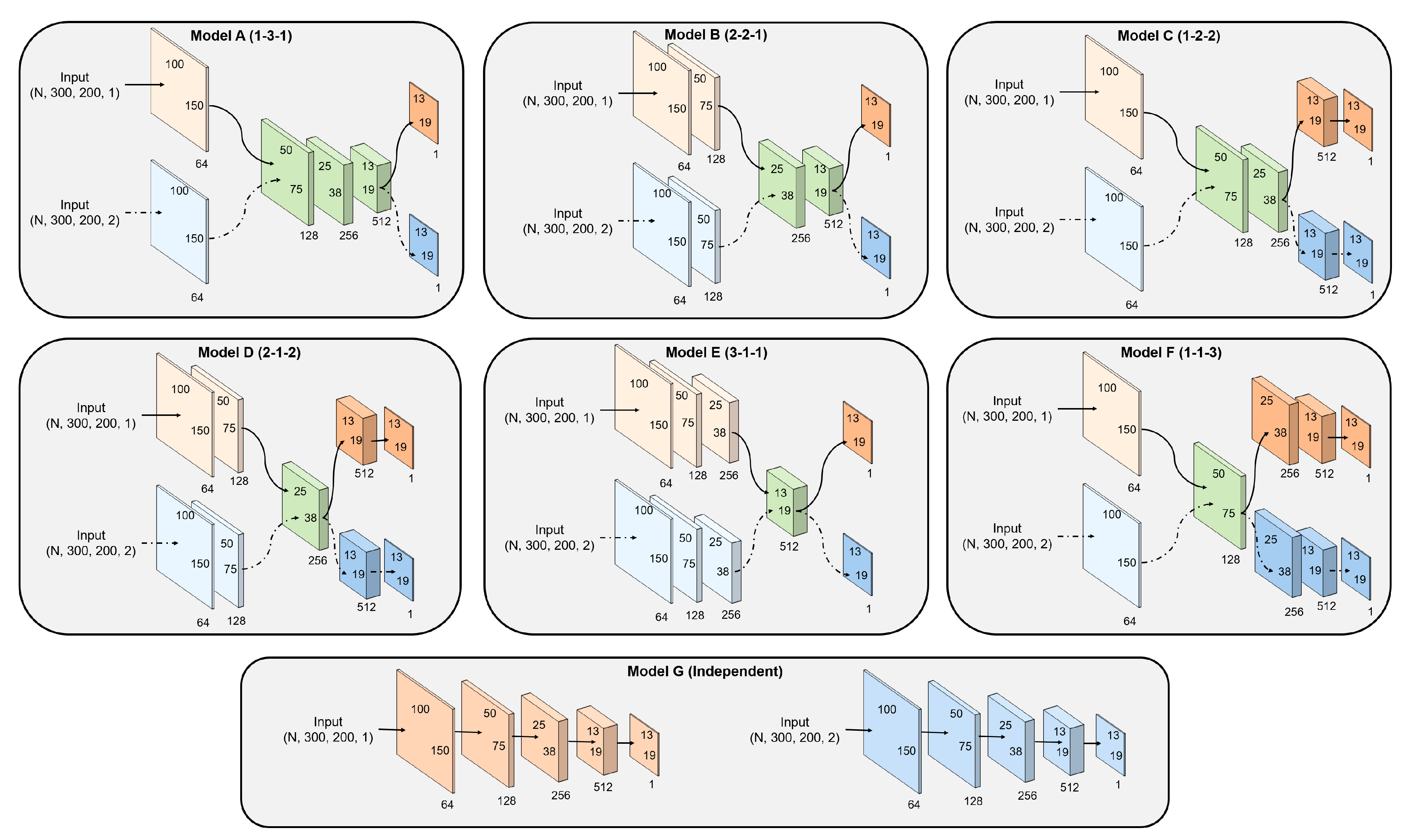
| Model A | |||||
| Model B | |||||
| Model C | |||||
| Model D | |||||
| Model E | |||||
| Model F | |||||
| Model G |
| Perceptual Layers | MAE | RMSE | PSNR | SSIM | PCC |
|---|---|---|---|---|---|
| ReLU | |||||
| ReLU | |||||
| ReLU | |||||
| ReLU | |||||
| ReLU |
| Objectives | MAE | RMSE | PSNR | SSIM | PCC | Relative MAE Improvement |
|---|---|---|---|---|---|---|
| Adversarial alone | ||||||
| + Dual cycle-consistent | ||||||
| + Voxel-wise | ||||||
| + Gradient difference | ||||||
| + Perceptual | ||||||
| + Structural similarity |
| Methods | MAE | RMSE | PSNR | SSIM | PCC |
|---|---|---|---|---|---|
| Multi-Channel GAN [33] | |||||
| Deep MR-to-CT [41] | |||||
| DiscoGAN [44] | |||||
| MR-GAN [45] | |||||
| DCAnet |
© 2019 by the authors. Licensee MDPI, Basel, Switzerland. This article is an open access article distributed under the terms and conditions of the Creative Commons Attribution (CC BY) license (http://creativecommons.org/licenses/by/4.0/).
Share and Cite
Jin, C.-B.; Kim, H.; Liu, M.; Han, I.H.; Lee, J.I.; Lee, J.H.; Joo, S.; Park, E.; Ahn, Y.S.; Cui, X. DC2Anet: Generating Lumbar Spine MR Images from CT Scan Data Based on Semi-Supervised Learning. Appl. Sci. 2019, 9, 2521. https://doi.org/10.3390/app9122521
Jin C-B, Kim H, Liu M, Han IH, Lee JI, Lee JH, Joo S, Park E, Ahn YS, Cui X. DC2Anet: Generating Lumbar Spine MR Images from CT Scan Data Based on Semi-Supervised Learning. Applied Sciences. 2019; 9(12):2521. https://doi.org/10.3390/app9122521
Chicago/Turabian StyleJin, Cheng-Bin, Hakil Kim, Mingjie Liu, In Ho Han, Jae Il Lee, Jung Hwan Lee, Seongsu Joo, Eunsik Park, Young Saem Ahn, and Xuenan Cui. 2019. "DC2Anet: Generating Lumbar Spine MR Images from CT Scan Data Based on Semi-Supervised Learning" Applied Sciences 9, no. 12: 2521. https://doi.org/10.3390/app9122521
APA StyleJin, C.-B., Kim, H., Liu, M., Han, I. H., Lee, J. I., Lee, J. H., Joo, S., Park, E., Ahn, Y. S., & Cui, X. (2019). DC2Anet: Generating Lumbar Spine MR Images from CT Scan Data Based on Semi-Supervised Learning. Applied Sciences, 9(12), 2521. https://doi.org/10.3390/app9122521