Article

System for Evaluation and Compensation of Leg Length Discrepancy for Human Body Balancing

1
Mechatronics Department, Bjelovar University of Applied Sciences, 43000 Bjelovar, Croatia
2
Cognitus Ltd., 10000 Zagreb, Croatia
3
Akromion—Special Hospital for Orthopaedic Surgery, 49217 Krapinske Toplice, Croatia
4
Laboratory for Robotics and Intelligent Control Systems (LARICS), Faculty of Electrical Engineering and Computing, University of Zagreb, 10000 Zagreb, Croatia
*
Author to whom correspondence should be addressed.
Appl. Sci. 2019, 9(12), 2504; https://doi.org/10.3390/app9122504
Submission received: 8 May 2019 / Revised: 9 June 2019 / Accepted: 17 June 2019 / Published: 19 June 2019
(This article belongs to the Section Mechanical Engineering)

Abstract

:
Leg Length Discrepancy (LLD) causes a shift of the Center of Mass (CoM) of the human body, as well as an asymmetry in load distribution on the lower extremities. Existing LLD evaluation methods do not take into account this shift in the human body’s CoM. In this paper, a methodology and mechatronic system for the Evaluation and Compensation of LLD for Human Body Balancing are described. The human body’s CoM is measured with two force plates located on two parallel manipulators. Since persons with LLD experience a shift in their CoM, by raising the force plate that is under the shorter leg, the human body can be balanced. For this purpose, the Human Body Balancing Algorithm (HBBA) was proposed and developed. By running the HBBA, the height difference between the force plates under the left and right leg can be measured, which then represents the LLD evaluation. Based on this evaluation, it is possible to design and make a shoe insole which compensates the influence of LLD with the goal of equalizing the load on the legs. A virtual mathematical model of the system was created and the simulation results of the HBBA are presented. The mechatronic system, developed and used to conduct experiments and measurements, is described in detail.

1. Introduction

Anisomelia or limb length discrepancy is an orthopedic condition involving significant inequality between paired limbs. Inequality between lower extremities is known as Leg Length Discrepancy (LLD). LLD affects the patients’ quality of life due to several functional activities such as posture, balance [1,2], walking [3,4,5] and running [6] being disrupted.
If the LLD amounts to over 20 mm, it is considered to be significant, and what is concerning is that this condition occurs in 0.1% of the world’s population [2]. With regards to etiology, LLD is classified as structural or functional. Structural or anatomical LLD is defined as a difference in leg length caused by unequal bone structure. Functional or apparent LLD is defined as a mechanical change in the lower extremities, such as varus and valgus deformities of knees and feet, as well as scoliosis of the spine [7]. Even though our system allows for detection of functional LLD, in this study, we focused on anatomical LLD and prepared the system for clinical trials on this particular problem. In our future research, we plan to investigate functional LLD by determining mathematical models and methods for changing roll and pitch of moving platforms, thus allowing practitioners to determine status of functional LLD. Moreover, the mechanical design of the proposed system is based on parallel manipulators that provide a firm ground for trajectory planning and analysis of walk dynamics.
Individuals with LLD have a displaced Center of Mass (CoM), which results in inefficient and energy-consuming muscle operation that causes muscle fatigue. LLD causes painful conditions due to irregular ligament stretching, inadequate joint surface loading and abnormally high loading of joint and bone structures due to the deviation of the body’s CoM from the expected values. The aforementioned painful conditions frequently remain clinically unnoticed or not enough attention is paid to them, as initially they do not create significant clinical symptoms. At the moment when symptoms occur, it is necessary to take extensive measures for the purpose of improving the condition of LLD patients. Improved quality of life and alleviation of orthopedic conditions caused by LLD may be achieved by clinical and non-clinical treatments that result in equalization of leg lengths. Clinical treatments involve: slowing down or stopping the growth of the longer leg, shortening the longer leg and lengthening the shorter leg. Non-clinical methods include the application of shoe lifts and shoe insoles [6].
LLD measuring is essential for determining the required treatment for the purpose of leg length equalization. LLD measuring methods are divided into imaging methods and clinical methods. A review and comparison of LLD measuring methods may be found in [8].
Imaging methods refer to scanning the pelvis and legs, as well as computer image processing for the purpose of measuring the distance between the ankle joint and pelvis joint with very high precision. The most frequently used imaging methods for LLD measuring are: radiography, computerized tomography (CT), ultrasonography and magnetic resonance imaging (MRI) [8].
The most frequent clinical methods used for LLD measuring are tape measure and standing on blocks. Tape measure is a direct method for LLD measuring. It is used for measuring the distance between the protruding pelvis bone (anterior inferior iliac spine (ASIS)) and ankle joint (medial malleolus) (true leg length) or for measuring the distance between the belly button (umbilicus) and ankle joint (apparent leg length). Standing on blocks is an indirect method for LLD measuring. It is based on placing blocks below the shorter leg in order to level the pelvis. This method is more reliable and accurate than the tape measure method [8,9].
Clinical methods for LLD measuring are safe and simple to use, and the measuring equipment is inexpensive. Imaging methods are considered to be much more precise than clinical methods. Professional medical equipment for LLD measuring by using imaging methods is costly. The most precise LLD measuring methods are radiography and CT. However, these methods involve subjecting patients to radiation [3,10].
The aforementioned LLD measuring methods are based on measuring the length of extremities between anatomical reference points, and such LLD measuring is frequently unreliable. Furthermore, the aforementioned LLD measuring methods do not point to the change in the body’s CoM, which means that they cannot offer a recommendation on what should be done from the non-surgical aspect of the treatment for the purpose of improving the posture and achieving more stable, more natural and more energy-efficient walking.
Research conducted on healthy subjects showed that a simulated LLD of more than 20 mm makes the subjects feel uneasy, with a sense of difference in their legs’ length [11]. The results of research done with persons with LLD showed a significant asymmetry in how load is distributed per leg as opposed to the healthy population [1]. Studies have shown that structural LLD features a higher vertical ground reaction force on the shorter leg than on the longer [12,13]. The Authors of [14] showed that, by using a pedobarograph, the difference in load distribution on the left leg can be measured by simulating a longer or shorter right leg. If the right leg were simulated to be 3.5 cm longer, the load on the left leg would amount to 64% of the patient’s mass. An in-shoe pedobarograph system was used to measure the load on the left and right leg of the patients in [15]. These studies have shown that there is an asymmetry in load distribution with LLD patients, but they did not offer a solution to how they can evaluate and compensate the size of the LLD based on the difference in load distribution with the goal of achieving symmetrical load distribution on both legs.
This paper proposes a new methodology for LLD evaluation and compensation with the aim of balancing the human body based on a shift in the CoM. A preliminary study was conducted with two equal commercial digital scales, placed next to one another on a flat surface. If a healthy person, with an upright posture, stands on the scales so that the position of both the feet is in the middle of their respective scale, the scales will show approximately equal values (Figure 1). By lifting one of the scales from the surface, the values shown by the other scale are increased due to a shift in the CoM. The same result is achieved if a patient with varying leg lengths stands on the scales. By lifting the height of the scale underneath the shorter leg, the load on the two scales can be equalized. Manual height correction of the commercial scales is exceptionally time consuming, complex and in practice difficult to apply. Thus, it is necessary to develop a system which will make LLD evaluation and compensation faster, simpler and possibly even automatic.
For this purpose, a mechatronic system was created with two 3-RPS (Revolute-Prismatic-Spherical) parallel manipulators comprising force plates with adjustable angles and height. LLD is evaluated and compensated in the following manner: A patient with LLD places their left and right leg on the force plates, which are used to measure the Center of Pressure (CoP) of each leg. If the patient maintains a static posture, a projection of the human body’s CoM can be calculated in the transverse plane based on each leg’s CoP. The patient’s shorter leg will produce a higher load on the force plate due to the human body leaning toward the shorter leg. This is why the body’s CoM will be displaced toward the shorter leg. In order for the body’s CoM to be moved into its expected position (the middle of the body), it is necessary to raise the force plate under the shorter leg to reduce the difference in load. For this purpose, the Human Body Balancing Algorithm (HBBA) was developed. Based on a calculation of the human body’s CoM, the HBBA determines the needed change in height of the force plate under the shorter leg. We propose an iterative procedure to achieve the needed change in height, comprising an adaptation constant that makes the whole process more comfortable for the patient. After the HBBA completes the process of moving the body into equilibrium, the difference in the height of the left and right force plate serves as an evaluation of LLD. Based on this assessment, shoe insoles can be made for the LLD patient which compensate the effects of LLD so that the load on both legs can be equal. Moreover, in the case of clinical treatments (slowing down or stopping the growth of the longer leg, shortening the longer leg and lengthening the shorter leg), practitioners will have the opportunity to track the status of a patient, validate the quality of surgical treatment and take necessary steps to improve the quality of life for a person suffering LLD. Since the LLD evaluation is affected by the posture of the human body during the compensation of LLD, we propose a vision system consisting of two cameras and 15 markers placed on predefined anatomical points of the human body to monitor the posture and further help the clinician determine the patient’s status.
The methodology and system described in this paper were made based on the authors’ previous work [16,17,18,19]. A CAD design of the mechanical part of the system is given in [16], and an animation of the CAD system is available via YouTube [17]. In [18], a simple simulation model of dynamic LLD measuring is shown while the first prototype of a mechatronic system for human body’s CoM assessment is presented in [19].
This paper is organized as follows: Section 2 describes the process of Human Body Balancing with the goal of evaluating and compensating LLD. A mathematical model of a 3-RPS parallel manipulator with force plates is given in Section 3. The HBBA with simulation results is shown in Section 4. Section 5 features the mechatronic design of the system for the evaluation and compensation of leg length discrepancy for human body balancing, as well as a description and analysis of experimental results. A brief conclusion and plans for future work are given in Section 6.

2. Problem Description

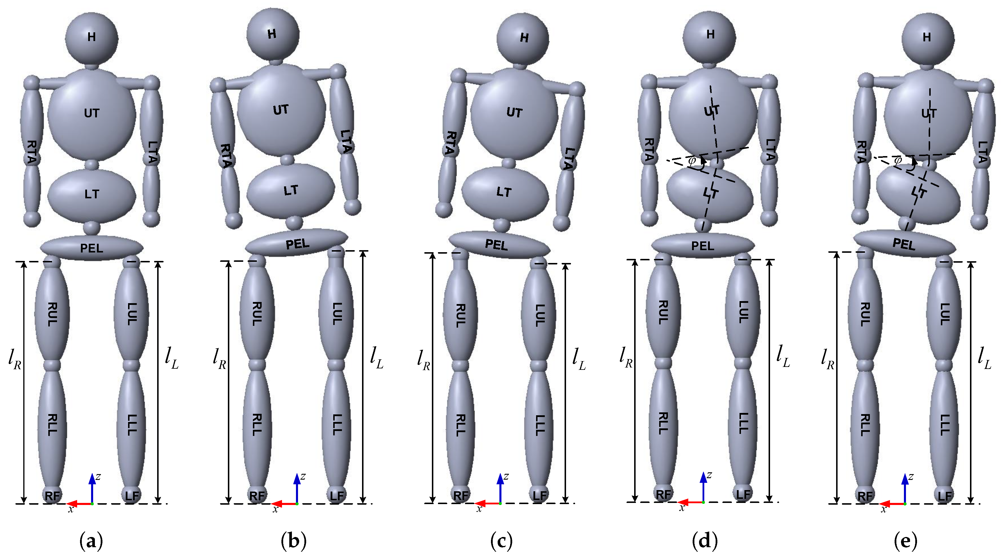
2.1. Anthropometric Human Body Model

An anthropometric human body model with variable leg length and scoliosis is shown in Figure 2. For the purpose of this research, LLD evaluation and compensation were done only for subjects with structural LLD (Figure 2b,c) and persons who developed scoliosis of the spine as a consequence of structural LLD (Figure 2e). The percentage of mass and the length of individual segments of the human body in Figure 2 are calculated according to [20,21].

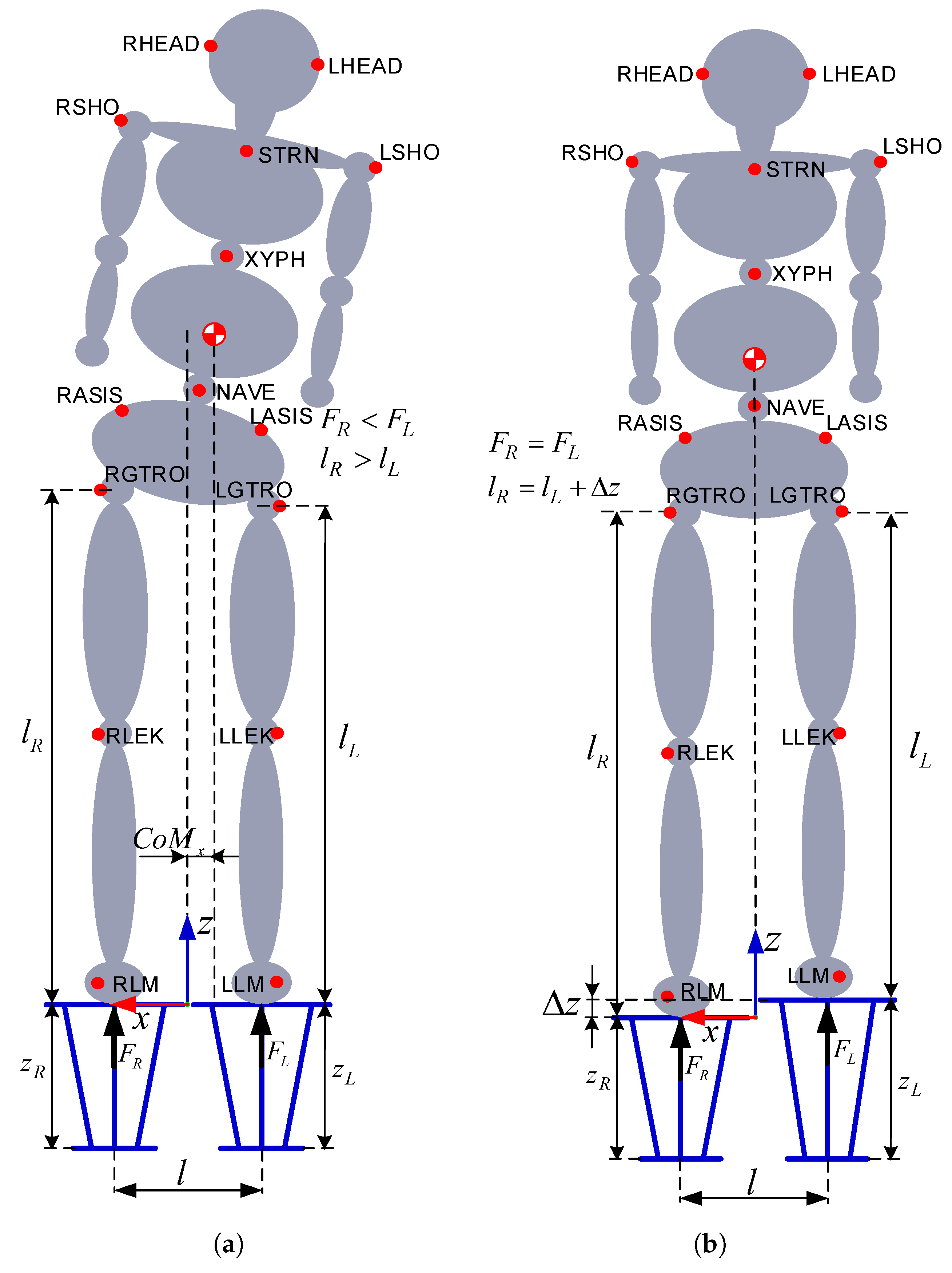
2.2. Human Body Balancing

Persons with LLD will have different load distribution on the two legs due to a shift in the body’s CoM [12,14]. The goal of compensating the length of the shorter leg is to ensure equal load distribution on both legs which can be achieved by human body balancing, that is, by moving the CoM to its expected position. The human body with structural LLD is shown in Figure 3a. The patient in Figure 3a would put more pressure on the force plate with his left leg than with his right ( F L > F R ). This is why a shift in the CoM toward the left leg can be detected, which implies that the right leg is longer than the left. Based on this analysis, it is necessary to lift the left force plate until the body’s CoM reaches its expected position (Figure 3b), that is, until both force plates register the same load ( F L = F R ). After this procedure, the human body will be balanced, and the height difference between the left and right force plate Δ z is the evaluation of LLD.
As already mentioned, this LLD estimation is used to help create orthopedic shoe insoles which equalize the load on the left and right legs. After making such insoles, the patient can repeat the CoM shift measuring procedure to see the influence of the shoe insoles on the load distribution on the patient’s legs. Additional help in the estimation of the patient’s status can be provided by markers located in previously defined anatomical positions. With these markers, many factors can be detected, such as scoliosis, knee flexion, as well as the position of the pelvis and shoulders, all of which influence the quality of the interpretation of results obtained when measuring the human body’s CoM.

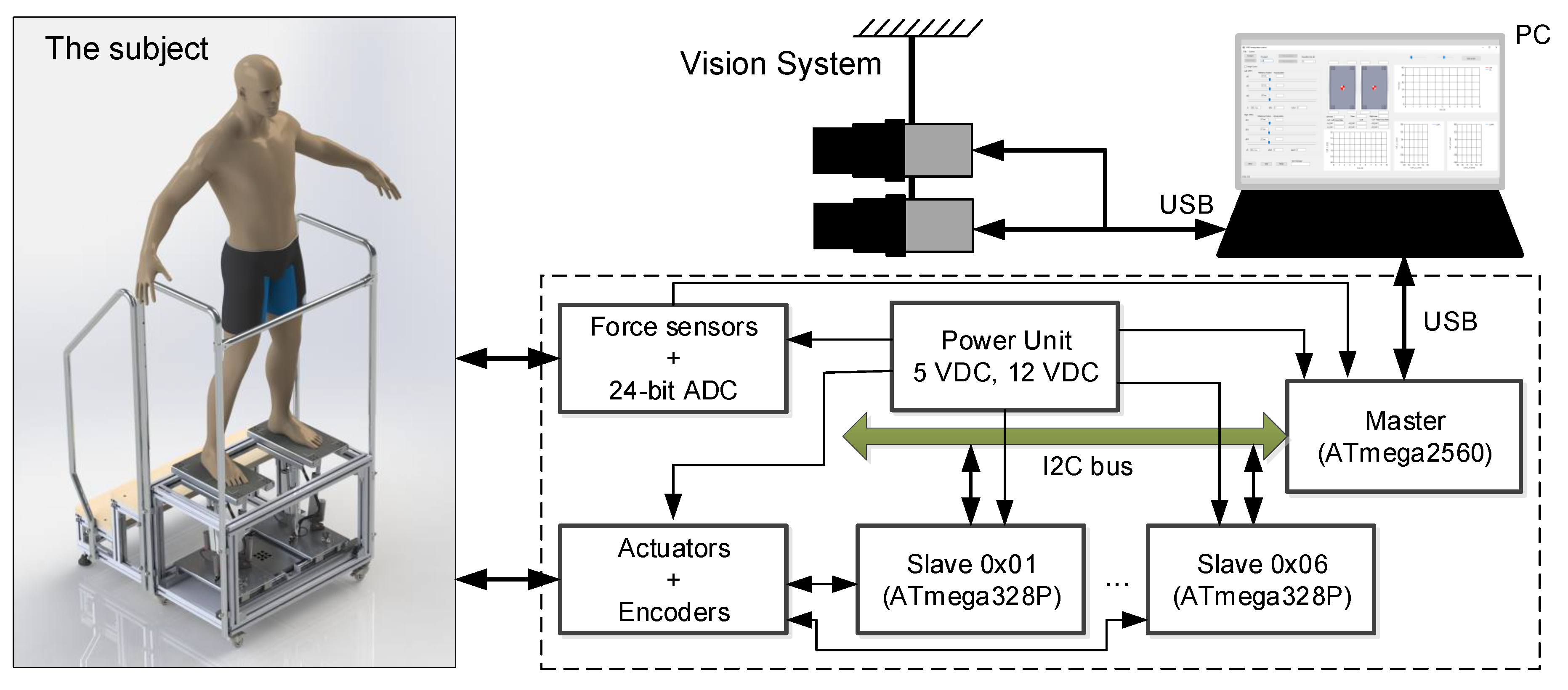
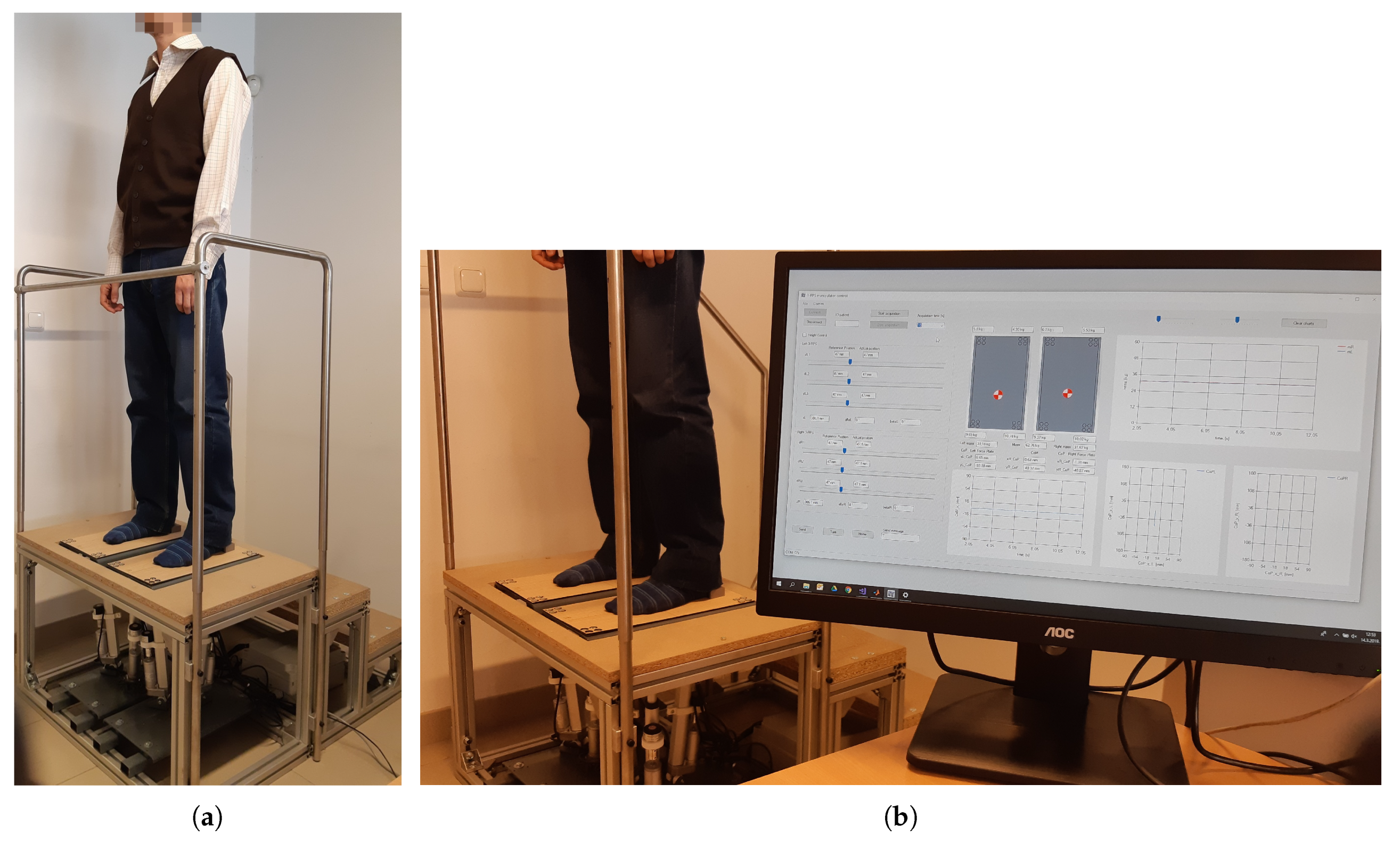
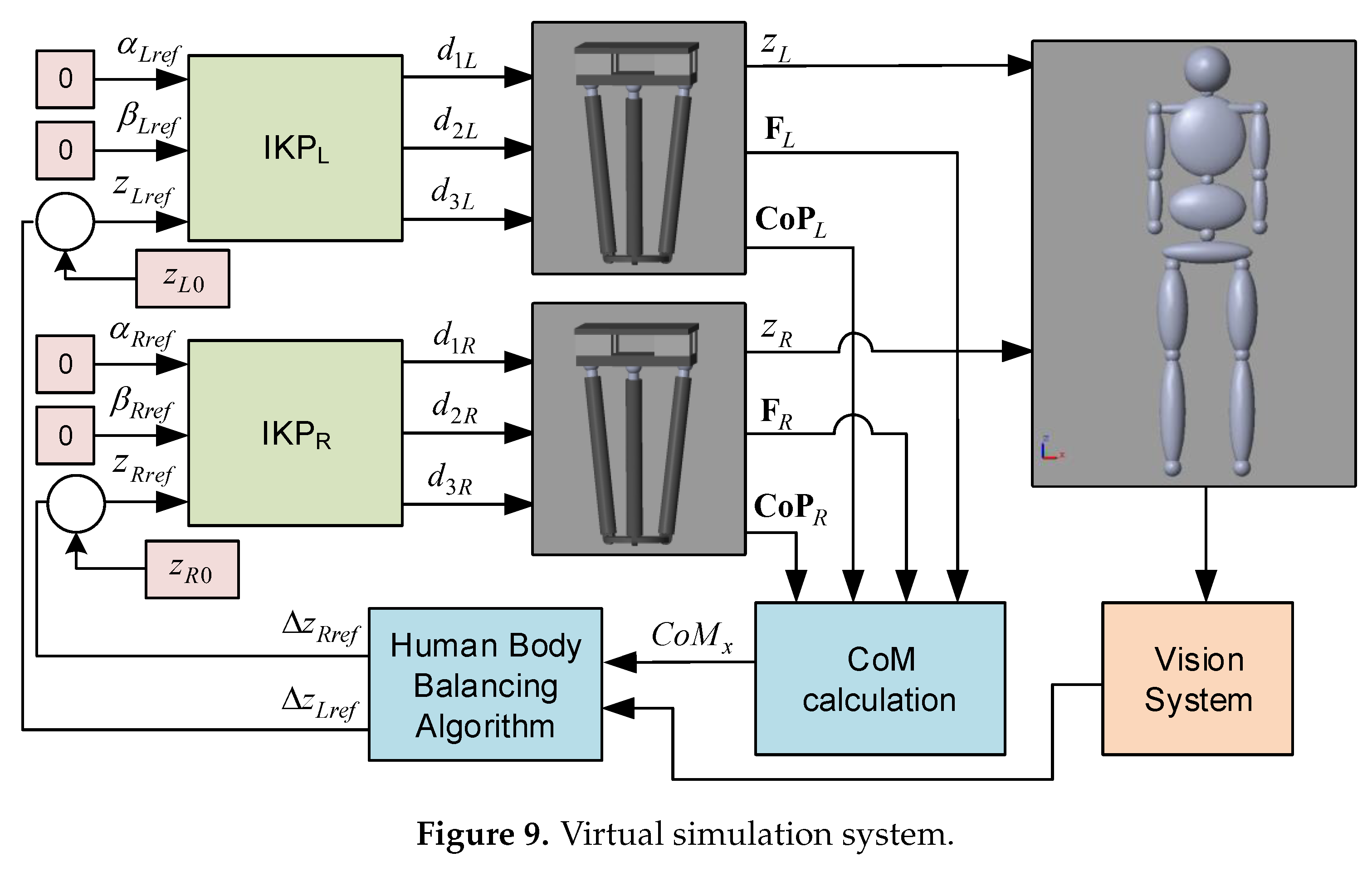
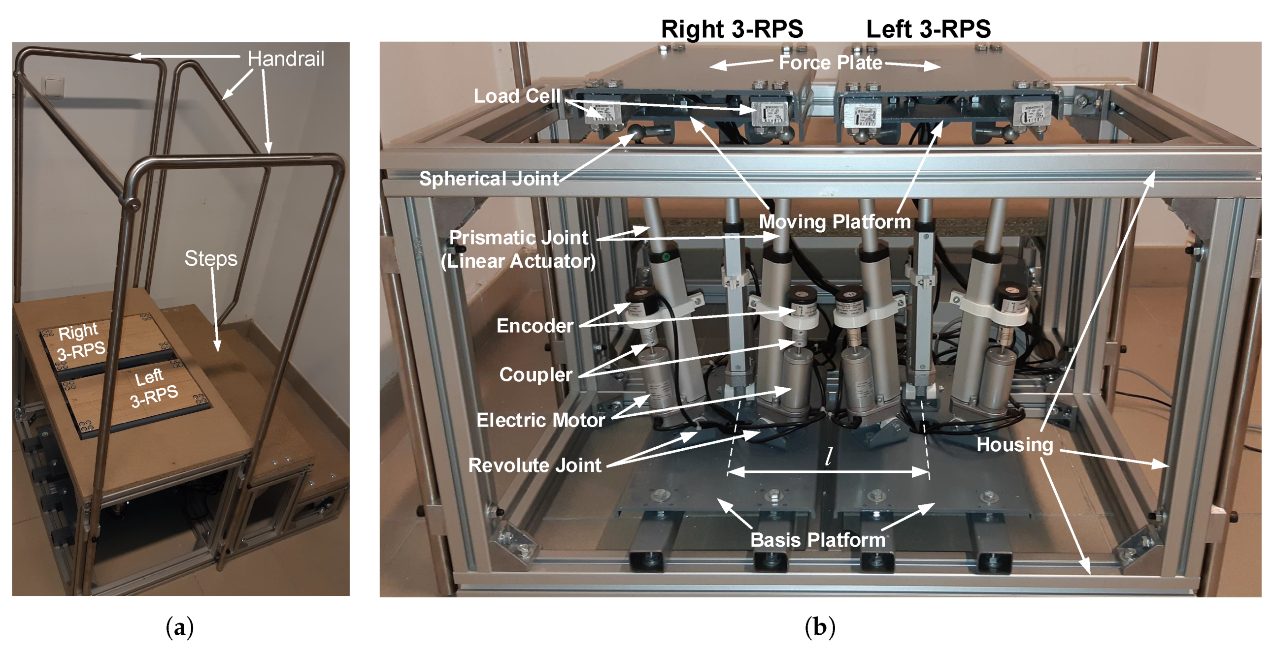
2.3. System Description

With the goal of evaluating and compensating LLD through human body balancing, the system shown in Figure 4 was proposed. A system defined in this way offers more possibility for leveling the pelvis by using RASIS and LASIS markers, as it changes the height of the platforms a person is standing on, which is a significant technical improvement of the standing on blocks measuring method [8,9]. It should be mentioned that the system’s force plates also have adjustable height and angles so that excessive pronation and supination can also be corrected in future studies.
The basic elements of the system shown in Figure 4 are as follows:
  • a mechanical set of two 3-RPS parallel manipulators with mobile force plates;
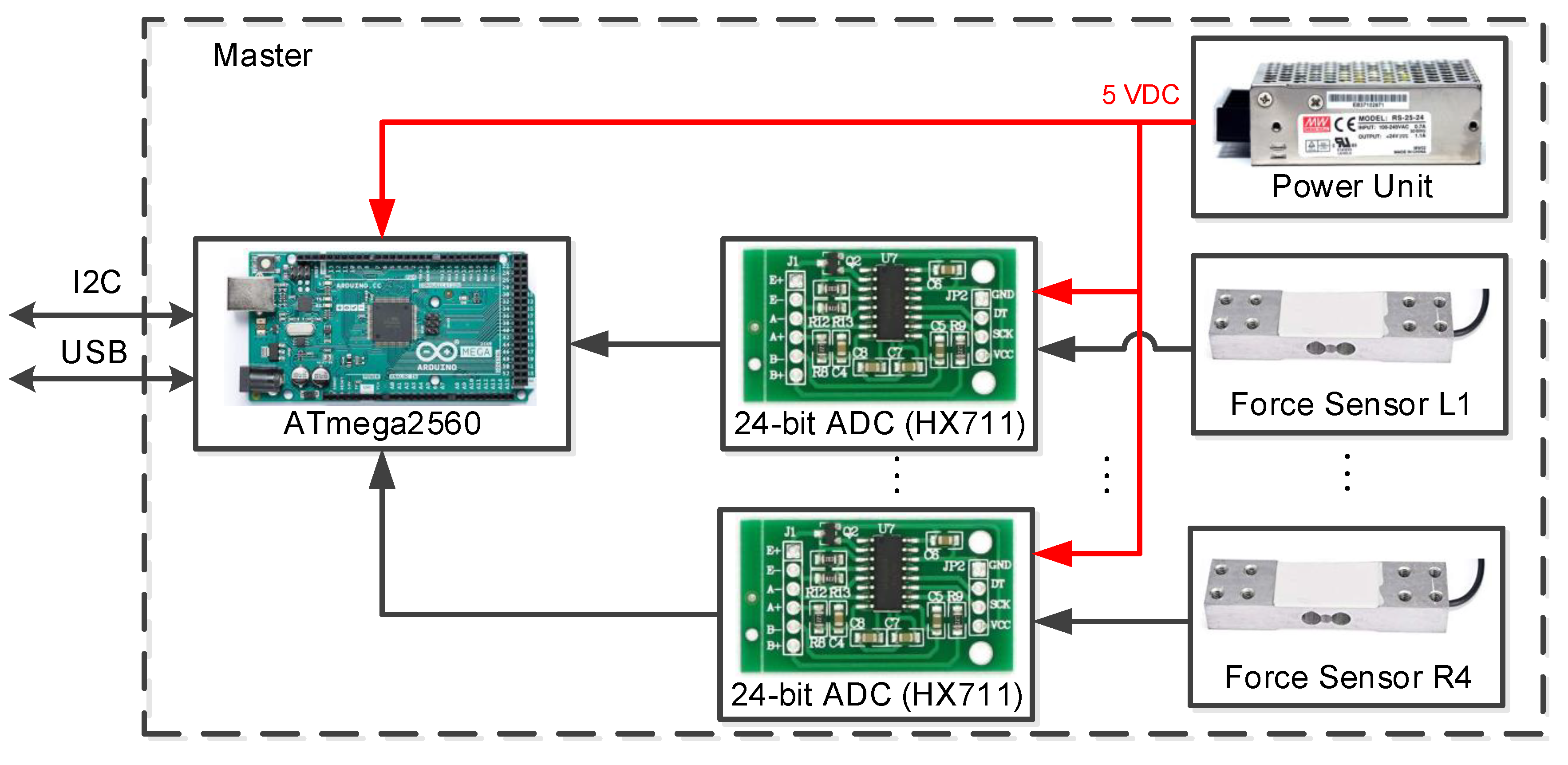
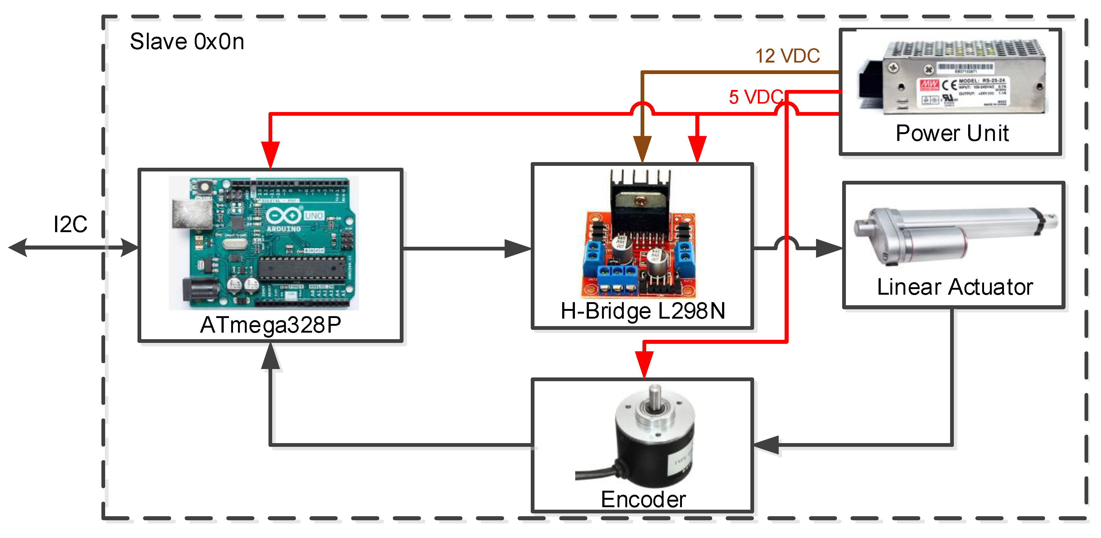
  • an electronic system for control, measuring and communication with the PC;
  • a vision system with two cameras; and
  • a PC application used for control and data collection.
A prototype of the mechanical set is shown in Figure 5a. It consists of two 3-RPS parallel manipulators mounted into the housing. The following prerequisites need to be fulfilled when choosing a manipulator from Figure 5a: small size, ability to manipulate high loads, lightweight, high accuracy and adjustable force plate height and angles. These requirements are met by 3-RPS parallel manipulators, which is why they were chosen for this system [22,23]. Force plates are added to the 3-RPS parallel manipulator’s moving platforms to determine the CoP of each leg and the CoM of the human body in the transverse plane.
The electronic system for control, measuring and communication with the PC consists of one master device and six slave devices. The slave devices control the length of the electronic linear actuators, that is, the height and angle of the 3-RPS parallel manipulators. The master device processes the forces measured on the force plates and communicates with the slave devices and the PC.
The vision system with two cameras films the person standing on the force plates, having one camera to record the person in the frontal plane and the other one in the sagittal plane. As mentioned above, the cameras use markers to follow specific anatomical positions and to give the diagnostician information on the correct posture of the human body.
The PC application makes it possible to adjust the height and angles of each 3-RPS parallel manipulator as necessary, and it also collects the data on the forces measured by the force plates. The collected data are shown in a graphic format and logged in a textual file for further processing. Figure 5b shows the application being used as the patient is standing on the moving force plates.

3. Mathematical Model of the System

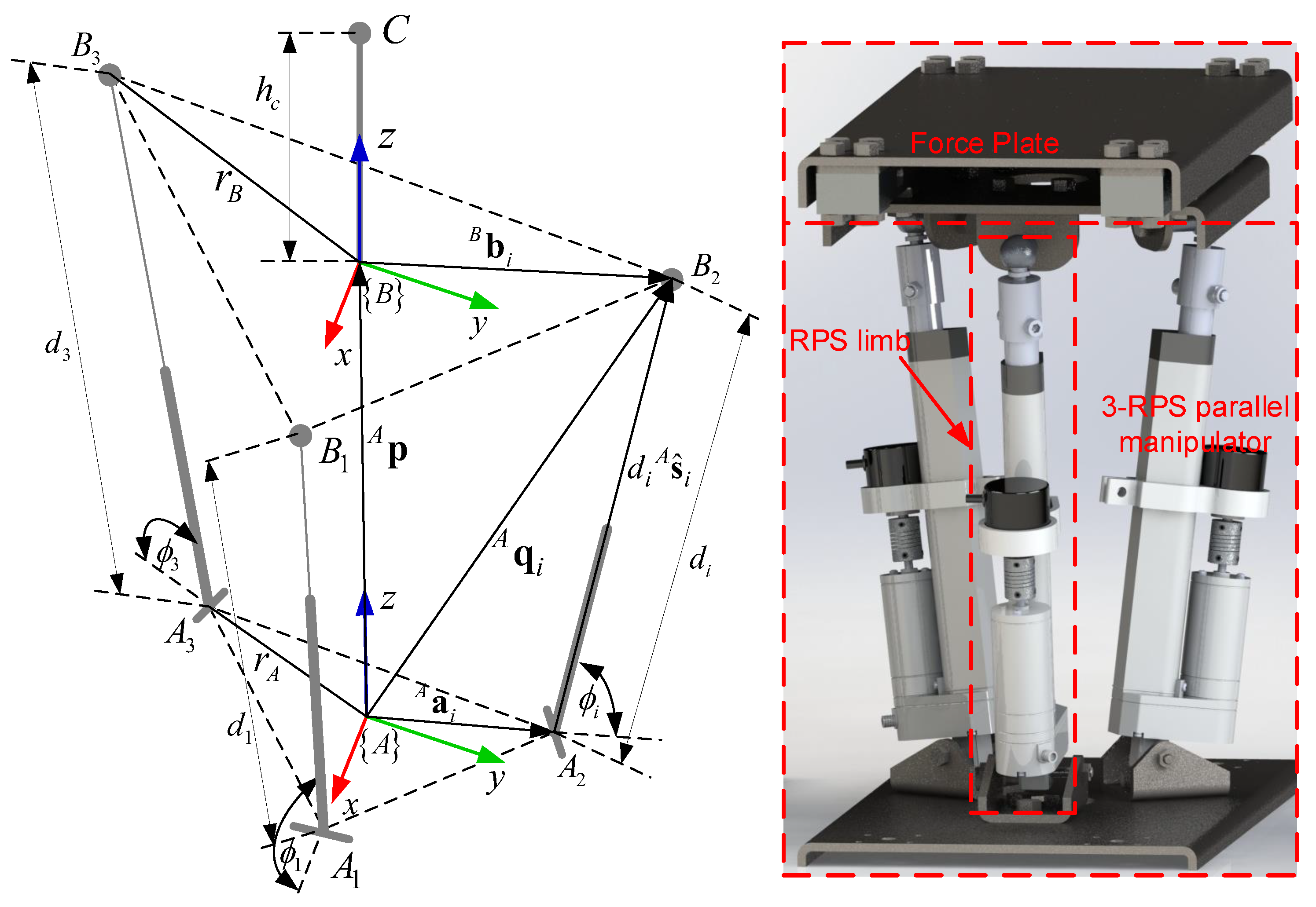
3.1. The Geometry of the 3-RPS Parallel Manipulator

The geometry of the 3-RPS parallel manipulator is shown in Figure 6. The 3-RPS parallel manipulator consists of a basis platform {A} and moving platform {B} which are connected to each other with three identical RPS limbs (Figure 6). The revolute joints (R) are connected with the basis platform in the vertices of the equilateral triangle A 1 A 2 A 3 . The prismatic joints (P) are linear actuators which change the length of the RPS limb d i , ( i = 1 , 2 , 3 ). Spherical joints (S) are connected to the moving platform in the vertices of the equilateral triangle B 1 B 2 B 3 . By changing the length of an RPS limb, the position and orientation of the 3-RPS parallel manipulator’s moving platform is also changed [24]. A force plate with the height h c is placed at the top of the moving platform.

3.2. Inverse Kinematic of the 3-RPS Parallel Manipulator

The 3-RPS parallel manipulator has three degrees of freedom (3-DOF). The solution to the inverse kinematic problem (IKP) for the 3-RPS parallel manipulator is the length of the linear actuators d i for a set position and orientation ( α , β , z) of the moving platform. According to Figure 6, the closed loop equation for each individual linear actuator length d i (i = 1, 2, 3) can be defined as [22,25]:
d i A s ^ i = A p + A R B B b i A a i
where
  • A s ^ i is the unit vector of the prismatic joint;
  • A p is the position vector of the moving platform center in the frame {A};
  • A R B is the rotation matrix of the moving frame {B} with respect to the frame {A};
  • B b i is the position vectors of spherical joints in the frame {B}; and
  • A a i is the position vectors of revolute joints in the frame {A}.
The length of the prismatic joint actuators can also be defined as a scalar product of Equation (1) with itself. The position vectors of revolute joints A a i ( i = 1 , 2 , 3 ) in the frame {A} are:
A a 1 = r A 0 0 , A a 2 = 1 2 r A 3 2 r A 0 , A a 3 = 1 2 r A 3 2 r A 0
where r A is the radius of the circumscribed circle of the equilateral triangle A 1 A 2 A 3 . Position vectors of spherical joints B b i ( i = 1 , 2 , 3 ) in the frame {B} are:
B b 1 = r B 0 0 , B b 2 = 1 2 r B 3 2 r B 0 , B b 3 = 1 2 r B 3 2 r B 0
where r B is the radius of the circumscribed circle of the equilateral triangle B 1 B 2 B 3 . The rotation matrix A R B of the moving frame {B} with respect to the frame {A} is as follows:
A R B = u x v x w x u y v y w y u z v z w z
A detailed presentation of the IKP of a 3-RPS parallel manipulator is given in [18]. The position vector of the center of the force plate B c in the frame {B} is:
B c = 0 0 h c T
The position vector of the center of the force plate A c in the frame {A} is:
A c = A p + A R B B c
The IKP for the left ( j = L ) and right ( j = R ) 3-RPS parallel manipulators is defined as follows:
d 1 j d 1 j d 1 j T = IKP j α j , β j , z j
where α j is the rotation of the force plate j around the x-axis, β j is the rotation of the force plate around the y-axis and z j is the position of the force plate on the z-axis.

3.3. Forward Kinematics of the 3-RPS Parallel Manipulator
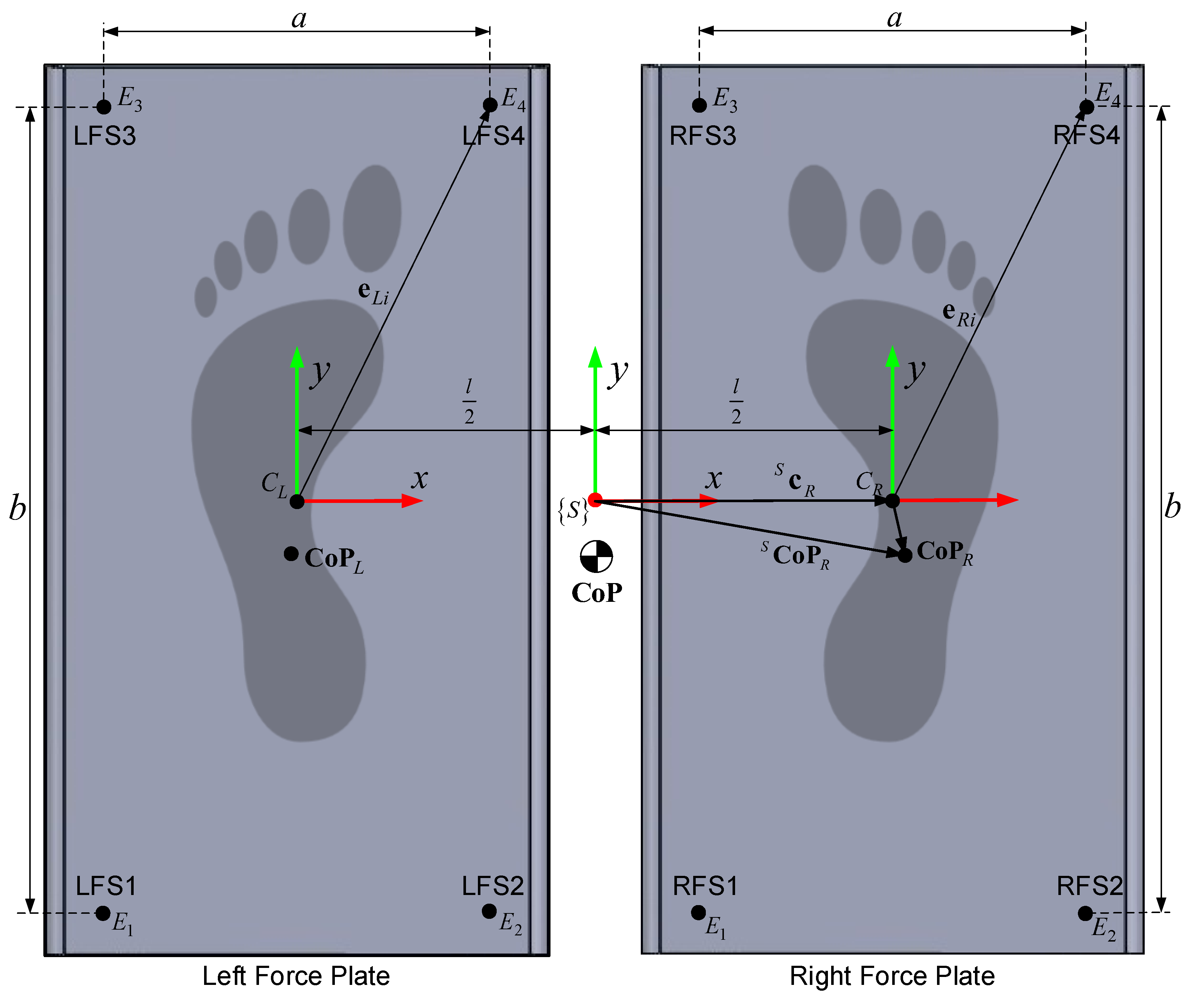
The solution to the forward kinematic problem (FKP) for the 3-RPS parallel manipulator can be found by determining the position and orientation ( α , β , z) of the moving platform for given lengths of linear actuators d i . In accordance with Figure 6, the position of spherical joints in the frame {A} can be described as follows:
A q 1 = r A + d 1 cos ϕ 1 0 d 1 sin ϕ 1 , A q 2 = r A 2 d 2 cos ϕ 2 2 3 r A + d 2 cos ϕ 2 2 d 2 sin ϕ 2 , A q 3 = r A 2 d 3 cos ϕ 3 2 3 r A + d 3 cos ϕ 3 2 d 3 sin ϕ 3
which gives the distance between the vertices of the equilateral triangle B 1 B 2 B 3 [26,27]:
B 1 B 2 = 3 r B A q 1 A q 2 = 3 r B B 2 B 3 = 3 r B A q 2 A q 3 = 3 r B B 3 B 1 = 3 r B A q 3 A q 1 = 3 r B
By squaring and rewriting Equation (9) in implicit form, a system of nonlinear equations is created. The solution to the system of nonlinear equations are unknown angles ϕ 1 , ϕ 2 and ϕ 3 with which the positions of spherical joints can be calculated. By substituting the angles ϕ 1 , ϕ 2 and ϕ 3 into Equation (8), the position vector of the center of the moving platform A p in the frame {A} can be found with the following expression:
A p = A q 1 + A q 2 + A q 3 / 3
The position of the force plate can be found by substituting Equation (10) into Equation (6) while the orientation of the moving platform can be determined with the following expression [26]:
α = atan 2 ( v z / cos β , w z / cos β ) β = sin 1 u z γ = atan 2 ( u y / cos β , u x / cos β )
where u x , u y , u z , v z and w z are elements of the rotation matrix A R B .

3.4. Force Plates

The study of a human body’s ability to maintain balance is often related to the CoP and CoM. While the CoP is a point defined in two dimensions and can be directly calculated with the help of force plates [28], the CoM is a point in three-dimensional space, and for the purposes of this paper, a projection of the CoM in the transverse plane is observed. As explained above, to calculate the CoP and CoM, two force plates, one per left and right leg, are used, each comprising force sensors (Figure 7).
The left and right legs’ CoPs are shown in the local frame of the left and right force plates. The parameters for force measuring in Figure 7 are:
  • a is the distance between the sensors along the x-axis;
  • b is the distance between the sensors along the y-axis; and
  • l is the distance between the origins of the left and right local force plate frame.
In the local force plate frame, the CoP is defined with the following equation [29,30]:
CoP j = C o P j x C o P j y = 1 i = 1 4 F j i i = 1 4 e j i F j i
In Equation (12), F j i ( j = L , R ; i = 1 , 2 , 3 , 4 ) is the force of each individual force plate sensor, whereas e j i is the position vector of each individual force plate sensor, which can be expressed in the left ( j = L ) or right ( j = R ) force plate frame as:
e j 1 = a 2 b 2 , e j 2 = a 2 b 2 , e j 3 = a 2 b 2 , e j 4 = a 2 b 2
The coordinates of the left ( j = L ) and right ( j = R ) force plates’ CoPs in the frame {S} can be expressed with the following equations:
S Co P j = Co P j + S c j ,
while, at the same time, the position vectors of the left and right force plate centers in the frame {S} are:
S c L = l 2 0 T , S c R = l 2 0 T
The CoP of the human body can be defined with the CoP of the left and right legs as follows:
CoP = S Co P L i = 1 4 F L i + S Co P R i = 1 4 F R i i = 1 4 F L i + i = 1 4 F R i
With an ideally static posture of the human body, the CoM projection in the transverse plane is in the same point as the CoP. However, due to the human body swaying, there will be a deviation between the CoM and CoP. Hence, when standing still, instead of equality, the CoM of the human body in the transverse plane is approximated with the CoP [28]:
CoM = C o M x C o M y CoP

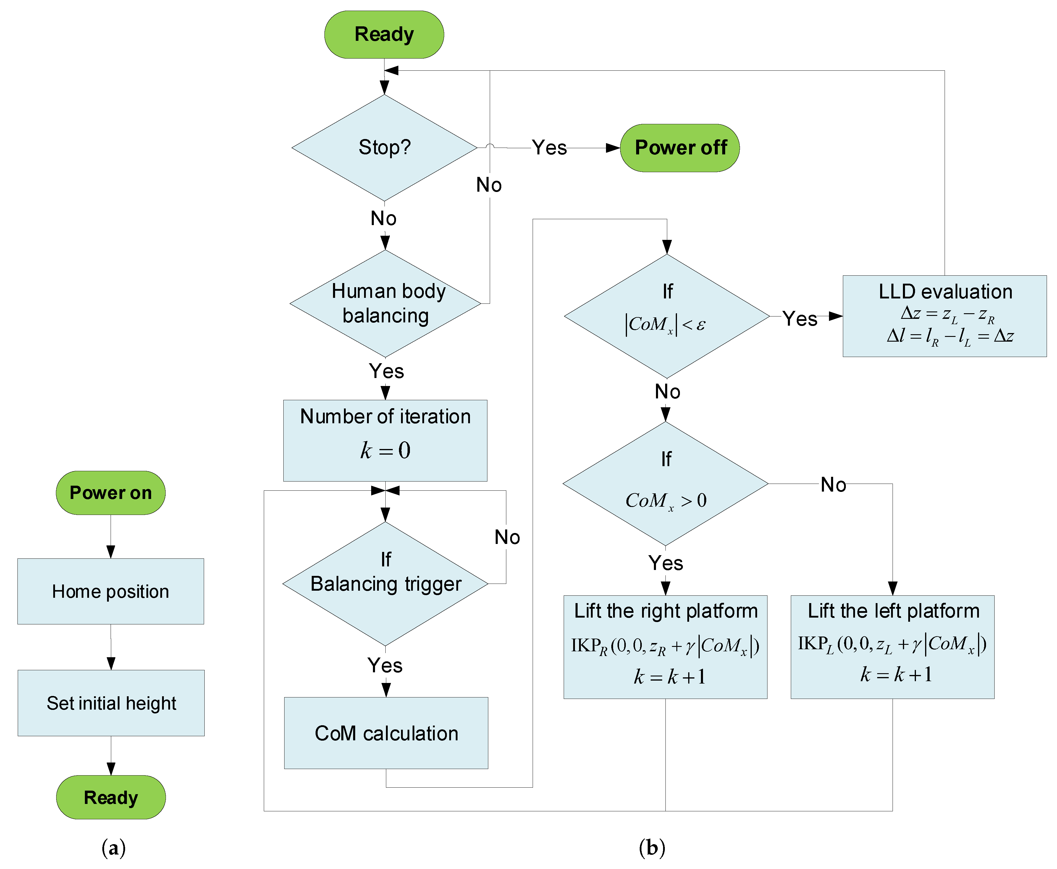
4. Human Body Balancing Algorithm

As stated in the Introduction, the LLD evaluation is done by balancing the human body. For this purpose, the Human Body Balancing Algorithm has been developed, the goal of which is to bring the human body’s CoM to the expected position ( C o M x = 0 ) in the frame {S}, as shown in Figure 7. Initial tests of subject behavior on moving force plates showed that changing the force plates’ height causes the subject’s CoM to move in unexpected manners. If standard controllers were used for human body balancing, the aforementioned shift in the human body’s CoM could cause unpredictable behavior when adjusting the height of the 3-RPS parallel manipulators’ moving platforms. This is why an iterative process of human body balancing was made, as shown in Figure 8b. Before running the HBBA, it is necessary to turn the system on and set the 3-RPS parallel manipulators to the same initial height (Figure 8a). After reaching the initial height of the 3-RPS parallel manipulators, the system is in its ready state, which is a precondition to run the HBBA (Figure 8b).
A subject climbs the steps to the force plates and places their feet on marked locations with the help of a diagnostician. When the subject is standing on the force plates, the Human Body Balancing starts and the number of iterations k of the HBBA is set to 0. The diagnostician asks the subject to be still, relaxed and to maintain a naturally upright posture. If a static and naturally relaxed posture is achieved, the algorithm initiates the balancing trigger. The human body’s CoM is calculated based on the relation in Equation (17). If C o M x ε , one of the moving platforms of the 3-RPS parallel manipulators will be lifted. The amount the right ( j = R ) or left ( j = L ) platform will rise equals to:
Δ z j r e f = γ C o M x
The weight variable γ is an adaptive constant (refer to γ in Section 5.4.2). After lifting the left or right moving platform, the subject resumes their static and relaxed posture and naturally upright stance, after which the procedure is repeated (Figure 8b). The algorithm stops the human body balancing if the following is valid:
C o M x < ε
where ε is an acceptable deviation from the human body’s CoM along the x-axis in comparison to the expected position C o M x = 0 . When the condition defined in Equation (19) is fulfilled, the height difference between the left and right force plate is measured:
Δ z = z L z R
which finally gives the LLD evaluation as:
Δ l = l R l L = Δ z

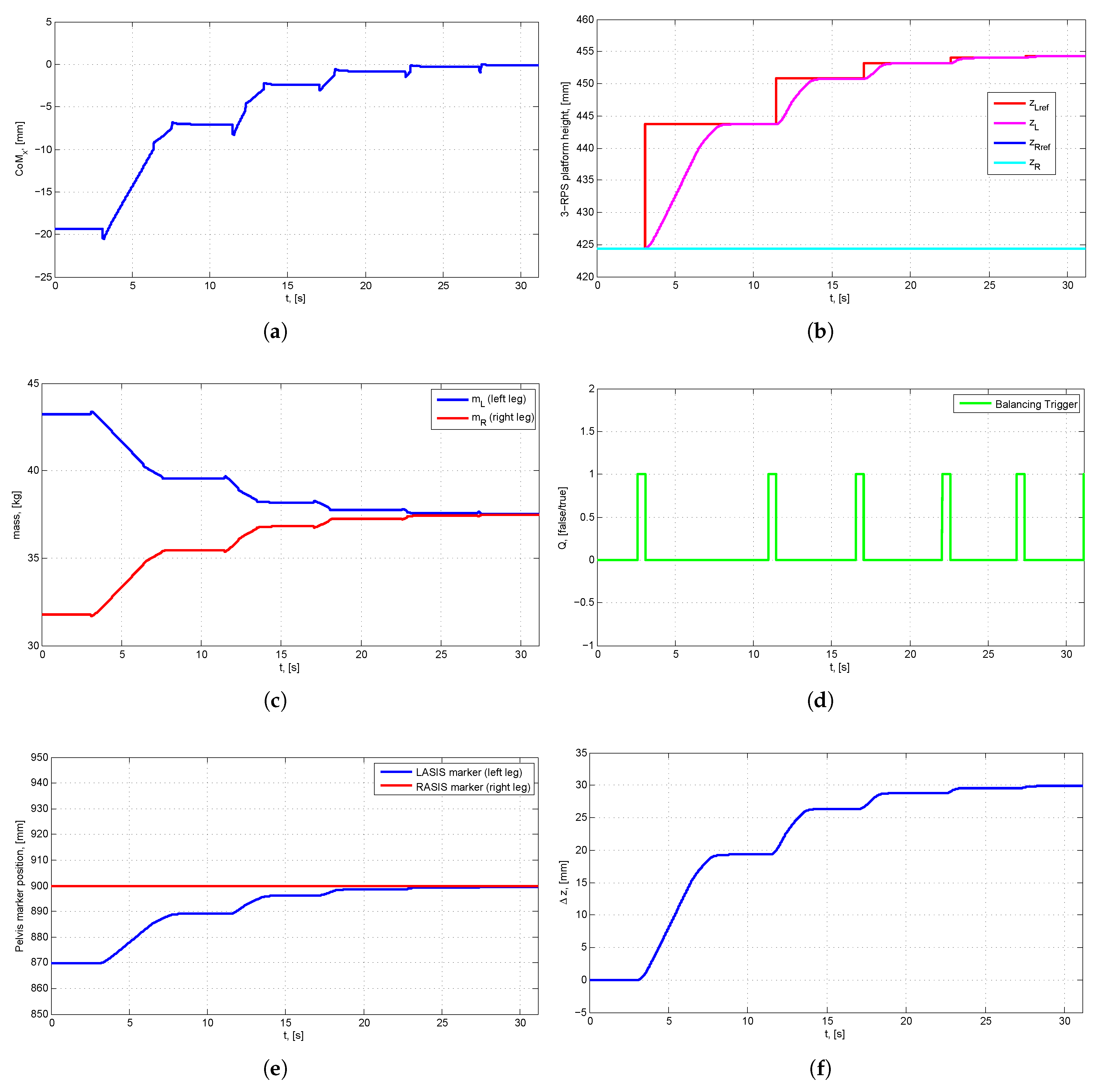
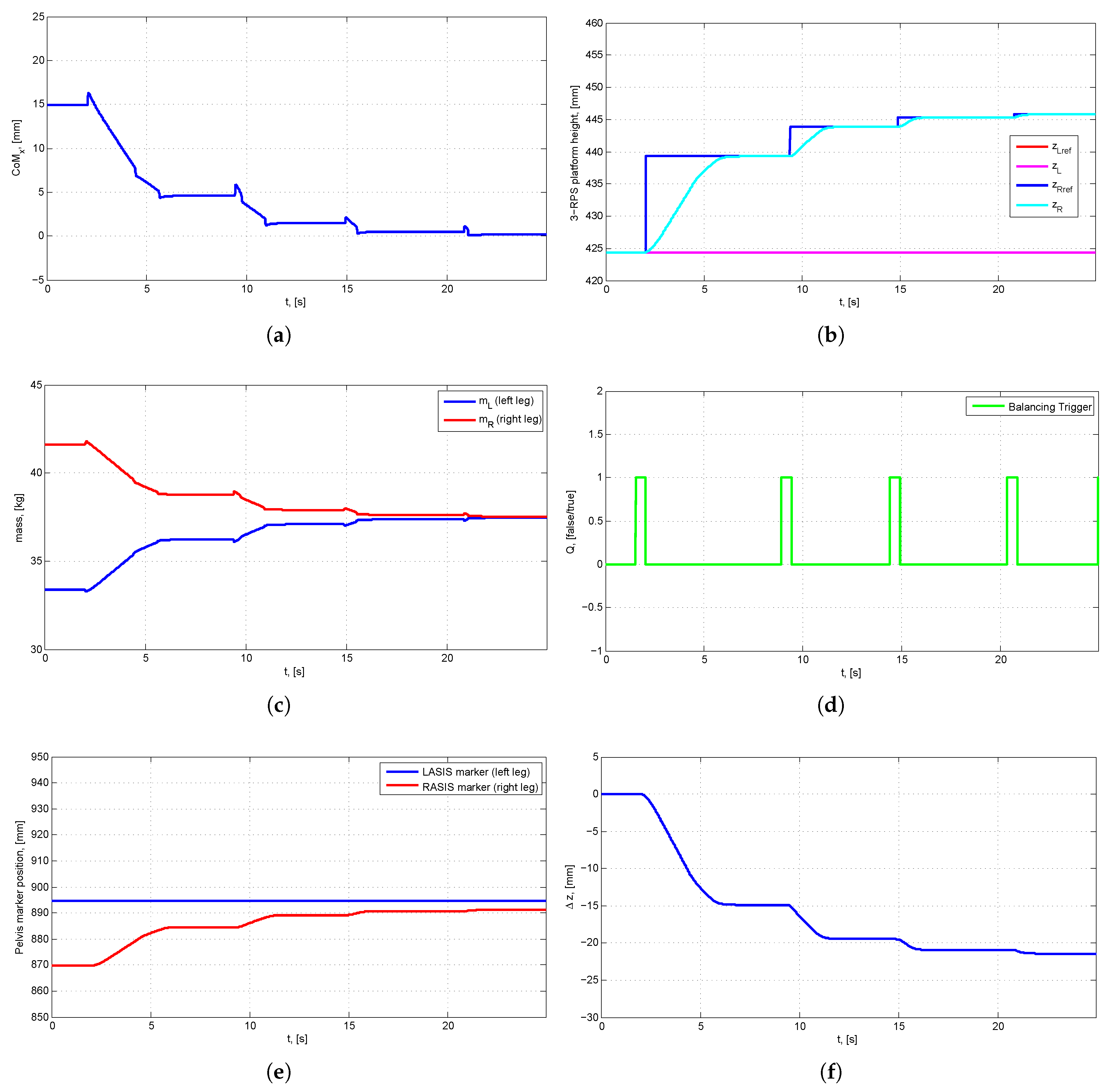
4.1. Simulation Results

To test the new LLD evaluation and compensation methodology using the HBBA, a virtual simulation model was made in MATLAB/Simulink®, as shown in Figure 9 (the model is available for download at [31]). The model of the 3-RPS parallel manipulators and the anthropometric model of the human body standing on force plates were both made with the use of SimMechanics ToolBox. The IKP L and IKP R blocks calculate the reference lengths of the 3-RPS parallel manipulators’ linear actuators with Equation (7). The virtual models of the 3-RPS parallel manipulators with moving force plates calculate the FKP and CoP for the left and the right leg. The HBBA was realized with a state machine and according to the flowchart shown in Figure 8b. The positions of the markers used in the simulation are shown in Figure 3, and they were measured on specifically defined points of the human body virtual model.
Herein, we present two typical scenarios for LLD evaluation and compensation with the help of the HBBA. In the first scenario, the human body has LLD, whereas, in the second, the human body has both LLD and scoliosis.

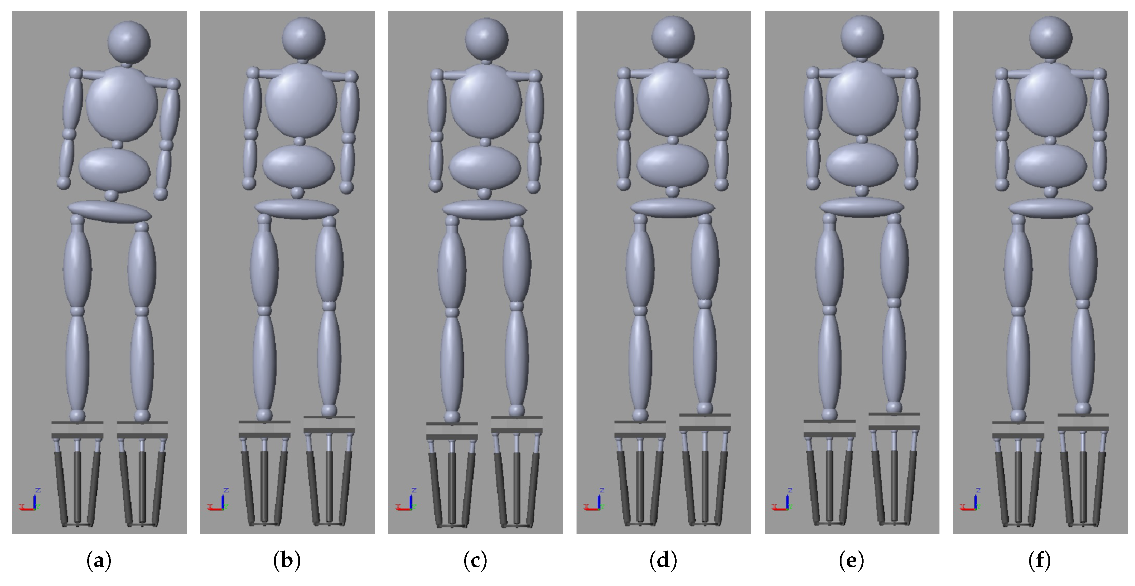
4.1.1. Scenario 1: Human Body with LLD

The mass and height of the human body in Scenario 1 are 75 kg and 175 cm. The length difference between the right and left leg is Δ l = 30 mm, and the scoliosis angle is ϕ = 0 . The HBBA parameters are ε = 0.2 mm and γ = 1 . The initial height of the left and right force plates is 424.4 mm. The HBBA in Scenario 1 finished after five iterations, as shown in Figure 10. At the beginning of the simulation, the human body model, presented face-in, was leaning toward the left (shorter) leg (Figure 10a), and in the final HBBA iteration, the human body model is balanced (Figure 10f).
In the initial state ( k = 0 ), the C o M x is −19.35 mm, which is the result of a bigger load on the left force plate ( m L = 43.22 kg) than the load on the right force plate ( m R = 31.78 kg). The position of the LASIS marker along the z-axis equals to 869.8 mm, and the position of the RASIS marker along the z-axis is 899.8 mm. The positions of the LASIS and RASIS markers, as well as the position of the CoM along the x-axis, point out to the patient having LLD. The markers STRN, XYPH and NAVE lie on the same line, which points to the fact that patient has no scoliosis.
Considering that the | C o M x | ε , according to the algorithm in Figure 8b and Equation (18), the left platform will be lifted by 19.35 mm. The responses of the variables monitored during the runtime of the HBBA are shown in Figure 11. The values of these variables at the end of each iteration are shown in Table 1. The HBBA, according to Table 1, gradually reduces the CoM’s deviation along the x-axis by lifting the left force plate with the 3-RPS parallel manipulator. Every new calculation of the C o M x for the purpose of adjusting the force plate height will be done following the rising edge of the balancing trigger signal shown in Figure 11d that is generated when the human body on the force plate is static. At every change of the force plate’s height, there is a trough in the C o M x (Figure 11a). This is due to the increased force which the left leg is applying on the force plate following the acceleration of the manipulator.
The HBBA stops when in the final iteration ( k = 5 ) the C o M x amounts to −0.09 mm. The height of the left force plate z L is 454.31 mm, and the height of the left force plate z R is 424.4 mm. The difference in load of the left ( m L = 37.53 kg) and right ( m R = 37.47 kg) legs on their respective force plate is 0.06 kg, which points to the balance of the human body being achieved. The location of the LASIS marker along the z-axis is 899.7 mm, and the position of the RASIS marker along the z-axis is 899.8 mm. The difference in the markers’ height is 0.1 mm, which denotes that the pelvis is level. According to Equation (20), the difference in height between the left and right force plate Δ z is 29.91 mm. The LLD evaluation based on Equation (21) is Δ l = 29.91 mm, which following Equation (21) means that the right leg is longer than the left leg by 29.91 mm, while the simulated height difference between the left and right leg equaled to 30 mm. The precision of the HBBA will depend on the defined deviation ε . By lowering the deviation ε , the number of the HBBA’s iteration increases, which can prolong the LLD evaluation and make the real-world subject feel restless. It should be mentioned that. if the human body model has only LLD, the HBBA will reach the same results as the LLD measuring method standing on blocks [8], but much more quickly and completely automatically.

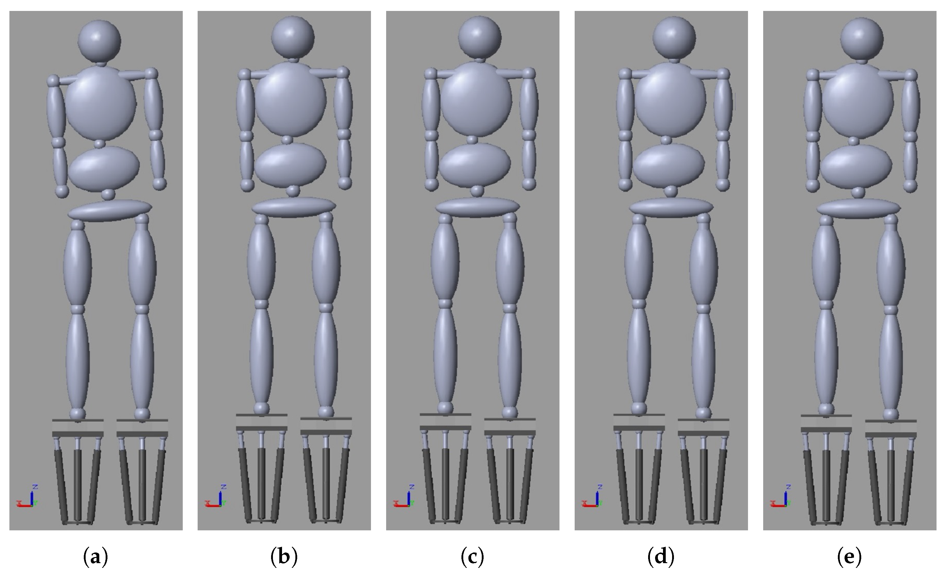
4.1.2. Scenario 2: Human Body with LLD and Scoliosis

The mass and height of the human body in Scenario 2 are 75 kg and 175 cm. The length difference between the left and right legs is Δ l = −25 mm, and the scoliosis angle is ϕ = 11 . The HBBA parameters are ε = 0.2 mm and γ = 1 . The initial height of the left and right force plate is 424.4 mm. The HBBA in Scenario 2 was finished after four iterations, as shown in Figure 12. At the beginning of the simulation, the human body model was leaning toward the right (shorter) leg (Figure 12a), and the lumbar spine was leaning toward the left (longer) leg [32]. The final HBBA iteration is shown in Figure 12e. Considering that the goal of human body balancing is load symmetry on the left and right leg, the human body with LLD and scoliosis will not have a level pelvis in the final step, as was the case in Scenario 1.
In the initial state ( k = 0 ), the C o M x is 14.88 mm, which is a consequence of the higher load on the right force plate ( m R = 41.61 kg) than the load on the left force plate ( m L = 33.39 kg). The location of the LASIS marker along the z-axis is 894.8 mm, and the position of the RASIS marker along the z-axis is 869.8 mm. The positions of the RASIS and LASIS markers, as well as the CoM position along the x-axis, point to the patient having LLD. The STRN and XYPH markers lie on the line p 1 , and the XYPH and NAVE markers lie on the line p 2 . The angle between the lines p 1 and p 2 is 169 , showing that the subject has scoliosis, the angle of the scoliosis being ϕ = 11 . Considering that | C o M x | ε , according to the algorithm in Figure 8 and Equation (18), the right platform should be lifted by 14.88 mm. The responses of the variables monitored during the runtime of the HBBA is shown in Figure 13. The values of the variables at the end of each iteration are shown in Table 2. According to Table 2, the HBBA gradually reduces the deviation of the CoM along the x-axis by lifting the right force plate with the 3-RPS parallel manipulator.
The HBBA stops when in the final iteration ( k = 4 ) the C o M x equals to 0.17 mm. The height of the left force plate z L is 424.4 mm, and the height of the right force plate z R is 445.83 mm. The load difference between the left ( m L = 37.46 kg) and the right ( m R = 37.54 kg) legs on their respective force plates equals to 0.08 kg, which shows that the human body is balanced. The location of the LASIS marker along the z-axis is 894.8 mm, and the location of the RASIS marker along the z-axis is 891.2 mm. The difference in marker height is 3.6 mm, which denotes that the pelvis is not level. The height difference between the left and right force plate is Δ z = −21.43 mm which gives Δ l = −21.43 mm. The simulated difference in leg length was 25 mm, meaning that the LLD evaluation gained via the HBBA is not equal to the real-world LLD because the subject has scoliosis. The goal of the HBBA is to achieve a symmetrical load on the left and right leg, which was achieved, as shown in Figure 13c. A symmetrical load on the left and right legs will be achieved if an orthopedic shoe insole is made for the patient with an elevation of 21.43 mm under the right leg.

5. Mechatronic System Design

Driven by very promising results obtained in the simulation, to confirm our hypothesis on real patients, we built a mechatronic system that is described in this section.

5.1. Mechanical Design

Elements of the mechanical set with two 3-RPS parallel manipulators with moving force plates are shown in Figure 14.
Two identical 3-RPS parallel manipulators with moving force plates are mounted onto a housing with the following dimensions: 900 × 550 × 580 mm. The distance between the left and right 3-RPS parallel manipulators is l = 265 mm. The steps and handrail on the mechanical system (Figure 14a) are used by the patient to safely and securely stand on the force plates.
Parts of 3-RPS parallel manipulators with moving force plates are shown in Figure 14b. The revolute joints, mounted onto the basis platform, are geometrically located in the vertices of an equilateral triangle with an incircle radius of r A = 60 mm.
Three linear actuators (prismatic joints) connected to the revolute joints are driven by a DC electric motor with a nominal voltage of 12 VDC. The maximum speed of the linear actuators is 5.7 mms 1 , and the maximum thrust force of the linear actuators is 1500 N. The minimal length of the linear actuator is 308.7 mm, and its maximal length is 458.7 mm. There is an incremental encoder attached to the body of the linear actuator. The spherical joints that connect the linear actuators to the moving platforms and are geometrically located in the vertices of an equilateral triangle with an incircle radius of r B = 100 mm. A force plate mounted onto the moving platform comprises four force sensors that are geometrically located in the vertices of a rectangle with the dimensions a = 168 mm × b = 361 mm.

5.2. Electronic Design

The electronic part of the system is used to control the position of the linear actuators, to measure force with the force sensors and to communicate with the PC running the control and data collection application. The electronic architecture of the system consists of one master device (Figure 15) and six slave devices (Figure 16).

5.2.1. Master Device

The master device consists of an ATmega2560 microcontroller, eight analog-to-digital (ADC) HX711 converters, eight force sensors and a power unit. The force sensors are calibrated with etalon weights weighing 100 g, 200 g, 500 g and 1000 g prior to use [33]. The master device sends the slave devices a reference position of the linear actuators and at the same time communicates to the PC the current positions of the linear actuators and force sensor measurements.

5.2.2. Slave Device

The slave device consists of an ATmega328P microcontroller, linear actuator, L298N motor driver, incremental encoder and power unit. The L298N motor driver and incremental encoder are used to control the position of the linear actuators, thus changing the height and angle of the moving platform. The resolution of the incremental encoder is 360 impulses per revolution, providing very precise positioning of the linear actuators.

5.3. Software Design

5.3.1. Firmware for Microcontrollers

The software used for the master and slave devices was written in the C++ programming language and the integrated development platform Amtel Studio 7.0. When the system is booted, the master device sends a request to the slave devices to set the 3-RPS parallel manipulators into their home position set to 355.7 mm. After that, the slave devices wait for instructions from the master device on moving the 3-RPS parallel manipulators into a new position and orientation. A precisely-defined data frame (eight measurements from the force sensors and six current positions of the linear actuators) is sent to the PC every 100 ms, while the PC asynchronously sends data (the reference positions of the linear actuators) to the master device.

5.3.2. PC Application for Control and Data Collection

The graphic user interface (GUI) of the PC application for control and data collection is shown in Figure 17. It was made in the .NET Framework and C# programming language. The application can be used to set the reference positions of linear actuators or the position and orientation of the force plates on the moving platforms of the 3-RPS parallel manipulator. Data measured by the force sensors and the current position of the linear actuators are shown through the GUI, as well as the CoP of the left and right legs, the human body’s CoM and the mass measured by the force plate under the left and the right legs. When a person is standing on the force plates, the process of collecting data with the application can start, with an acquisition time frame of 10–60 s. When the acquisition time is out, the application automatically saves a textual file with logged data about force sensor measurements and the positions of the linear actuators, as well as the responses on the left and right leg CoP, the human body’s CoM, and load on the left and right legs. By further processing the collected data, more detailed analyses can be made. The HBBA is implemented into the application and it is used to evaluate a patient’s LLD, as described above.

5.3.3. Vision System

The vision system consists of two GigE Vision industrial cameras and 15 IR markers located in various positions on the human body, as shown in Figure 3. Image processing from both cameras is done in the programming language C++. Through the markers, the diagnostician receives information about the posture of the human body, knee flexion and LLD based on the height difference between the left and right side of the pelvis (LASIS and RASIS markers). Considering that even persons without LLD can have different loads on the left and right legs, information about the height of the left and right sides of the pelvis is crucial for conducting tests. The minimal marker resolution in this vision system is 1 mm, and the accuracy of the LASIS and RASIS marker height measurements depends on correctly placing the markers in reference anatomical locations of the human body.

5.4. Experimental Results

5.4.1. Experiment 1: Healthy Population—Left and Right Leg Load Distribution

The first experiment’s goal was to test the new mechatronic system on the healthy population and to confirm the findings in [1], where it was concluded that people without LLD can also have asymmetrically distributed loads on their left and right legs. The experiment included 46 volunteers (23 women + 23 men). The study was conducted in accordance with the Declaration of Helsinki, and the protocol was approved by the Ethics Committee of the Bjelovar University of Applied Sciences. The average volunteer age was 22.18 years (SD = 5.52 years). The criteria for exclusion from this group of volunteers were having LLD, scoliosis, incorrect posture, diabetes and Body Mass Index (BMI) > 30 [1].
In the first experiment, the volunteers’ loads on their left and right legs were measured, as well as the position of the CoM ( C o M x ). Under the researchers’ supervision, the volunteers placed their left and right feet on specifically marked locations on the force plates. The distance between the volunteers’ heels was 24 cm. The left and right force plates were set to the same height of 424.4 mm. The researcher gave the volunteers the instruction to maintain a naturally upright posture and to face forward. For every volunteer, the loads on their left and right legs were measured and the CoM along the x-axis ( C o M x ) was found. This was done in 10 s with the application shown in Figure 17. With the help of a tailor’s tape measure, the heights of the volunteers’ LASIS and RASIS anatomical points were measured as compared to the basis. The BMI was calculated as the ratio of mass and squared height of the human body. The mean value, standard deviation and minimum and maximum of the conducted measurements are shown in Table 3. According to statistical results in Table 3, there is an asymmetry in the load on the left and right legs of healthy volunteers, which coincides with the research findings in [1].
Load measurements of the left and right legs and the CoM along the x-axis ( C o M x ) for three chosen volunteers are shown in Figure 18 and Table 4. Volunteer 1 has a higher load on the right leg (Figure 18a) and a shift in the CoM along the x-axis higher than 0 (Figure 18b). Volunteer 2 has a higher load on the left leg (Figure 18c) and a shift in the CoM along the x-axis lower than 0 (Figure 18d). Volunteer 3 has approximately the same load on both the left and right legs (Figure 18e) and a shift in the CoM along the x-axis approximately equal to 0 (Figure 18f). The standard deviation of the C o M x variable according to Table 4 is lower than 1 mm for all volunteers, pointing to a static posture. This confirmed the presumption that the projection of the human body’s CoM in the transverse plane lies in the same point as the CoP [28].
Volunteers 1 and 2, although they are not diagnosed with LLD, have an asymmetrical load distribution on the left and right legs. This is why it is also necessary to include a vision system in the process of evaluation and compensation of LLD, as it will provide information on the LASIS and RASIS marker heights, as well as answer the question if the subject has scoliosis.

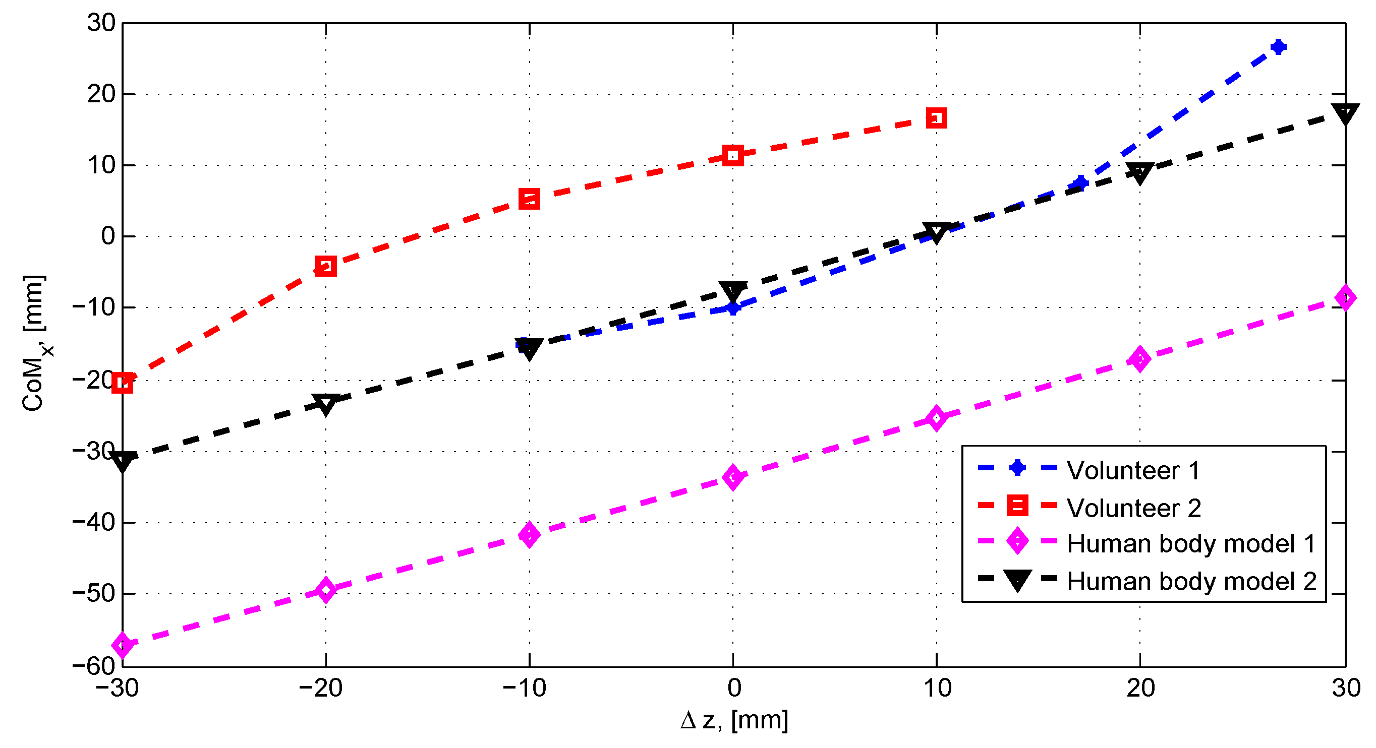
5.4.2. Experiment 2: Shift in the CoM Caused by a Force Plate Height Difference Shift

While conducting these experiments, it was noticed that the relation between the shift in height difference ( Δ z ) and corresponding change in the CoM varied with the BMI, mass and posture of a patient. That is why two separate experiments were done with two volunteers and compared with simulations for two different human body models. The results are shown in Figure 19. It can be seen that, in all cases, increasing the height difference between the force plates Δ z also increases the CoM shift along the x-axis ( C o M x ). However, functions that relate the CoM to Δ z are not the same. For example, in the case of Volunteer 1, the function is convex, while for Volunteer 2 it is concave. This observation can be well-used when creating an adaptation algorithm of the weight variable γ in Equation (18), which would reduce the number of iterations of the HBBA and make LLD measurement a more pleasant experience for the patient. In the future, we plan to continue investigating in that direction by conducting measurements on more subjects in order to receive more relevant data and finally develop an adaptive algorithm for the variable γ .

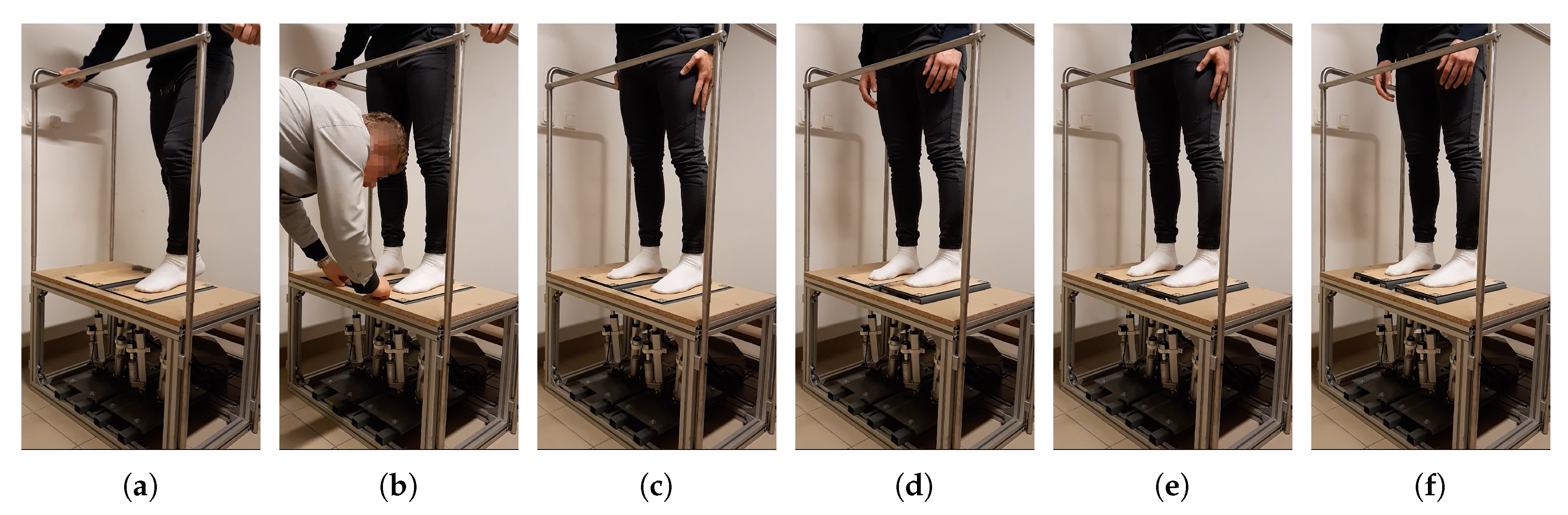
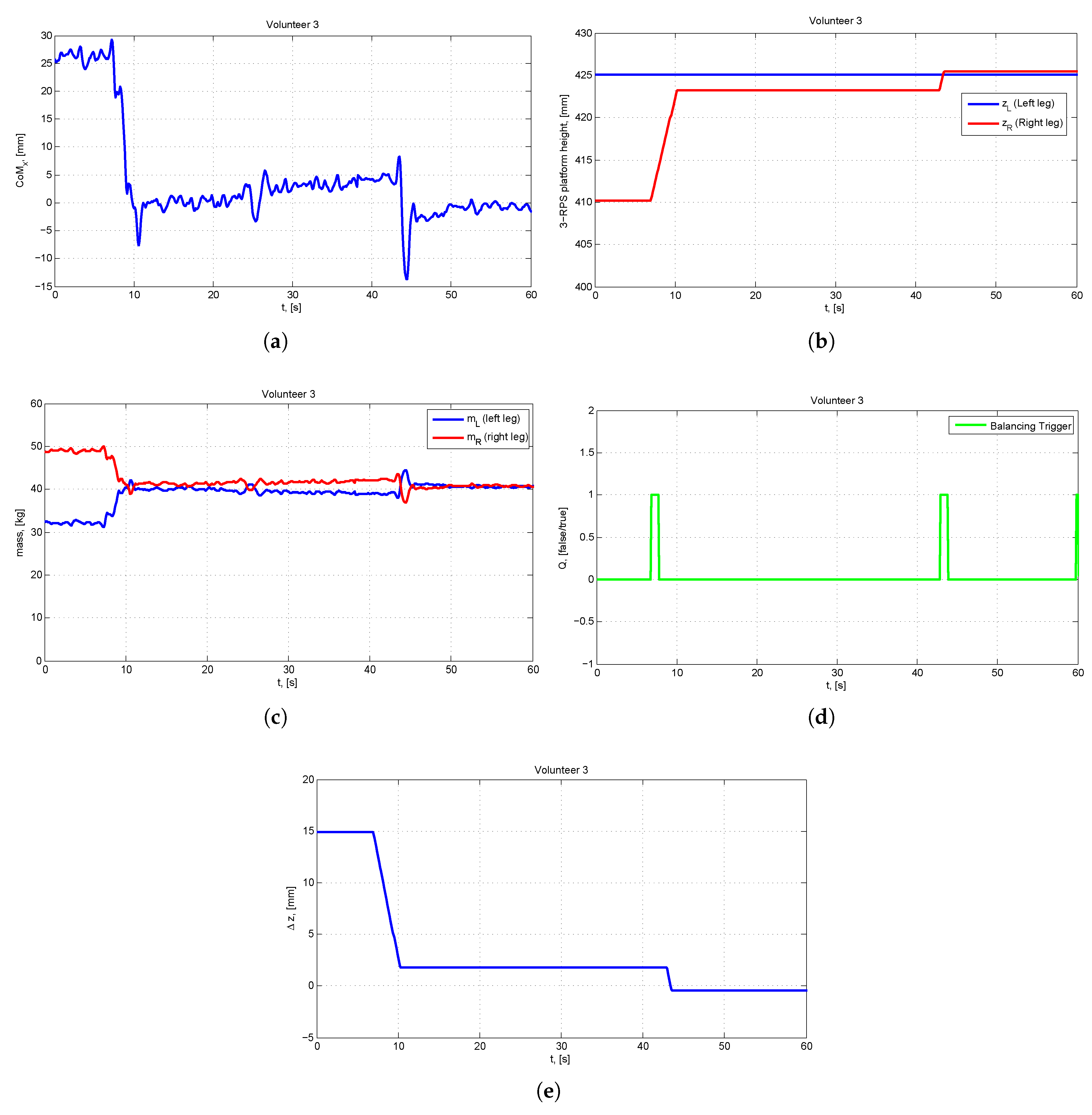
5.4.3. Experiment 3: A Healthy Volunteer with a Simulated LLD

The goal of Experiment 3 was to test the HBBA algorithm on a volunteer with a simulated LLD. The mass and height of the volunteer in Experiment 3 are 81.14 kg and 179 cm. As can be seen in Figure 18e and Table 4, Volunteer 3 has approximately equal loads on both legs, as well as the same positions of the LASIS and RASIS markers. The placement of Volunteer 3 on the force plates and the conducting of the LLD evaluation and compensation with a simulated LLD is shown in Figure 20. When Volunteer 3 stood still and had a static posture on the force plates, the height of which was 425 mm (Figure 20c), the system evaluated that Volunteer 3 is balanced.
The simulation of shortening the right leg was done by reducing the height of the right force plate z R from 425 mm to 410 mm (Figure 20d). This simulated length difference between the left and right legs equal to Δ l = −15 mm. The HBBA had the task of balancing Volunteer 3. The HBBA parameters were ε = 1 mm and γ = 0.5 . In the initial state ( k = 0 ), the C o M x equaled 26.5 mm, which was the result of a higher load on the right force plate ( m R = 48.98 kg) than on the left force plate ( m L = 32.16 kg). Considering that | C o M x | ε , according to the algorithm in Figure 8 and Equation (18), the right platform was lifted by 13.2 mm. The response of the variables observed while running the HBBA is shown in Figure 21.
The values of these variables at the end of each iteration are shown in Table 5. The first HBBA iteration was started at t = 6.7 s after the subject was maintaining a static and calm posture. After the first iteration, the load difference between the left and right leg was reduced. It is interesting to notice that at the time t = 25 s (Figure 21c), the subject lost their focus just as the new iteration of the HBBA was about to be run. The balancing trigger was not issued and the HBBA waited for the subject to once again maintain a static posture so that a new iteration was started at t = 43 s.
The HBBA stopped when in the last iteration ( k = 2 ) the C o M x equaled −0.6 mm. The height of the left force plate z L was 425.0 mm, and the height of the right force plate z R was 425.4 mm. The loads on the left and right legs were m L = 40.73 kg and m R = 40.46 kg, which shows that Volunteer 3 was balanced. The LLD was evaluated to −15.4 mm in this case, while the simulated LLD equaled to 15 mm. The HBBA successfully conducted an evaluation and compensation of simulated LLD for Volunteer 3.

6. Conclusions

In this paper, a new methodology for the Evaluation and Compensation of LLD for Human Body Balancing is presented. For this purpose, a mechatronic system with two 3-RPS parallel manipulators comprising moving force plates with adjustable height and angles was developed. The mathematical model of the system was described in detail and a virtual simulation model in Matlab was created. To balance the human body standing on the force plates, a novel algorithm (HBBA) was developed and tested on a virtual simulation model and the mechatronic system. Two simulation models, namely the human body model with LLD and scoliosis, are described in the paper and tested by simulation. In both cases, the HBBA achieved an equalization of leg load distribution.
To validate the new mechatronic system, leg load distribution measurements were conducted on 46 volunteers. The obtained results show that people without evident LLD have asymmetric load distribution on their legs. Thus, it is important to include a vision system in the process of estimating LLD so that measurements of the location of predefined anatomical points are taken into account for the final diagnosis. While conducting the experiments, it was noticed that the relation between the shift in height difference ( Δ z ) and corresponding change in the CoM varies with the BMI, mass and posture of a patient. This fact will be used in the future for the creation of an adaptation algorithm for the weight parameter of the HBBA.
Finally, the HBBA was tested on a volunteer with simulated LLD. It was experimentally shown that the HBBA compensated the volunteer’s simulated LLD and balanced their body. The developed mechatronic system enables the leveling of the pelvis by changing the height of the platforms a subject is standing on, which is a significant improvement in terms of the technical aspect, duration and patient experience when compared to the standing on blocks measuring method.
In future work, tests will be done with the HBBA on persons who have both LLD and scoliosis. Based on promising results, presented herein, we received funds under Proof-of-Concept program from Croatian agency HAMAG BICRO for clinical trials on 35 patients that already started and we hope to have clinical results in the next 18 months. Furthermore, the fact that the force plates’ angle can be altered opens up the possibility of creating an algorithm that can correct excessive pronation and supination. Additionally, the developed mechatronic system can be used for rehabilitation and therapeutic purposes, with the aim of working out the joints and thus helping a patient achieve the desired range of motion.

Supplementary Files

Supplementary File 1

Author Contributions

Conceptualization, Z.V., K.O., A.M., H.K. and S.B.; Formal analysis, Z.V., K.O., H.K. and S.B.; Methodology, Z.V. and S.B.; Project administration, J.N. and A.M.; Software, Z.V. and J.N.; Supervision, H.K. and S.B.; Validation, Z.V. and K.O.; Writing—original draft, Z.V. and S.B.; and Writing—review and editing, Z.V. and S.B.

Funding

This research was funded as part of the pre-seed capital program Proof of Concept (PoC) by HAMAG-BICRO, Croatia.

Conflicts of Interest

The authors declare no conflict of interest.

Abbreviations

The following abbreviations are used in this manuscript:
LLDLeg Length Discrepancy
CTComputerized Tomography
MRIMagnetic Resonance Imaging
ASISAnterior Inferior Iliac Spine
3-RPS3-Revolute-Prismatic-Spherical
CoMCenter of Mass
CoPCenter of Pressure
3-DOFThree Degrees of Freedom
IKPInverse Kinematic Problem
FKPForward Kinematic Problem
IRInfra-red
BMIBody Mass Index

References

  1. Eliks, M.; Ostiak-Tomaszewska, W.; Lisiński, P.; Koczewski, P. Does structural leg-length discrepancy affect postural control? Preliminary study. BMC Musculoskelet. Disord. 2017, 18, 346. [Google Scholar] [CrossRef] [PubMed]
  2. Azizan, N.A.; Basaruddin, K.S.; Salleh, A.F. The Effects of Leg Length Discrepancy on Stability and Kinematics-Kinetics Deviations: A Systematic Review. Appl. Bionics Biomech. 2018, 2018, 5156348. [Google Scholar] [CrossRef] [PubMed]
  3. Khamis, S.; Danino, B.; Springer, S.; Ovadia, D.; Carmeli, E. Detecting Anatomical Leg Length Discrepancy Using the Plug-in-Gait Model. Appl. Sci. 2017, 7, 926. [Google Scholar] [CrossRef]
  4. Khamis, S.; Danino, B.; Ovadia, D.; Carmeli, E. Correlation between Gait Asymmetry and Leg Length Discrepancy—What Is the Role of Clinical Abnormalities? Appl. Sci. 2018, 8, 1979. [Google Scholar] [CrossRef]
  5. Khamis, S.; Carmeli, E. The effect of simulated leg length discrepancy on lower limb biomechanics during gait. Gait Posture 2018, 61, 73–80. [Google Scholar] [CrossRef] [PubMed]
  6. Gurney, B. Leg length discrepancy. Gait Posture 2002, 15, 195–206. [Google Scholar] [CrossRef]
  7. Ali, A.; Walsh, M.; O’Brien, T.; Dimitrov, B.D. The importance of submalleolar deformity in determining leg length discrepancy. Surgeon 2014, 12, 20–205. [Google Scholar] [CrossRef]
  8. Sabharwal, S.; Kumar, A. Methods for Assessing Leg Length Discrepancy. Clin. Orthop. Relat. Res. 2008, 466, 2910–2922. [Google Scholar] [CrossRef] [Green Version]
  9. Hanada, E.; Kirby, R.; Mitchell, M.; Swuste, J. Measuring leg-length discrepancy by the “iliac crest palpation and book correction” method: Reliability and validity. Arch. Phys. Med. Rehabil. 2001, 82, 938–942. [Google Scholar] [CrossRef]
  10. Khamis, S.; Springer, S.; Ovadia, D.; Krimus, S.; Carmeli, E. Measuring Dynamic Leg Length during Normal Gait. Sensors 2018, 18, 4191. [Google Scholar] [CrossRef]
  11. O’Brien, D.S.; Kernohan, G.; Fitzpatrick, C.; Hill, J.; Beverland, D. Perception of Imposed Leg Length Inequality in Normal Subjects. HIP Int. 2010, 20, 505–511. [Google Scholar] [CrossRef] [PubMed]
  12. Azizan, N.A.; Basaruddin, K.S.; Salleh, A.F.; Sakeran, H.; Sulaiman, A.R.; Cheng, E.M. The Effect of Structural Leg Length Discrepancy on Vertical Ground Reaction Force and Spatial—Temporal Gait Parameter: A Pilot Study. J. Telecommun. Electron. Comput. Eng. 2018, 10, 111–114. [Google Scholar]
  13. White, S.C.; Gilchrist, L.A.; Wilk, B.E. Asymmetric Limb Loading with True or Simulated Leg-Length Differences. Clin. Orthop. Relat. Res. 2004, 421, 287–292. [Google Scholar] [CrossRef] [PubMed]
  14. Swaminathan, V.; Cartwright-Terry, M.; Moorehead, J.; Bowey, A.; Scott, S. The effect of leg length discrepancy upon load distribution in the static phase (standing). Gait Posture 2014, 40, 561–563. [Google Scholar] [CrossRef] [PubMed]
  15. Abu-Faraj, Z.; MM, A.A.; RA, A.D. Leg Length Discrepancy: A Study on In-Shoe Plantar Pressure Distribution. In Proceedings of the 8th International Conference on Biomedical Engineering and Informatics (BMEI), Shenyang, China, 14–16 October 2015; pp. 381–385. [Google Scholar] [CrossRef]
  16. Vrhovski, Z.; Markov, M.; Pavlic, T.; Obrovac, K.; Mutka, A.; Nižetić, J. Design of a Mechanical Assembly for the Dynamic Evaluation of Human Body Posture. In Proceedings of the 16th International Scientific Conference on Production Engineering (CIM2017), Zadar, Croatia, 8–10 June 2017; pp. 237–242. [Google Scholar]
  17. Design of a Mechanical Assembly for the Dynamic Evaluation of Human Body Posture. Available online: https://youtu.be/C-4RpSqBi90 (accessed on 5 April 2019).
  18. Vrhovski, Z.; Obrovac, K.; Mutka, A.; Bogdan, S. Design, modeling and control of a system for dynamic measuring of leg length discrepancy. In Proceedings of the 21st International Conference on System Theory, Control and Computing (ICSTCC), Sinaia, Romania, 19–21 October 2017; pp. 693–698. [Google Scholar] [CrossRef]
  19. Vrhovski, Z.; Benkek, G.; Mutka, A.; Obrovac, K.; Bogdan, S. System for Compensating for Leg Length Discrepancy Based on the Estimation of the Centre of Mass of a Human Body. In Proceedings of the 26th Mediterranean Conference on Control and Automation (MED), Zadar, Croatia, 19–22 June 2018; pp. 637–642. [Google Scholar] [CrossRef]
  20. Lafond, D.; Duarte, M.; Prince, F. Comparison of three methods to estimate the center of mass during balance assessment. J. Biomech. 2004, 37, 1421–1426. [Google Scholar] [CrossRef]
  21. Robertson, D.; Caldwell, G.E.; Hamill, J.; Kamen, G.; Whittlesey, S.N. Research Methods in Biomechanics, 2nd ed.; Human Kinetics Publishers: Champaign, IL, USA, 2013. [Google Scholar]
  22. Ruiz-Hidalgo, N.C.; Blanco-Ortega, A.; Abúndez-Pliego, A.; Colín-Ocampo, J.; Arias-Montiel, M. Design and Control of a Novel 3-DOF Parallel Robot. In Proceedings of the International Conference on Mechatronics, Electronics and Automotive Engineering (ICMEAE), Cuernavaca, Mexico, 22–25 November 2016; pp. 66–71. [Google Scholar] [CrossRef]
  23. Garcia Gonzalez, L.; Campos, A. Maximal Singularity-Free Orientation Subregions Associated with Initial Parallel Manipulator Configuration. Robotics 2018, 7, 57. [Google Scholar] [CrossRef]
  24. Schadlbauer, J.; Walter, D.; Husty, M. The 3-RPS parallel manipulator from an algebraic viewpoint. Mech. Mach. Theory 2014, 75, 161–176. [Google Scholar] [CrossRef]
  25. Taghirad, H.D. Parallel Robots: Mechanics and Control; CRC Press: Boca Raton, FL, USA, 2013; pp. 77–95. [Google Scholar]
  26. Rad, C.; Manic, M.; Bälan, R.; Stan, S. Real time evaluation of inverse kinematics for a 3-RPS medical parallel robot usind dSpace platform. In Proceedings of the 3rd International Conference on Human System Interaction, Rzeszow, Poland, 13–15 May 2010; pp. 48–53. [Google Scholar] [CrossRef]
  27. Lukanin, V. Inverse kinematics, forward kinematics and working space determination of 3DOF parallel manipulator with S-P-R joint structure. Period. Polytech. Mech. Eng. 2005, 49, 39–61. [Google Scholar]
  28. Cotton, S.; Vanoncini, M.; Fraisse, P.; Ramdani, N.; Demircan, E.; Murray, A.; Keller, T. Estimation of the centre of mass from motion capture and force plate recordings: A study on the elderly. Appl. Bionics Biomech. 2011, 8, 67–84. [Google Scholar] [CrossRef]
  29. Eguchi, R.; Takahashi, M. Validity of the Nintendo Wii Balance Board for kinetic gait analysis. Appl. Sci. 2018, 8, 285. [Google Scholar] [CrossRef]
  30. Huang, C.W.; Sue, P.D.; Abbod, M.; Jiang, B.; Shieh, J.S. Measuring Center of Pressure Signals to Quantify Human Balance Using Multivariate Multiscale Entropy by Designing a Force Platform. Sensors 2013, 13, 10151–10166. [Google Scholar] [CrossRef] [PubMed]
  31. Vrhovski, Z.; Bogdan, S. Virtual Simulation Model for Evaluation and Compensation of Leg Length Discrepancy for Human Body Balancing. Available online: https://www.researchgate.net/publication/333668115_Virtual_Simulation_Model_for_Evaluation_and_Compensation_of_Leg_Length_Discrepancy_for_Human_Body_Balancing (accessed on 6 June 2019).
  32. Sheha, E.D.; Steinhaus, M.E.; Kim, H.J.; Cunningham, M.E.; Fragomen, A.T.; Rozbruch, S.R. Leg-Length Discrepancy, Functional Scoliosis, and Low Back Pain. JBJS Rev. 2018, 6, 1–8. [Google Scholar] [CrossRef] [PubMed]
  33. Zhu, Y. Design and Validation of a Low-Cost Portable Device to Quantify Postural Stability. Sensors 2017, 17, 619. [Google Scholar] [CrossRef] [PubMed]
Figure 1. Measuring leg load distribution by using two equal commercial scales.
Applsci 09 02504 g001
Figure 2. 12-segment anthropometric human body model with variable leg length and scoliosis (RF, Right Foot; LF, Left Foot; RLL, Right Lower Leg; LLL, Left Lower Leg; RUL, Right Upper Leg; LUL, Left Upper Leg; PEL, Pelvis; LT, Lower Trunk; UT, Upper Trunk; H, Head; RTA, Right Total Arm; LTA, Left Total Arm). Left leg length is given as l L , right leg length is l R , and the angle of scoliosis is ϕ : (a) human body without LLD and scoliosis ( l R = l L , ϕ = 0 ); (b) human body with LLD ( l R < l L , ϕ = 0 ); (c) human body with LLD ( l R > l L , ϕ = 0 ); (d) human body with scoliosis ( l R = l L , ϕ > 0 ); and (e) human body with LLD and scoliosis ( l R > l L , ϕ > 0 ).
Applsci 09 02504 g002
Figure 3. Human Body Balancing: (a) human body with LLD ( C o M x < 0 ); and (b) balanced human body ( C o M x = 0 ).
Applsci 09 02504 g003
Figure 4. System for evaluation and compensation of leg ength discrepancy for human body balancing.
Applsci 09 02504 g004
Figure 5. Display of the mechanical set with two 3-RPS parallel manipulators with moving force plates: (a) with the patient on the force plates; and (b) with the application used to diagnose the load on each of the patient’s legs.
Applsci 09 02504 g005
Figure 6. Geometry of 3-RPS parallel manipulator.
Applsci 09 02504 g006
Figure 7. Left and right leg force plate frames.
Applsci 09 02504 g007
Figure 8. Flowchart: (a) Turning the system on and moving the 3-RPS parallel manipulators to their initial height; and (b) Human Body Balancing Algorithm.
Applsci 09 02504 g008
Figure 9. Virtual simulation system.
Applsci 09 02504 g009
Figure 10. Scenario 1: (a) Initial state of the human body with LLD (algorithm iteration k = 0); (b) algorithm iteration k = 1; (c) algorithm iteration k = 2; (d) algorithm iteration k = 3; (e) algorithm iteration k = 4; and (f) the human body is balanced (algorithm iteration k = 5).
Applsci 09 02504 g010
Figure 11. Scenario 1: (a) C o M x , the position of the human body’s CoM; (b) reference height of the left ( z L r e f ) and right ( z R r e f ) force plate, current height of the left ( z L ) and right ( z R ) force plate; (c) the load on the left ( m L ) and right ( m R ) leg; (d) the balancing trigger signal (Q) marking the start of a new HBBA iteration; (e) position of the LASIS and RASIS markers, which are located on the pelvis; and (f) left and right force plate height difference ( Δ z ), which corresponds with the LLD evaluation ( Δ l ) in the HBBA’s final step.
Applsci 09 02504 g011
Figure 12. Scenario 2: (a) Initial state of the human body with LLD and scoliosis (algorithm iteration k = 0); (b) algorithm iteration k = 1; (c) algorithm iteration k = 2; (d) algorithm iteration k = 3; and (e) the human body with LLD and scoliosis is balanced (algorithm iteration k = 4).
Applsci 09 02504 g012
Figure 13. Scenario 2: (a) C o M x , the position of the human body’s CoM; (b) reference height of the left ( z L r e f ) and right ( z R r e f ) force plate, current height of the left ( z L ) and right ( z R ) force plate; (c) the load on the left ( m L ) and right ( m R ) leg; (d) the balancing trigger signal (Q) marking the start of a new HBBA iteration; (e) position of the LASIS and RASIS markers, which are located on the pelvis; and (f) left and right force plate height difference ( Δ z ), which corresponds with the LLD evaluation ( Δ l ) in the HBBA’s final step.
Applsci 09 02504 g013
Figure 14. Parts of the mechanical set with two 3-RPS parallel manipulators with moving force plates: (a) handrail and steps of the mechanical set; and (b) left and right 3-RPS parallel manipulators with moving force plates.
Applsci 09 02504 g014
Figure 15. Electronic schematic of the master device.
Applsci 09 02504 g015
Figure 16. Electronic schematic of the slave device.
Applsci 09 02504 g016
Figure 17. PC application for control and data collection.
Applsci 09 02504 g017
Figure 18. Measurements of loads on the left m L and right m R legs and the CoM along the x-axis ( C o M x ) for three chosen volunteers: (a) Volunteer 1, the loads on the left m L and the right m R legs; (b) Volunteer 1, CoM along the x-axis ( C o M x ); (c) Volunteer 2, the loads on the left m L and the right m R legs; (d) Volunteer 2, CoM along the x-axis ( C o M x ); (e) Volunteer 3, the loads on the left m L and the right m R legs; and (f) Volunteer 3, CoM along the x-axis ( C o M x ).
Applsci 09 02504 g018
Figure 19. Experiment 2: Shift of the CoM along the x-axis ( C o M x ) depending on a force plate height difference Δ z .
Applsci 09 02504 g019
Figure 20. Experiment 3: (a) Volunteer 3 placing the left leg on the force plate; (b) a researcher helps Volunteer 3 set the left and right legs on their respective marked locations; (c) Volunteer 3 is balanced (d) LLD simulation by shortening the right (lengthening the left) leg by 15 mm (initial algorithm state k = 0); (e) algorithm iteration k = 1; and (f) Volunteer 3 is balanced (algorithm iteration k = 2).
Applsci 09 02504 g020
Figure 21. Experiment 3: (a) C o M x , the position of the human body’s CoM; (b) reference height of the left ( z L r e f ) and right ( z R r e f ) force plate, current height of the left ( z L ) and right ( z R ) force plate; (c) the load on the left ( m L ) and right ( m R ) leg; (d) the balancing trigger signal (Q) marking the start of a new HBBA iteration; and (e) left and right force plate height difference ( Δ z ), which corresponds with the LLD evaluation ( Δ l ) in the HBBA’s final step.
Applsci 09 02504 g021
Table 1. Scenario 1: Figure 11 response values at the end each iteration of the HBBA.
Iteration CoM x [mm] z L [mm] z R [mm] Δ z [mm] m L [kg] m R [kg]LASIS [mm]RASIS [mm]
k = 0−19.35424.40424.40043.2231.78869.8899.8
k = 1−7.06443.75424.4019.3539.5335.47889.1899.8
k = 2−2.42450.81424.4026.4138.1936.81896.1899.8
k = 3−0.81453.23424.4028.8337.7337.27898.5899.8
k = 4−0.27454.04424.4029.6437.5837.42899.4899.8
k = 5−0.09454.31424.4029.9137.5337.47899.7899.8
Table 2. Scenario 2: Figure 13 response values at the end of each iteration of the HBBA.
Iteration CoM x [mm] z L [mm] z R [mm] Δ z [mm] m L [kg] m R [kg]LASIS [mm]RASIS [mm]
k = 014.88424.40424.40033.3941.61894.8869.8
k = 14.60424.40439.28−14.8836.2238.78894.8884.6
k = 21.48424.40443.88−19.4837.0937.91894.8889.2
k = 30.47424.40445.36−20.9637.3737.63894.8890.7
k = 40.17424.40445.83−21.4337.4637.54894.8891.2
Table 3. Experiment 1: Measurement results of the CoM along the x-axis ( C o M x ), mass, loads on the left ( m L ) and right ( m R ) legs, the positions of the LASIS and RASIS anatomical points, and the BMI. The loads on the left and right legs are shown as percentages [%] of the human body mass.
Variable CoM x Mass [kg] m L [%] m R [%]Height [cm]LASIS [cm]RASIS [cm]BMI [kg m 2 ]
Mean−2.9975.2651.1248.88174.9101.2101.224.45
SD8.4514.152.952.9510.67.17.12.89
Min−27.0853.6844.9041.94155.088.088.018.72
Max15.38108.9258.0655.10193.0115.0115.029.76
Table 4. Measurement results of the CoM along the x-axis ( C o M x ), mass, loads on the left ( m L ) and right ( m R ) legs, the positions of the LASIS and RASIS anatomical points for three chosen volunteers.
Subject CoM x Mass [kg] m L [kg] m R [kg]Height [cm]LASIS [cm]RASIS [cm]
Mean [mm]SD [mm]
Volunteer 113.250.79891.1540.2950.86178104104
Volunteer 2−9.800.49055.3429.4425.901579696
Volunteer 3−0.210.86181.1440.6540.49179106106
Table 5. Experiment 3: Figure 21 response values from for each iteration of the HBBA.
Iteration CoM x [mm] z L [mm] z R [mm] Δ z [mm] m L [kg] m R [kg]
k = 026.4425.0410.015.032.1648.98
k = 14.4425.0423.21.839.2141.94
k = 2−0.6425.0425.4−0.440.7340.46

