Model-Based 3D Pose Estimation of a Single RGB Image Using a Deep Viewpoint Classification Neural Network

Featured Application

The image-based 3D scene modeling technique has potential applications in robotics, augmented reality (AR), geodesy, remote sensing, 3D face recognition, drone or vehicle navigation, and 3D printing.

Abstract

This paper presents a model-based approach for 3D pose estimation of a single RGB image to keep the 3D scene model up-to-date using a low-cost camera. A prelearned image model of the target scene is first reconstructed using a training RGB-D video. Next, the model is analyzed using the proposed multiple principal analysis to label the viewpoint class of each training RGB image and construct a training dataset for training a deep learning viewpoint classification neural network (DVCNN). For all training images in a viewpoint class, the DVCNN estimates their membership probabilities and defines the template of the class as the one of the highest probability. To achieve the goal of scene reconstruction in a 3D space using a camera, using the information of templates, a pose estimation algorithm follows to estimate the pose parameters and depth map of a single RGB image captured by navigating the camera to a specific viewpoint. Obviously, the pose estimation algorithm is the key to success for updating the status of the 3D scene. To compare with conventional pose estimation algorithms which use sparse features for pose estimation, our approach enhances the quality of reconstructing the 3D scene point cloud using the template-to-frame registration. Finally, we verify the ability of the established reconstruction system on publicly available benchmark datasets and compare it with the state-of-the-art pose estimation algorithms. The results indicate that our approach outperforms the compared methods in terms of the accuracy of pose estimation.

1. Introduction

1.1. Motivation

In the field of three-dimensional (3D) computer vision, researchers aim at quickly reconstructing 3D models from an image sequence due to its potential applications in robotics, augmented reality (AR), geodesy, remote sensing, 3D face recognition, drone or vehicle navigation, and 3D printing. Researchers in remote sensing provide two traditional 3D reconstruction techniques including airborne image photogrammetry [1] and light detection and ranging (LiDAR) [2]. Both approaches reconstruct high quality 3D models; however, their acquisition cost is very high. With the advances of low-cost 3D data acquisition devices, researchers in computer vision have introduced many image-based 3D modeling techniques such as simultaneous location and mapping (SLAM) [3], multiview stereo (MVS) [4,5,6], photo tourism [7], virtual reality modeling [8], and an RGB-D video-based method [9]. These methods can represent a real-world scene as a point cloud which consists of a large number of points distributed in a 3D space to faithfully represent the intrinsic structure of the scene. A point cloud representation can be used for 3D inspection as it renders detailed 3D environments accurately.

The cost of consumer-level color and depth (RGB-D) cameras, e.g., Microsoft Kinect, is low and thus widely used to reconstruct 3D indoor scenes [10]. However, Kinect-like scanning devices fail in capturing reliable depth images from outdoor scenes. On the other hand, high resolution RGB cameras in an unmanned drone can faithfully capture the surrounding images of a real-world scene, which can be used to build up the corresponding point cloud if the intrinsic and external camera parameters are carefully calibrated [11]. To reconstruct a 3D scene model from an RGB video requires an accurate pose estimation algorithm which augments the input video with an additional depth channel and transforms each frame into an RGB-D image. Putting all of these together, an image-based scene model can be reconstructed from an RGB video captured by a moving camera.

Image-based 3D scene modeling is predicated on the assumption that the observed imagery is generated by joining multiple views of a 3D scene. Recently, with the depth or combined color and depth imagery from a low-cost Kinect-like sensor as input data, state-of-the-art approaches focus on the development of novel methods that can accurately reconstruct a 3D scene model from a multiview RGB-D video. The template-based approach is an efficient method that transforms both depth and color information in a limited set of view-specific templates into a 3D point cloud which renders the appearance and geometric structures of a real-world scene [12]. Because the pose parameters of each template are given in the model reconstruction phase, it provides a coarse estimation of the pose parameters, i.e., the depth map and external camera parameters, of the input image in the surveillance phase. Once the viewpoint class of the input image is determined, the coarse estimation of pose parameters and depth map should be fine-tuned since location error exists in the viewpoint of capturing the image using a conventional GPS-based drone navigation scheme. The fine-tuned camera parameters and depth map of the current input RGB image are then used to compute the current view-specific point cloud which can keep the 3D model up-to-date if the alignment error between the current point cloud and the model point cloud is low. On the contrary, based on the assumption that the status of the target scene is stationary, an abnormal event occurring in the scene under surveillance is detected if the alignment error is large.

The performance of template-based 3D scene modeling is extremely good; however, it still has some disadvantages [12,13]: (1) the online-learned templates are often spotty in the coverage of viewpoints; (2) the pose output by template matching is only approximately correct since a template covers a range of views around its viewpoint; (3) the presence of false positive in defining a specific viewpoint. An optimization process of template selection can be used to deal with these difficulties, though they remain as a challenge. Note that many methods have been developed to quickly create high quality 3D models from RGB-D videos [9,12,13,14,15,16,17]. However, there is little research work that models a 3D scene for video-based surveillance using an unmanned drone.

1.2. Related Works

In the field of computer vision, the research on digitizing real-world scenes has received significant interest in the past decades due to the potential applications to daily life. For example, with the advance of virtual and augmented reality techniques, real estate agents can digitize their properties into 3D models for online browsing to achieve the goal of offering customers an immersive experience of inspecting houses [12,18]. Digital museums offer a large number of users with internet access the opportunity to visit them virtually anytime and anywhere [19]. Benefiting from the advance of low-cost RGB-D cameras, multiview video research based on mining and analyzing the vast number of 2D frames for 3D model reconstruction has been greatly boosted [20,21,22]. Image-related 3D modeling techniques require expertise and are time-consuming; thus, they remain as challenging research problems.

In computer vision, many approaches have been studied to recover the spatial layout of a scene by acquiring surrounding images under different viewpoints. For each pixel in an image, accurate depth information plays an import role in calculating the corresponding coordinates in a 3D space. However, the cost to acquire high-quality depth information is often very high. A variety of approaches, categorized into passive and active techniques, have been studied to obtain RGB-D data. Passive techniques, such as stereoscopic camera pairs, derive the depth from disparity between images captured from each camera, while active techniques use a range sensor to emit some kind of light to assist depth calculation. The latter are recognized to offer accurate depth information from 3D surfaces. Currently, light detection and ranging (LiDAR) is the main modality for acquiring RGB-D data. LiDAR systems can be further divided into two classes: scanner-less LiDAR and scanning LiDAR [23]. The former captures the entire scene with each laser or light pulse, whereas the latter uses a laser beam to capture the scene in the fashion of point-by-point scanning. Low cost Kinect-like time-of-light (ToF) cameras, which are used for many consumer-level RGB-D data acquisition, belong to the scanner-less LiDAR class. ToF cameras are widely used in many indoor scene modeling applications because their operation speed is quick for real-time applications. However, ToF cameras often produce inaccurate depth information and thus suffer from the missing depth problem, which requires more efficient and reliable algorithms to deal with [10,24].

In particular, laser pulses in a consumer-level ToF camera often fail in accurate depth information calculation for outdoor 3D modeling. One of the approaches for depth calculation in outdoor environments is called structure-from-motion [25,26], which automatically recover camera parameters and 3-D positions of feature points by tracking discriminative features in a sequence of RGB images. Under the assumption of an affine camera model, the well-known factorization algorithm [27] can efficiently estimate a stable 3-D scene. However, traditional structure-from-motion algorithms cannot compute reliable depth and camera parameters when the 3-D scene is not suitable for the affine camera model. Moreover, these approaches cannot estimate reliable depth maps and camera parameters from a small set of images. To deal with the difficulty, Sato et al. reconstruct a 3-D model of an outdoor scene accurately by using a large number of input images captured from a moving RGB camera [28,29]. Based on similar algorithms, commercial software for 3D scene modeling using an unpiloted drone equipped with a moving RGB camera is available [16].

A ToF camera arranges laser pulses for depth information calculation into a 2D array, so that depth information can be represented as a depth image. An RGB-D image frame, which depicts a single view of the target scene including both the color and the shape, is thus formed by aligning an RGB image with the corresponding depth image. An image-based 3D model can be reconstructed by unprojecting such RGB-D image frames to represent the target scene as a colored 3D point cloud [30]. One of the advantages of representing a 3D scene as a point cloud is that there is a one–one correspondence between points in the 3D space and pixels in the image space. Template-based 3D scene reconstruction uses a set of RGB-D image templates to represent individual viewpoints of a scene, where the RGB information in each template describes the scene’s visual appearance, and the depth image along with the camera parameters offers the geometric structure [13,14,31]. Given a prelearned template-based 3D scene model, in the inspecting phase, we can perform a prelearned viewpoint classifier to locate the viewpoint in which the 3D points are unprojected from a single test RGB image frame, which is captured by an RGB camera in a navigated drone. However, for an uncalibrated camera with a known focal length, at least two images are required to recover their poses [32]. The minimal number of images required in recovering the pose of a calibrated camera is known as the perspective-3-point-problem (P3P), which consists of three 3D-2D point correspondences. Many solutions are available for the general case when more information is available [24,25,26,27,28,29,30]. When the environment in the scene can be controlled, Rashwan et al. present an interesting approach that uses curvilinear features in focus for registering a single image to a 3D Object [33]. However, the usage of hand-crafted features for recovering the pose of a single image is obviously not a trivial problem. In this work, our contribution is to push beyond this limit by dealing with the case of an uncalibrated camera seeing one viewpoint using deep learning. Once the depth image and the camera parameters of a single RGB image are obtained, 3D point cloud registration algorithms [34,35,36] can be applied for viewpoint inspection in a 3D space.

1.3. Our Contributions

In this research, we reconstruct the image-based 3D model of a scene (or an object) from a set of training RGB-D images in which templates corresponding to individual viewpoints of the scene are carefully selected. For the potential application of scene surveillance in a 3D space, the moving camera in a drone needs to be calibrated in advance for computing its intrinsic parameters. In the phase of scene modeling, a structure-from-motion approach [11] is then used to compute the pose parameters and depth maps of frames in the captured RGB video. This augments the input video with an additional depth channel and transforms it into a video of four channels. To put these parameters together, we can reconstruct a scene model by transforming individual templates into view-specific 3D point clouds which are further registered into a single model point cloud [37]. Based on the input RGB-D video that captures pictures at all the viewpoints of the target scene, the proposed 3D scene modeling makes contributions in four aspects. Firstly, we propose an approach based on the multiple principal plane analysis (MPPA) to partition a point cloud generated from a training RGB-D image into multiple super-points. For each super-point, we have a corresponding super-pixel in the associated training RGB image. To represent a training RGB image as a list of visual features of individual super-pixels, our approach then clusters the training feature vectors into a viewpoint codebook using the well-known k-means clustering algorithm [38]. A training image is labeled as the i-th viewpoint if its feature vector belongs to the i-th cluster of the viewpoint codebook. Secondly, a convolution neural network for viewpoint classification is trained, which predicts the viewpoint of a single RGB image. The deep neural network annotates the viewpoint classes of individual training RGB images in terms of membership probability. In a viewpoint class, among all member images, the training image with the highest probability is selected as the template of the viewpoint. Thirdly, for estimating the pose parameters of an input RGB image, the RGB image and the corresponding viewpoint template are aligned in terms of feature vectors of key-points (super-pixels). The pose estimation process is an iterative loop which finely tunes the initial camera parameters and depth map by matching the input frame against the most similar template in terms of visual features of super-pixels. Finally, taking the different levels of 3D noise into account, we propose an iterative closest point (ICP) framework which embeds the generalized Procrustes analysis [39] to decrease the interference of high noise on the accurate calculation of a projection matrix describing how a 3D model projects onto a set of input frames. Through template-to-frame registration, the up-to-date scene model can be reconstructed and loaded in an augmented reality (AR) environment to facilitate displaying, interaction, and rendering of an image-based AR application. To compare with conventional pose estimation algorithms which use sparse features for pose estimation, our approach enhances the quality of reconstructing the 3D scene point cloud using a RGB-D video. Lastly, we evaluate our system on open RGB-D benchmarks provided by the Technical University of Munich [40]. Parts of our work are implemented based on the open source project Open3D [37]. It provides some visualization functions for the 3D point cloud process and achieves the basic function of the ICP algorithm.

2. Materials and Methods

2.1. Notation and Preliminaries

In this section, for the sake of illustration, we briefly summarize some relevant mathematical concepts and notation, including the camera model, the representation of 3D rigid body transformation, and the point cloud representation of 3D scene model [41,42]. Let ${\mathrm{p}}_c={\left(x_c,y_c,z_c,1\right)}^t$ be the homogeneous coordinates of a 3D point in the camera coordinate system. The pinhole camera model unprojects the 3D point into the pixel ${\mathrm{p}}_I={\left(u,v,1\right)}^t$ in an image I using the following equation:

$${\mathrm{p}}_I=\pi ({\mathrm{p}}_c)={\left(\frac{f_x{x}_c+c_x}{z({\mathrm{p}}_I)},\frac{f_y{y}_c+c_x}{z({\mathrm{p}}_I)},1\right)}^t$$

(1)

where f_x and f_y are the x and y direction focal length, respectively; c_x and c_y are the principal point offsets; z(p_I) is the depth value of the 2D point p_I. Obviously, given the depth value z(p_I), the inverse projection function ${\pi }^{-1}(\cdot )$ projects a 2D point p_I back to the 3D point p_c:

$${\mathrm{p}}_c={\pi }^{-1}\left({\mathrm{p}}_I,z({\mathrm{p}}_I)\right)=z({\mathrm{p}}_I){\left(\frac{u-c_x}{f_x},\frac{v-c_y}{f_y},1\right)}^t$$

(2)

Based on the theory of three-dimensional special orthogonal (SO(3)) Lie group, the pose of the classical rigid body can be described by the camera motion model of six-degree-of-freedom (6DOF) which constitutes an orthogonal rotation matrix ${\mathrm{R}}_{3\times 3}\in {ℝ}^{3\times 3}$ and a translation vector ${\mathrm{t}}_{3\times 1}\in {ℝ}^3$. The 6DOF camera motion model also defines the rigid body transformation in a 3D space ${ℝ}^3$ and is defined as a 4 × 4 matrix:

$${\mathrm{M}}_{4\times 4}=\left[\begin{array}{cc}{\mathrm{R}}_{3\times 3}& {\mathrm{t}}_{3\times 3}\\ 0& 1\end{array}\right]$$

(3)

The rigid body transformations in ${ℝ}^3$ form a smooth manifold and therefore are also a Lie group. The group operator is the matrix left-multiplication. Thus, a 3D point p_c in the camera coordinate system can be transformed into a 3D point ${\mathrm{p}}_w={\left(x_w,y_w,z_w,1\right)}^t$ in the world coordinate system by matrix left-multiplication:

$${\mathrm{p}}_w^{}=\psi ({\mathrm{M}}_{4\times 4},{\mathrm{p}}_c^{})={\mathrm{M}}_{4\times 4}{\mathrm{p}}_c^{}$$

(4)

Inversely, the inverse function ${\psi }^{-1}(\cdot )$ transformation p_g back to p_c:

$${\mathrm{p}}_c^{}={\psi }^{-1}({\mathrm{M}}_{4\times 4}^{-1},{\mathrm{p}}_w^{})={\mathrm{M}}_{4\times 4}^{-1}\left[\begin{array}{c}{x}_w\\ y_w\\ z_w\\ 1\end{array}\right]=\left[\begin{array}{cc}{\mathrm{R}}_{3\times 3}^{-1}& {-\mathrm{R}}_{3\times 3}^{-1}{\mathrm{t}}_{3\times 1}\\ 0& 1\end{array}\right]\left[\begin{array}{c}{x}_g\\ y_g\\ z_g\\ 1\end{array}\right]$$

(5)

Estimating the pose of a rigid scene means to determine its rigid motion in the 3D space from 2D images. Researchers in 3D reconstruction have shown that the colored point cloud representation, which builds up one-to-one correspondence between points in the 3D space and pixels in the image space is an efficient and effective approach to define the visual appearance and shape of a scene or object. Accordingly, in this paper, we integrate the camera parameters and depth images of a video that captures the RGB-D image frame from individual viewpoints of the scene under surveillance into a colored point cloud to represent the geometry and texture of the scene.

A colored point cloud is a collection of points {p_i}, each representing a color vector and a normal vector at a particular position in a 3D space. Thus, a point in the cloud may be represented as a tuple:

$${\mathrm{p}}_i=(x_i,y_i,z_i,R_i,G_i,B_i,D_i,n_{i,x},n_{i,y},n_{i,z})$$

(6)

where x, y, and z describe the point position in the 3D space; R, G, and B describe the color components of the point; D is the depth value of the point; n_x, n_y, and n_z describe the normal vector at the position p_i. In the 3D modeling phase, the depth value of each pixel in the depth image of a RGB-D video can be used to calculate the corresponding 3D point using Equations (2) and (4). Many pixels in different depth frames may be mapped into the same points in the 3D scene because each image may contain content with multiple views. This implies that a point in the point cloud may be attributed with multiple color vectors {c₁, c₂, …, c_m}, each obtained from different RGB images. To deal with the difficulty, we compute the color vector c of the point p_i with the median of these overlapped color vectors:

$$\mathrm{c}=\arg \underset{c_i}{\min }{\displaystyle \sum _{c_j}{d}_{ij}},i,j=1,\dots ,m$$

(7)

where $d_{ij}=\sqrt{{(R_i-R_j)}^2+{(G_i-G_j)}^2+{(B_i-B_j)}^2}$ is the color distance between color vector c_i and c_j.

The normal vector at point p_i implicitly describes the local shape of the target scene. An efficient and effective approach should be designed to deal with the difficulty of a large number of points comprising a point cloud. In this paper, we present an approach to compute reliable normal vectors of individual points in the 3D scene, which will be discussed later.

2.2. Our Approach

Figure 1 shows our approach for 3D model updating using a single RGB image, starting from a prelearned 3D scene model. We represent the geometry of the 3D model using a colored point cloud with each point storing a color vector, a depth value and a normal vector. The convolutional neural network (CNN) object detection [43] is pretrained to preprocess all the training RGB-D image frames when the target scene to be modeled is an object. The effectiveness of the CNN object detector is well recognized. This guarantees the accuracy of the resulting 3D object model. Here, we skip the discussion of the details of the CNN; instead, we discuss the proposed 3D scene modeling algorithm which is divided into two phases: the 3D scene modeling phase as shown in Figure 1a and the model updating phase as shown in Figure 1b. In the 3D scene modeling phase, the 3D point clouds of scene or objects are generated from an RGB-D video in the 3D point clouds generation step. We use super-pixels generated by the proposed binary tree algorithm for image quantization. We cascade the RGB and depth quantization images as the RGB-D feature representation. We also use the generated super-pixels as ground truth for training neural networks for quickly generating RGB and depth quantization images. RGB-D image quantization and feature representation steps are described in more detail in Section 2.2.1. The RGB-D features are then clustered and we use the clusters as viewpoints’ descriptors. We also use the output of the trained auto-encoder as features for training deep viewpoint classification neural network. Some of the input images are selected as the templates of viewpoints for pose estimation. Finally, we join the point clouds generated from RGB-D image frames by using the 3D point cloud registration algorithm [34] to produce the final 3D model. In the model updating phase, the viewpoint annotation of an input image is obtained by the viewpoint classification neural network. The deep features of the input image are then compared with the templates of the viewpoint for estimating the pose. We use the estimated pose and the image to generate the new 3D point cloud and register the new point cloud to the 3D model. Then, we can calculate the alignment error for event reporting or updating the 3D model.

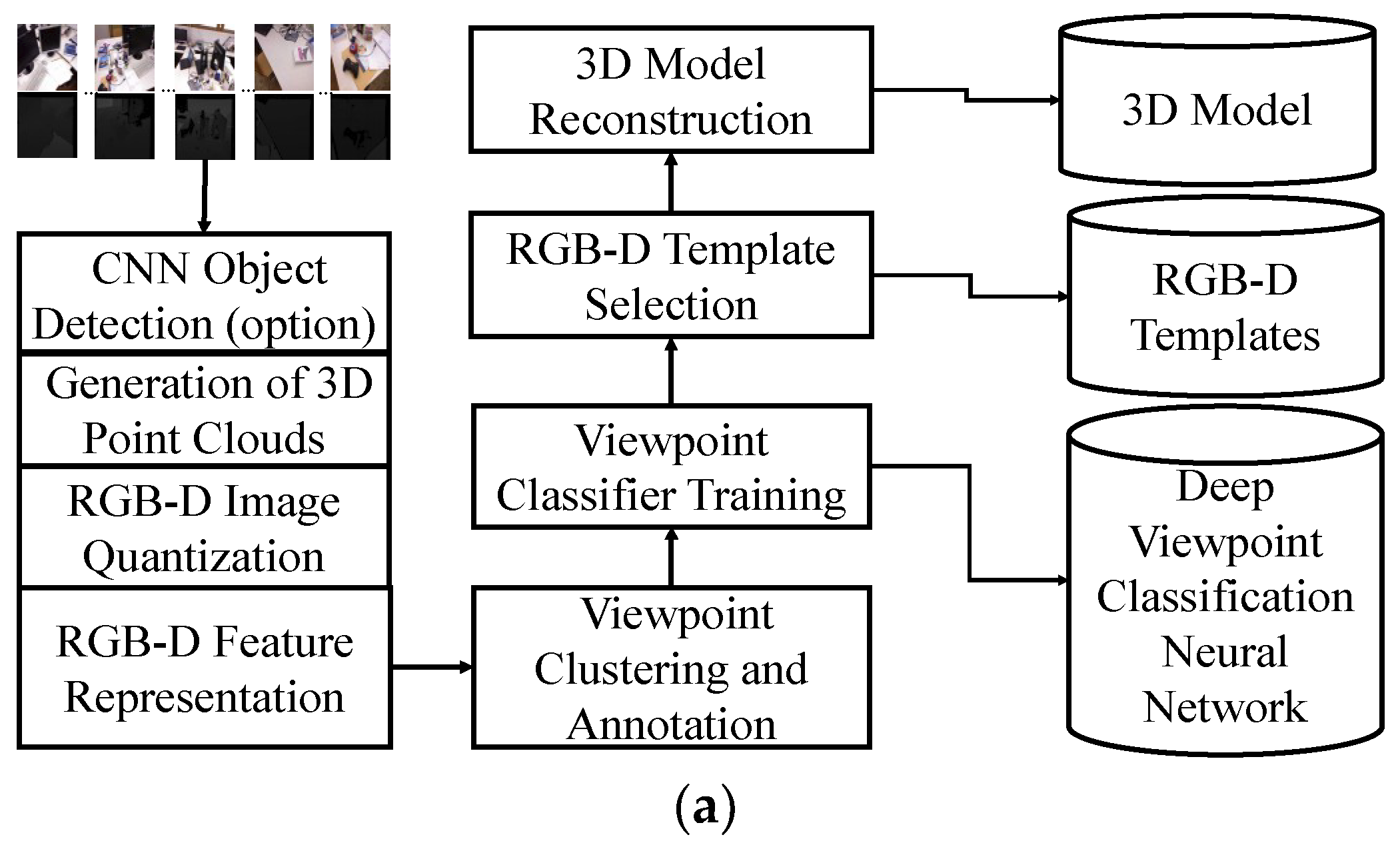
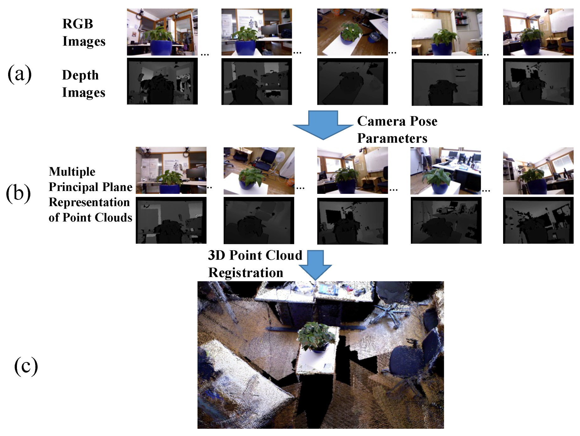
2.2.1. Template-Based 3D Scene Modeling

The core modules of the 3D scene modeling algorithm include the proposed 3D point cloud modeling using the MPPA and the training of the deep neural networks for describing the content of the scene model. In this section, we analyze these two algorithms in detail.

• 3D Point Cloud Modeling Using MPPA

In this work, we propose a deep learning approach to train a viewpoint classifier that learns the feature representation of each training RGB-D frame in a multiview video which captures the image and depth information in different views of a 3D scene. The algorithm starts by performing the 3D reconstruction algorithm, shown in Figure 2, to represent the scene as a 3D point cloud using the training depth maps and the given camera pose parameters. The 3D scene reconstruction algorithm is outlined in Algorithm 1.

Algorithm 1. Generation of 3D Scene Point Clouds.

Input: A multiview RGB-D video V characterized by n image frames, calibrated intrinsic camera parameter K and frame-by-frame external camera parameters ${\left\{{\mathrm{M}}_i\right\}}_{i=1}^n$. Output: A set of local point clouds PL and a global point cloud PG. PL is a collection of point cloud Pi which is generated from a single RGB-D image frame in the RGB-D video.PG is constructed by joining all the point cloud Pi by using the 3D point cloud registration algorithm [34]. Method: 1. for each RGB image Ii and depth image Di in V do: 1.1 Compute the i-th local point cloud Pi using Equations (2) and (4). 1.2 Perform Algorithm 2 (discussed later) to construct the binary tree of Pi and order the leave nodes as a list of super-points ${\mathsf{\Gamma }}_i={\left\{S{P}_j\right\}}_{j=1}^{\left|\right|{\mathsf{\Gamma }}_i\left|\right|}$ using the depth-first tree traversal. 1.3 for each super-point SPj in Γi do: 1.3.1 Compute the center coordinates ${\overline{\mathrm{p}}}_j$, mean color vector ${\overline{\mathrm{c}}}_j$, mean depth value ${\overline{D}}_j$, and normal vector ${\overline{\mathrm{n}}}_j$ of SPj. 1.3.2 Add the tuple (${\overline{\mathrm{p}}}_j$, ${\overline{\mathrm{c}}}_j$, ${\overline{D}}_j$, ${\overline{\mathrm{n}}}_j$) to the local point cloud Pi. 1.4 Add Pi to PL. 1.5 Join Pi into the global point cloud PG using the 3D point cloud registration algorithm [34]. Next, the major steps of the algorithm will be discussed in detail and analyzed.

The point cloud generated from Step 1.1 is first partitioned by the binary tree representation to define the set of super-points (SPs) which will be used as the basic units for the RGB-D image quantization and point cloud registration. We have two types of nodes in a binary tree: nonleave and leave nodes. A nonleave node will be decomposed into two child nodes in the binary tree. A leave node stores a small number of points that are basically located on a common 3D plane, i.e., the principal plane. We perform the depth-first-traversal process to flatten the tree as a list of leave nodes, i.e., the so-called super-points. Thus, each super-point is a leave node of the binary tree, consisting of a subset of points that describes a principal plane of the point cloud. The shape of the point cloud is finally represented as multiple principal planes (MPPs).

Let a nonleave node N contain a collection X of m points:

$$\mathrm{X}=\left[\begin{array}{l}{x}_1,y_1,z_1\\ x_2,y_2,z_2\\ \cdots \\ x_m,y_m,z_m\end{array}\right]$$

(8)

where (x_i, y_i, z_i), i = 1 to m, are the 3D points of a cloud. To perform singular value decomposition (SVD) on X, we obtain three eigenvalues λ₁, λ₂ and λ₃ (${\lambda }_1\ge {\lambda }_2\ge {\lambda }_3$) and the corresponding eigenvectors v₁, v₂ and v₃. In this work, we define the following metric to estimate the score of flatness (SF) of the local surface in N:

$$SF\left(\mathrm{N}\right)=\frac{{\lambda }_3}{{\displaystyle {\sum }_{i=1,\dots 3}{\lambda }_i}}$$

(9)

Using (9), the following rule (R1) is applied to define the type of the node N:

$$R1(\mathrm{N}):\{\begin{array}{ll}Leave,\hfill & \mathrm{if}SF\left(\mathrm{N}\right)<\gamma \hfill \\ Non-leave,\hfill & \mathrm{otherwise}\hfill \end{array}$$

(10)

where γ is a predefined threshold which controls the number of leave nodes of the resulting binary tree. Furthermore, we define the plane with the eigenvector v₃ = (v_3,x, v_3,y, v_3,z), corresponding the smallest eigenvalue of SVD(X), as the normal vector to be the principal plane (PP) of N, which can be used to compute the distance from a point p = (x, y, z) to PP:

$$d(\mathrm{p})=v_{3,x}(x-{\overline{x}}_{\mathrm{N}})+v_{3,y}(y-{\overline{y}}_{\mathrm{N}})+v_{3,z}(z-{\overline{z}}_{\mathrm{N}})$$

(11)

where $\overline{\mathrm{p}}=({\overline{x}}_{\mathrm{N}},{\overline{y}}_{\mathrm{N}},{\overline{z}}_{\mathrm{N}})={\displaystyle {\sum }_{i=1,\dots ,m}{\mathrm{p}}_i}/m$ be the center point of a node N which contains m points. Next, based on (11), rule R2 decomposing a nonleave node N into two child nodes N₁ and N₂, is defined as:

$$R2(\mathrm{N}):\{\begin{array}{ll}\mathrm{p}\in {\mathrm{N}}_1,\hfill & ifd(\mathrm{p})\ge 0\hfill \\ \mathrm{p}\in {\mathrm{N}}_2,\hfill & otherwise\hfill \end{array}$$

(12)

If N is a leave node, N is a super-point in which the v₃ is stored as the normal vector of the node. The proposed MPPA keeps a queue of nonleave nodes and removes each node in the queue one-by-one for further decomposition. Thus, the input point cloud is finally represented as a list of leave nodes (super-points) in which the shape of each super-point is modeled as its principal plane.

Let ${\mathrm{P}}_i={\{(x_j,y_j,z_j,R_j,G_j,B_j,D_j)\}}_{j=1}^{m_i}$ be the point cloud of the i-th RGB-D image frame of the training video V. Initially, we store P_i into the root note of the binary tree and set the root node to be a nonleave one. Next, based on keeping a list L_i of nonleave nodes, we build up the resulting binary tree T_i with the following summarized iterative algorithm.

Algorithm 2. Binary tree Representation of Point Cloud with the MPPA.

Input: A point cloud ${\mathrm{P}}_i={\{(x_j,y_j,z_j,R_j,G_j,B_j,D_j)\}}_{j=1}^{m_i}$. Output: A binary tree of Pi and the list of super-points ${\mathsf{\Gamma }}_i={\left\{S{P}_j\right\}}_{j=1}^{\left|\right|{\mathsf{\Gamma }}_i\left|\right|}$. Method: Initially, add Pi to the nonleave node list Li. Remove a nonleave node N from Li. Check the type of N using (10) and perform SVD to compute the principal plane of N. if N is a leave node, store the eigenvector v3 into N, which is defined as the normal vector of the principal plane in N. if N is a nonleave node do:   apply rule R2 to decompose N into two child nodes N1 and N2, which are added to Li. if Li is not empty, go to Step 2. Perform the depth-first tree traversal on the binary tree Ti to order the leave nodes as a list of super-points ${\mathsf{\Gamma }}_i={\left\{S{P}_j\right\}}_{j=1}^{\left|\right|{\mathsf{\Gamma }}_i\left|\right|}$.

As mentioned in Algorithm 1, the j-th super-point SP_j in P_i is represented as the tuple (${\overline{\mathrm{p}}}_j$, ${\overline{\mathrm{c}}}_j$, ${\overline{D}}_j$, ${\overline{\mathrm{n}}}_j$) in which ${\overline{\mathrm{n}}}_j$ is the normal vector of the principal plane that approximates the shape of the points in SP_j. For each point in SP_j, we set the color and depth values of the corresponding pixel in 2D image to be ${\overline{\mathrm{c}}}_j$ and ${\overline{D}}_j$, respectively. This process generates the super-pixels of the input RGB and depth images. Figure 3 shows an example of representing an RGB-D image as a point cloud, which is processed to generate the super-point-based point cloud and super-pixel-based RGB-D images using the proposed MPPA.

• 3D Scene Modeling Using Deep Learning

Recently, deep learning has been recognized to be a successful approach in the research of artificial intelligence [43,45,46]. The key to the success of deep learning is the labeling of a large amount of training data because the number of parameters to be trained in a deep learning neural network is often very huge. However, the training data labeling cost is often so high and limits the applications of deep learning in research areas wherein it is impossible to prepare a large amount of training data by human annotation. To deal with the difficulty, for 3D scene modeling, we propose an unsupervised deep learning neural networks which use the automatically labeled training data with the proposed 3D point cloud processing algorithms. The proposed learning approach can be categorized as the methodology of self-taught learning, which is recognized to be an effective method for training a supervised-learning based neural network without using a tedious human annotated dataset.

In this work, the convolutional-based deep viewpoint classification neural network (DVCNN) is trained in the 3D scene modeling phase. As shown in Figure 4, the auto-encoder neural networks, which are variants of the semantic segmentation neural network (SegNet) [47], can be used for RGB-D deep feature prelearning. The layers of the encoder and decoder network in Figure 4 are topologically identical to the layers of auto-encoder and decoder in SegNet except that we use ADAM as the optimizer instead of SGD since the ADAM achieves better training performance. In this work, we also discard the last softmax layer of the decoder and use a 1 × 1 convolution layer with ReLU instead.

Given a training RGB-D video V of n image frames for 3D scene modeling, for each RGB image I and depth image D in V, the proposed Algorithm 1 generates the corresponding quantized RGB image qI and quantized depth image qD, and then produces the training data sets: RGB-dataset and depth-dataset which consist of collections of RGB image tuples ${(I_j,q{I}_j)}_{j=1}^n$ and depth image tuples ${(D_j,q{D}_j)}_{j=1}^n$, respectively. Using a generic back-propagation gradient descent optimization algorithm, the RGB-dataset (depth-dataset) can be applied to train the RGB-deep feature learning neural network (depth-deep feature learning neural network) using the loss function defined as follows:

$$loss=\frac{1}{n}{\displaystyle \sum _{j=1}^n\left|\right|q{I}_j-{\widehat{I}}_j|{|}_2}$$

(13)

where ${\widehat{I}}_j$ is the image generated by the feature learning neural network if the j-th input image I_j is applied for training. As shown in Figure 4c, a deep feature learning neural network (DFLNN) can also be used to recover the depth information from the input RGB image by applying the training dataset which consists of a collection of image tuples ${(I_j,D_j)}_{j=1}^n$ to train the resulting depth recovering neural network (DRNN). The last layer of both DFLNN and DRNN is a 1 × 1 convolutional layer, which reduces the dimensionality of the output of the RGB-decoder (or depth-decoder), i.e., the prelearned deep features, to the shape of the original input.

The performance of the above neural networks for deep feature pretraining is obviously limited by the size of training datasets. This is the so-called overfitting problem of deep neural networks. Instead of using the auto-encoders to compute the deep features of the training RGB-D images, in our approach, we directly cascade the visual features of all super-pixels into a feature vector to characterize the content of an input RGB image. Next, we perform the well-known k-means clustering on the collection of these visual feature vectors to group the training RGB-D images into clusters. With each cluster representing a viewpoint, the clustering results automatically generate the viewpoint (vp) labels of the training RGB-D images. This forms a collection of viewpoint training tuples ${(I_j,v{p}_j)}_{j=1}^n$ for training the proposed viewpoint classifier which is a variant of the VGG convolutional neural network (CNN) [43]. As shown in Figure 5, the trained deep viewpoint classification neural network (DVCNN) is accurate in annotating the viewpoint of an input RGB image because it is transferred from the effective VGG neural network. Note that the input to the DVCNN is only a single RGB image. That is because only a single RGB image is used for 3D model updating and inspecting in the model updating phase.

The final step to build up the 3D scene model is the selection of templates that play an important role in the estimation of camera external parameters for the input RGB image captured by a moving RGB camera in a drone. Let VP_i be the set of training RGB-D images that are labeled as the viewpoint i by the DVCNN. The training RGB-D image Φ_i is defined to be the template of viewpoint i if

$${\mathsf{\Phi }}_i=\arg \underset{I_j\in V{P}_i}{\max }\mathrm{Pr}(I_j)$$

(14)

where Pr(I_j) is the probability of the input RGB image I_j labeled as viewpoint i using the DVCNN. The pose parameters of these templates are also stored in the 3D scene model for the purpose of estimating the pose parameters of the input RGB image in the model updating phase.

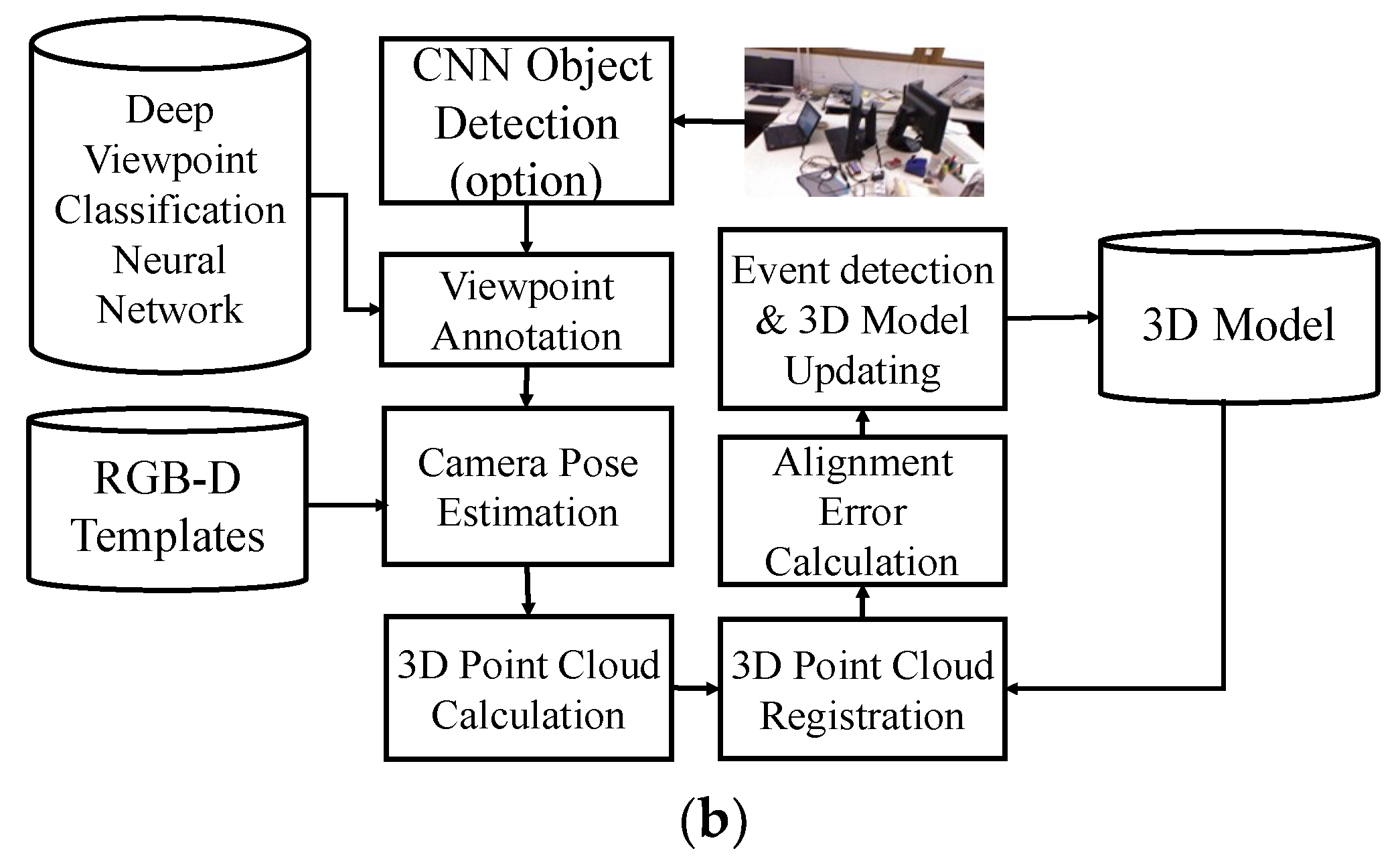
2.2.2. The Pose Estimation Algorithm

The usage of a highly mobile drone facilitates the modeling task of a 3D outdoor scene. The selected templates to model the target 3D scene also play an important role in the application of visual inspection because the associated GPS information of templates is useful to define the checkpoints of the scene. In the inspection phase, we navigate the drone to the GPS locations of the templates and capture individual RGB images which can be used to detect abnormal events that occur in the real-world scene. Furthermore, the scene under surveillance is often changing slightly along the timeline. It is quite important to keep the model up-to-date when we load the model into a 3D scene surveillance application. Basically, the 3D model records the background information which corresponds to the normal situation of the scene under surveillance. On the contrary, an abnormal event can be detected in a specific checkpoint if the matching error between the current input RGB image and the corresponding RGB template is large. However, the detection accuracy is often limited by this simple scheme since the captured RGB image in a checkpoint is often not the same as the corresponding template RGB image as the location of the navigated drone contains an error using the prestored GPS information of templates. This leads to the requirement of the pose estimation algorithm that recovers the depth image and external camera parameters using an alignment algorithm between the input RGB image and the corresponding template RGB image.

In the model updating phase, given an RGB image I captured from an unknown location of the scene, the proposed pose estimation algorithm is an iterative procedure consisting of four major steps: (1) search for a suitable template that samples the possible appearance of the model in the input image I using the proposed DVCNN; (2) compute the point cloud of I for generating the super-points and the super-pixels; (3) compute the transformation matrix that aligns the input image I with the template in terms of the visual features of super-pixels; (4) fine tune the pose parameters and depth map of I by an iterative closest point (ICP) algorithm [48,49]. Given an input RGB image, the pose estimation algorithm uses the external camera parameters and depth map of the corresponding template as the initial coarse parameters to compute the first 3D point cloud. Incorrect pose parameters would generate a larger error when we register the current point cloud with the model point cloud in a 3D space. The iterative pose estimation stops when the registration error is minimized.

With object inspection as an example, Figure 6 shows the proposed scheme to estimate the external camera parameters of the input images, which are often unknown when we use a moving camera to conduct 3D object inspection. To deal with this issue, the proposed image-based scene (object) modeling can be used to accurately estimate the depth map as well as the external camera parameters of the input image. The first step of the proposed drone-based surveillance scheme is to detect the target objects in the input RGB I_j using the well-proved CNN object recognition system [43]. Next, with the detected object O as the input data, the proposed MPAA returns a set of discriminative visual features. Let i be the viewpoint class of the input image I_j which is annotated by the proposed DVCNN. This implies that the i-th RGB-D template Φ_i would be retrieved from the image-based 3D model. Initially, the depth map of the i-th template Φ_i is set to be the depth image D_j of I_j. We also set the external camera parameters of Φ_i as the initial parameters for the test image I_j. Obviously, the external camera parameters should be modified because it is not possible for the positions of the cameras to capture the test image and the template to be the same.

In this work, we use the well-known RANSAC feature corresponding algorithm [50] to align the set of discriminative visual features of Φ_I, i.e., the features of the super-pixels, with those of I_j. Let the output of the RANSAC algorithm be the corresponding collection of r tuples:

$${\mathsf{\Omega }}_{O_j}^{{\mathsf{\Phi }}_i}={\left({\mathrm{x}}_a^{O_j},{\mathrm{x}}_a^{{\mathsf{\Phi }}_i}\right)}_{a=1}^r$$

(15)

where ${\mathrm{x}}_a^{O_j}$ (${\mathrm{x}}_a^{{\mathsf{\Phi }}_i}$) is a pixel in O_j (Φ_i). Note that the intrinsic camera parameters of the moving camera should be calibrated in advance in both the modeling and inspection phases. To initially estimate the external camera parameters of O_j with those of the template Φ_i, for each pixel in O_j (Φ_i), the point set ${\mathrm{p}}_{O_j}^{}={({\mathrm{p}}_a^{})}_{a=1}^r$ (${{\mathrm{p}}^{\prime }}_{{\mathsf{\Phi }}_i}^{}={({\mathrm{p}}_a^{\prime })}_{a=1}^r$) in the world coordinate system is computed using (2) and (4). Next, to register points in ${\mathrm{p}}_{O_j}^{}$ with those in ${{\mathrm{p}}^{\prime }}_{{\mathsf{\Phi }}_i}^{}$, the ICP algorithm produces the transformation matrix ${\mathrm{M}}_j^i=[{\mathrm{R}}_j^i|{\mathrm{t}}_j^i]$ in the world coordinate system, where ${\mathrm{R}}_j^i$ and ${\mathrm{t}}_j^i$ are the rotation matrix and the translation vector, respectively. ${\mathrm{M}}_j^i=[{\mathrm{R}}_j^i|{\mathrm{t}}_j^i]$ is actually the external camera parameters that transform the point cloud ${\mathrm{p}}_{O_j}^{}$ to point cloud ${{\mathrm{p}}^{\prime }}_{{\mathsf{\Phi }}_i}^{}$ in the world coordinate system. Thus, the fine-tuned external camera parameters of O_j for building up the real 3D point cloud using the depth map of O_j are:

$${\mathrm{M}}_{4\times 4}^{O_j}={\mathrm{M}}_j^i{\mathrm{M}}_{4\times 4}^{{\mathsf{\Phi }}_i}=\left[\begin{array}{cc}{\mathrm{R}}_{j,3\times 3}^i& {\mathrm{t}}_{j,3}^i\\ 0& 1\end{array}\right]\left[\begin{array}{cc}{\mathrm{R}}_{3\times 3}^{{\mathsf{\Phi }}_i}& {\mathrm{t}}_3^{{\mathsf{\Phi }}_i}\\ 0& 1\end{array}\right]$$

(16)

where ${\mathrm{M}}_{4\times 4}^{{\mathsf{\Phi }}_i}$ are the external camera parameters of the template Φ_i. The underlying concept of the proposed pose estimation algorithm is based on the assumption that a pair of correspondence pixels of the same visual features in two images would be unprojected to the same point in 3D space. Moreover, errors exist in the coarse estimated depth image and external camera parameters which are eliminated by the transformation matrix ${\mathrm{M}}_j^i$ using the ICP algorithm.

The modified point cloud of the input image is then analyzed to generate the super-pixels of the RGB and depth images. Inputting these new versions of super-pixel features into the pose estimation algorithm, the registration error between the current point cloud and the model point cloud is minimized. To complete the discussion of the pose estimation, we design a method to compute the error by registering the point cloud P of the target model with the current point cloud P_j of the input image I_j. Once again, the RANSAC algorithm is used to establish the 3D super-point correspondence set in terms of the feature vectors of super-points, which are defined in (6). Next, based on the super-point correspondence set, the transformation ${\mathrm{M}}_j^{}=[{\mathrm{R}}_{j,3\times 3}^{}|{\mathrm{t}}_{j,3}^{}]$ between P and P_j is computed. For each super-point p in P_j, we compute the super-point ${\mathrm{p}}^{\prime }$ in the model, which contains the point ${\mathrm{M}}_j\mathrm{p}$. Using their features, then the error between P and P_j is defined as

$$E=\frac{1}{n}{\displaystyle \sum _{i=1}^n\left|\right|{\overrightarrow{f}}_i}-{{\overrightarrow{f}}^{\prime }}_i|{|}_2$$

(17)

where n is the number of super-points in P_j; ${\overrightarrow{f}}_a$ is the feature vector of the i-th super-point p_i in P_j; ${{\overrightarrow{f}}^{\prime }}_i$ is the feature vector of the corresponding super-point ${\mathrm{p}}_i^{\prime }$ in the model. The proposed model-based pose estimation algorithm is summarized as shown in Algorithm 3.

Algorithm 3. Model-based Pose Estimation

Input: A single RGB image I Output: The pose parameters of I and the registration error E Method: Input I to the DVCNN to obtain the viewpoint class v and retrieve the template Φv from the prestored database. Set the pose parameters of I to be depth image and external camera parameters of Φv. Compute the 3D point clouds ${\mathrm{p}}_I^{}={({\mathrm{p}}_a^{})}_{a=1}^r$ and ${{\mathrm{p}}^{\prime }}_{{\mathsf{\Phi }}_v}^{}={({\mathrm{p}}_a^{\prime })}_{a=1}^r$ for I and Φv, respectively using (2) and (4). Perform the MPAA to compute the super-points and super-pixels of I and Φv. Perform the RANSAC algorithm to generate the pixel correspondences ${\mathsf{\Omega }}_I^{{\mathsf{\Phi }}_v}={\left({\mathrm{x}}_a^I,{\mathrm{x}}_a^{{\mathsf{\Phi }}_v}\right)}_{a=1}^r$ between I and the RGB image in Φv in terms of their visual features of key points (super-pixels). Perform the ICP algorithm to register PI and ${{\mathrm{p}}^{\prime }}_{{\mathsf{\Phi }}_v}^{}$, and compute the transformation matrix ${\mathrm{M}}_I^v=[{\mathrm{R}}_{I,3\times 3}^v|{\mathrm{t}}_{I,3}^v]$. Fine tune the external camera parameters of I to be ${\mathrm{M}}_{4\times 4}^{}$ using (16). Compute the final point cloud PI of I and perform the RANSAC algorithm is used to establish the 3D super-point correspondence set between PI and the model point cloud Pm in terms of the feature vectors of super-points, which are defined in (6). Perform the ICP algorithm to register PI and Pm, and compute the transformation matrix ${\mathrm{M}}_I^m=[{\mathrm{R}}_{I,3\times 3}^m|{\mathrm{t}}_{I,3}^m]$. Compute the inspection error E using (17). ifE is not changed again, return the pose parameters of I and E; else goto 4.

3. Results

The system is implemented on a PC with Intel Core i7 3.4 GHz CPU and NVIDIA GeForce 9800 GT. The RGB-D benchmark provided by the Technical University of Munich [44] is used to verify the effectiveness of our approach in terms of the accuracy of the viewpoint classification and pose estimation. In this benchmark, several datasets [51] including aligned color and depth sequences captured with a single RGB-D moving camera are provided. The accurate ground-truth of each frame’s camera pose is also provided, which is measured by an external motion capture system. The image frames of each dataset are separated into two disjoint sets: a training dataset and a test dataset. Figure 7 shows an example of an RGB frame in each dataset.

In the application of object modeling and inspection, the CNN object detector is applied to locate the target objects in the RGB images. To train the CNN object detector, the set of bounding boxes that locate the target objects in the training RGB image frames is obtained by human annotation. The accuracy of the resulting CNN object detection obviously affects the accuracy of the modeled 3D object. To verify the effectiveness of the usage of CNN object detector in our application, both the model-specific and global CNN object detectors are trained using a single dataset and all datasets, respectively. Figure 8 shows the performance comparison between these two modes of CNN object detectors. One of the advantages of the usage of the global CNN object detector is that we just need to train a single CNN object detector which detects all objects in different models. However, the performance of the global CNN object detector is not good enough to provide accurate object modeling results. On the contrary, the model-specific object detector achieves average accuracy of up to 98.62% and thus guarantees the accuracy of the resulting 3D object model. Thus, we train multiple model-specific CNN object detectors which are further integrated to achieve the goal of detecting all objects under surveillance. The model-specific CNN object detector that gives the largest probability on the detected object is used to annotate the object in a test RGB image. This preserves the high accuracy advantage of the model-specific CNN object detector, which can be verified by the results shown in

Table 1. The confusion matrix of integrating multiple model-specific CNN object detectors for detecting all objects under surveillance.

	Classification Results	Freiburg1_Plant	Freiburg1_Teddy	Freiburg2_Coke	Freiburg2_Flower	Freiburg3_Cabinet	Freiburg3_Teddy
Input Classes
freiburg1_plant		97	3	0	0	0	0
freiburg1_teddy		1	97	0	2	0	0
freiburg2_coke		0	0	98	2	0	0
freiburg2_flower		0	0	3	97	0	0
Freiburg3_cabinet		4	0	0	0	94	2
freiburg3_teddy		1	0	0	0	2	95

.

The second experiments demonstrate the effectiveness of the proposed viewpoint classification. Figure 9 shows the view classification results using the dataset ‘freiburg3_teddy’. The RGB template of a viewpoint and those of test images that are classified to the viewpoint class are very similar in terms of subjective evaluation. Given the training dataset ‘freiburg3_teddy’, with the clustering results as the viewpoint labels, the recognition accuracy of our viewpoint classifier achieves 98.24% without suffering from the overfitting problem.

To compare the performance of our approach with other state-of-the-art methods in pose estimation [39,40,52,53], five typical datasets are selected as test samples. In [39,52], the compared approaches are model-based methods which are similar to our approach. In [40,53], the authors proposed RGB-D SLAM systems. Some postprocessing methods, such as global optimization are used to modify the global camera trajectory in these methods.

Table 2. Camera pose error for datasets with ground-truth from [44] in terms of RMSE of the relative error. The value of k is the number of training RGB images in a viewpoint class in our approach, and the stride to select the key-frames from the training datasets in other approaches.

Sequence	RMSE of the Relative Camera Pose Error
	Our Approach				Multiresolution Map [52]	RGB-D SLAM [40]
	k = 1	k = 5	k = 10	k = 20
freiburg1 desk2	1.50 × 10−16	0.024	0.052	0.108	0.060	0.102
freiburg1 desk	1.39 × 10−16	0.019	0.041	0.086	0.044	0.049
freiburg1 plant	1.22 × 10−16	0.015	0.033	0.066	0.036	0.142
freiburg1 teddy	1.62 × 10−16	0.020	0.044	0.087	0.061	0.138
freiburg2 desk	2.84 × 10−16	0.005	0.010	0.018	0.091	0.143

summarizes the experimental results. The first column is the dataset name. The remaining columns are the results for the root mean square error (RMSE) of the relative errors. The relative error is the translational drift in m/s between the estimated pose and the ground-truth. The parameter k is the number of RGB training images in a viewpoint class for training the viewpoint classifier. For each viewpoint class, we select a template; a larger value of k implies that fewer templates are selected in the training sequences to build up the 3D model for inspecting the target scene or object in the testing phase. Since a large amount of redundancy could exist in two consecutive frames of each sequence (dataset), we can actually use very few frames to reconstruct a 3D model. The usage of fewer templates also highly reduces the time complexity to estimate the pose of each frame in order to achieve the goal of 3D object reconstruction in real-time. As shown in Figure 10, compared with other state-of-the-art approaches, the proposed method is not sensitive to the value of k. Accordingly, the proposed method can use very few templates to model a 3D scene without sacrificing the accuracy of pose estimation. Figure 11a shows an example of the 2D trajectory error of the proposed method using the test sequence ‘freiburg1_desk’; the reconstructed 3D scene using the selected templates is also shown in Figure 11b. Figure 11(a1,a2) are the 2D trajectory error without and with the removement of the outliers of corresponding pairs, respectively, when using Algorithm 3 to estimate the poses. In these two examples, the trajectory of the 3D poses is projection to the xy plane. The black trajectory is the ground truth. The blue trajectory is the estimated poses. The red lines are the error between the ground truth and the estimated poses. From Figure 11(a3), the errors are reduced after removing the outliers of the corresponding pairs. With the usage of the GPU, our system can process more than 30 frames per second. This ensure to apply our algorithms to construct real-time video-based applications.

4. Discussion

According to the experimental results, we can outline several interesting research findings for 3D computer vision:

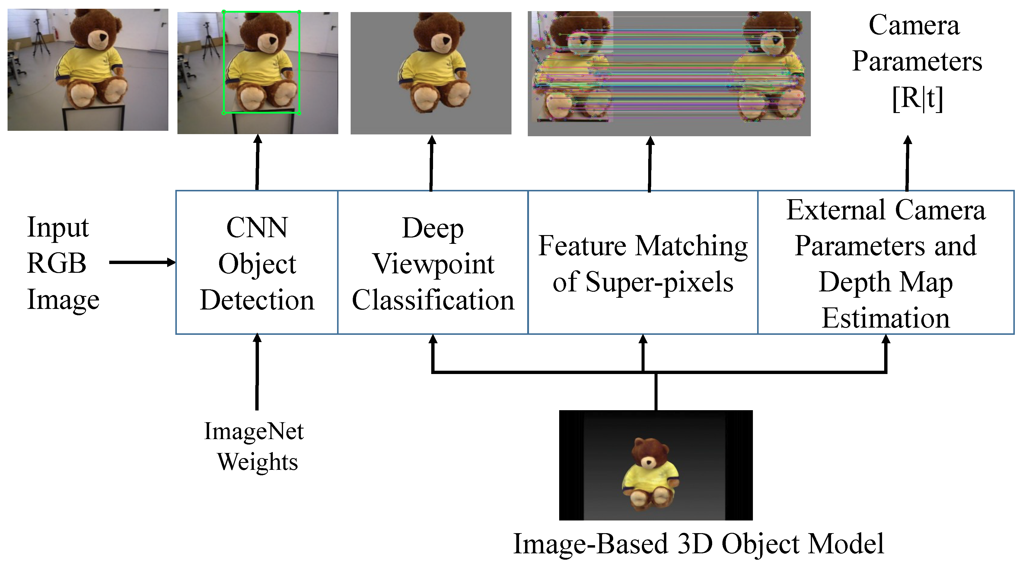
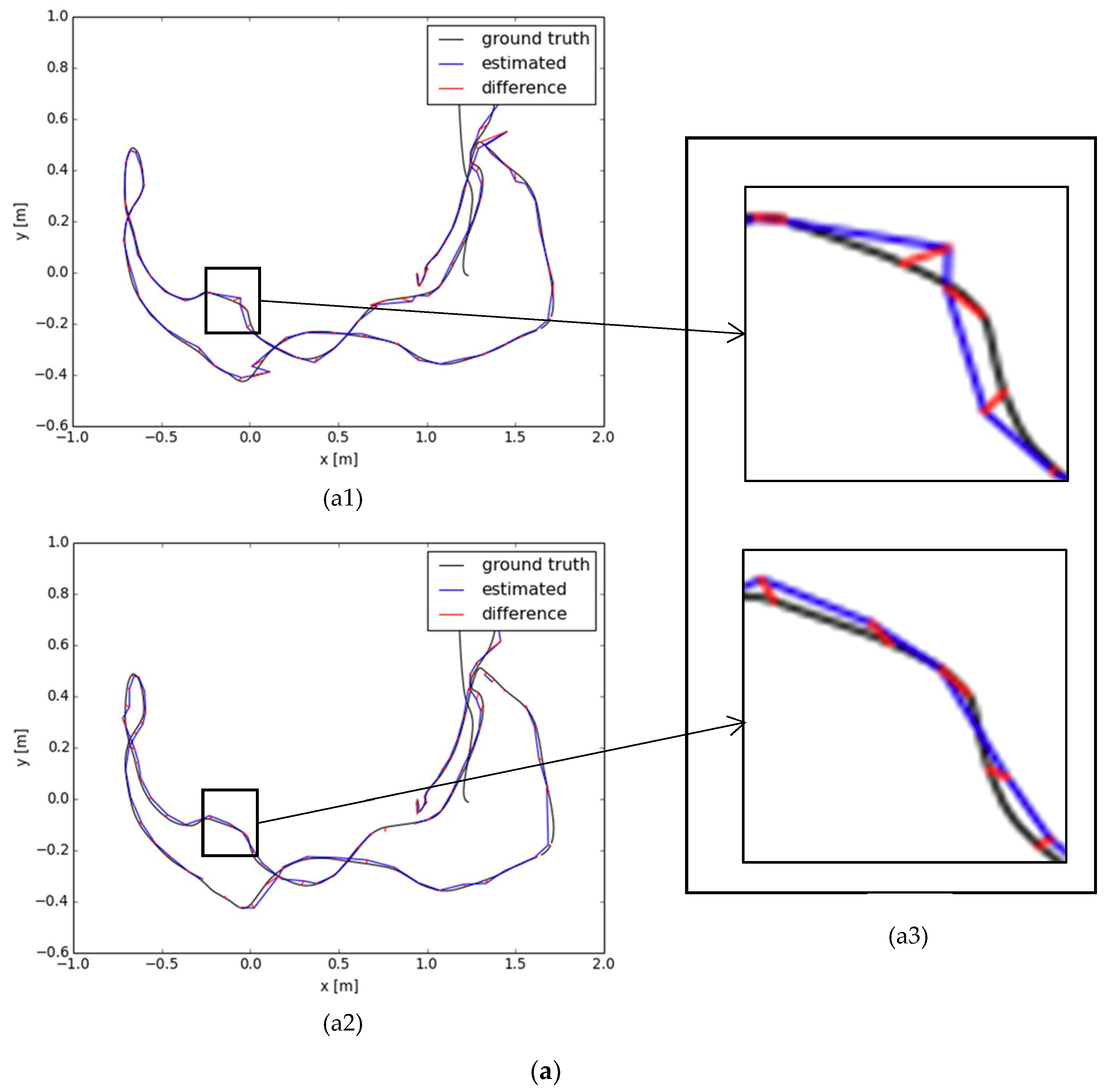
• To the best of our best knowledge, there are very few researchers working on the problem of pose estimation using a single RGB image. Conventional pose estimation algorithms use a sequence of RGB images to compute the depth map and the external camera parameters. However, this highly increases the complexity of the resulting pose estimation. On the contrary, in this work, the input to the model-based pose estimation algorithm is only a single image. This facilitates the real-time reconstruction of 3D models.
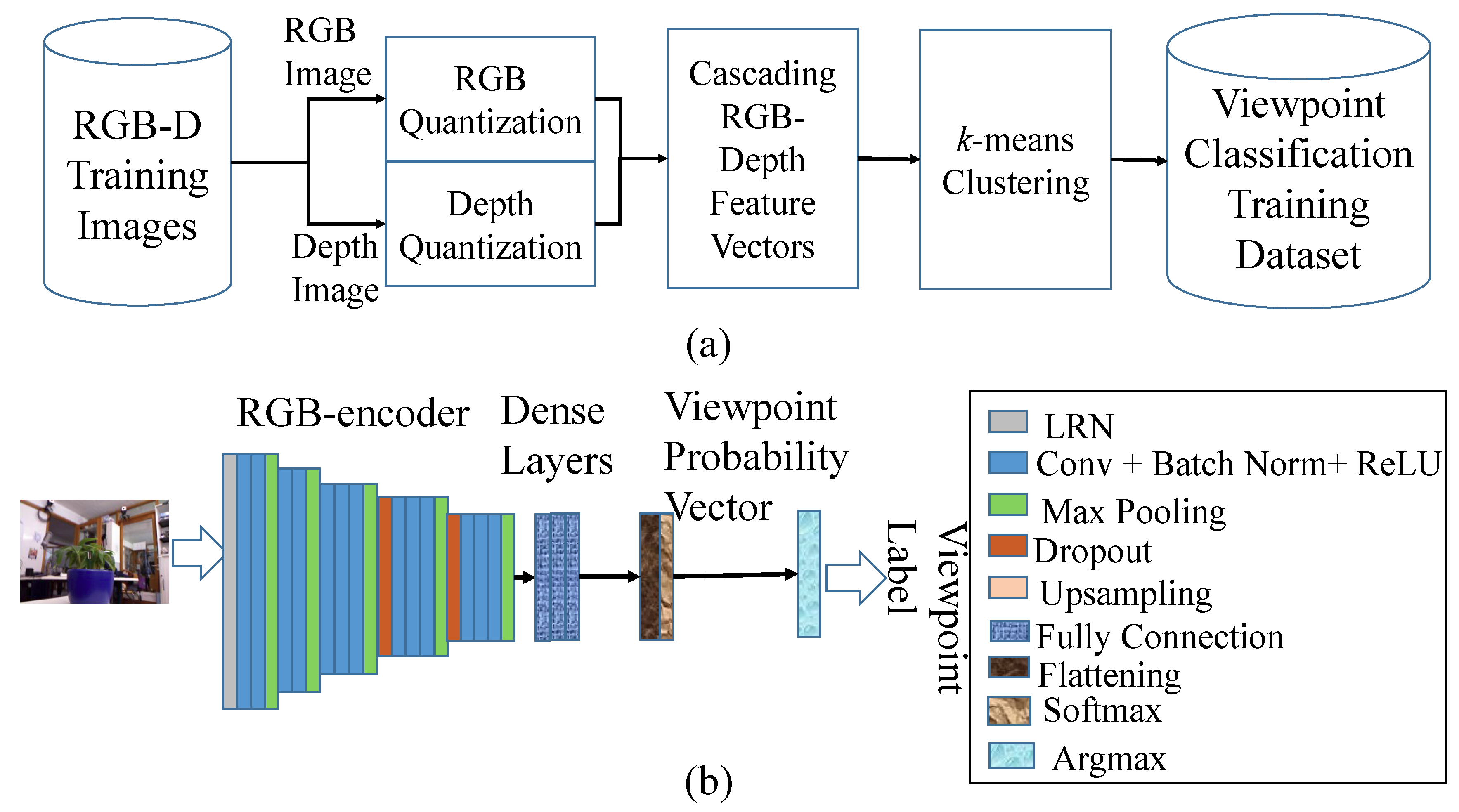
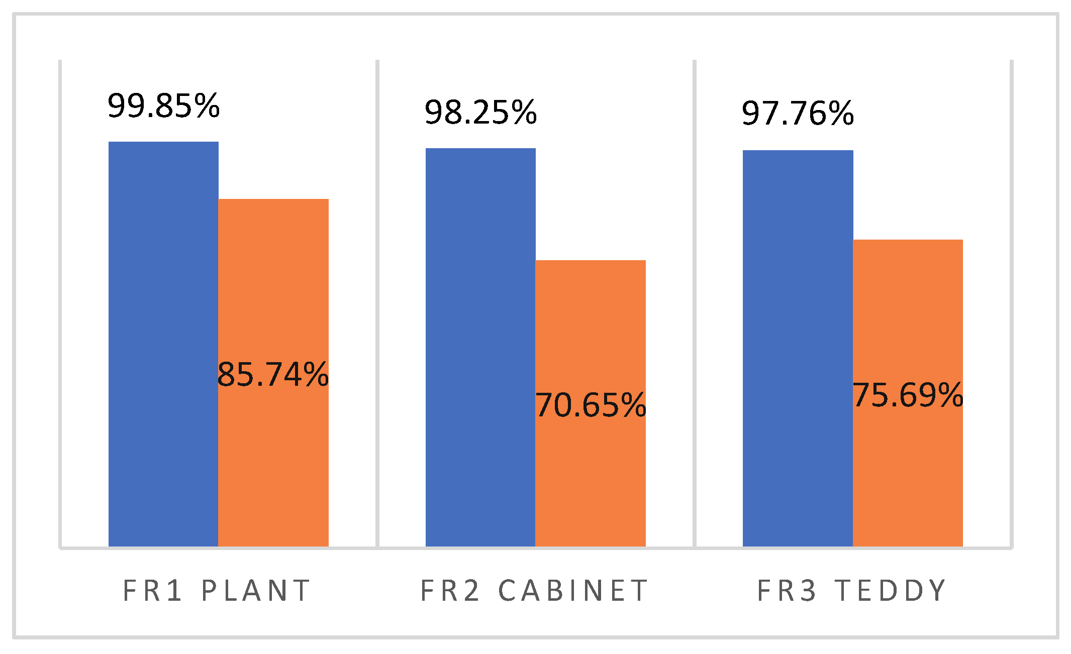
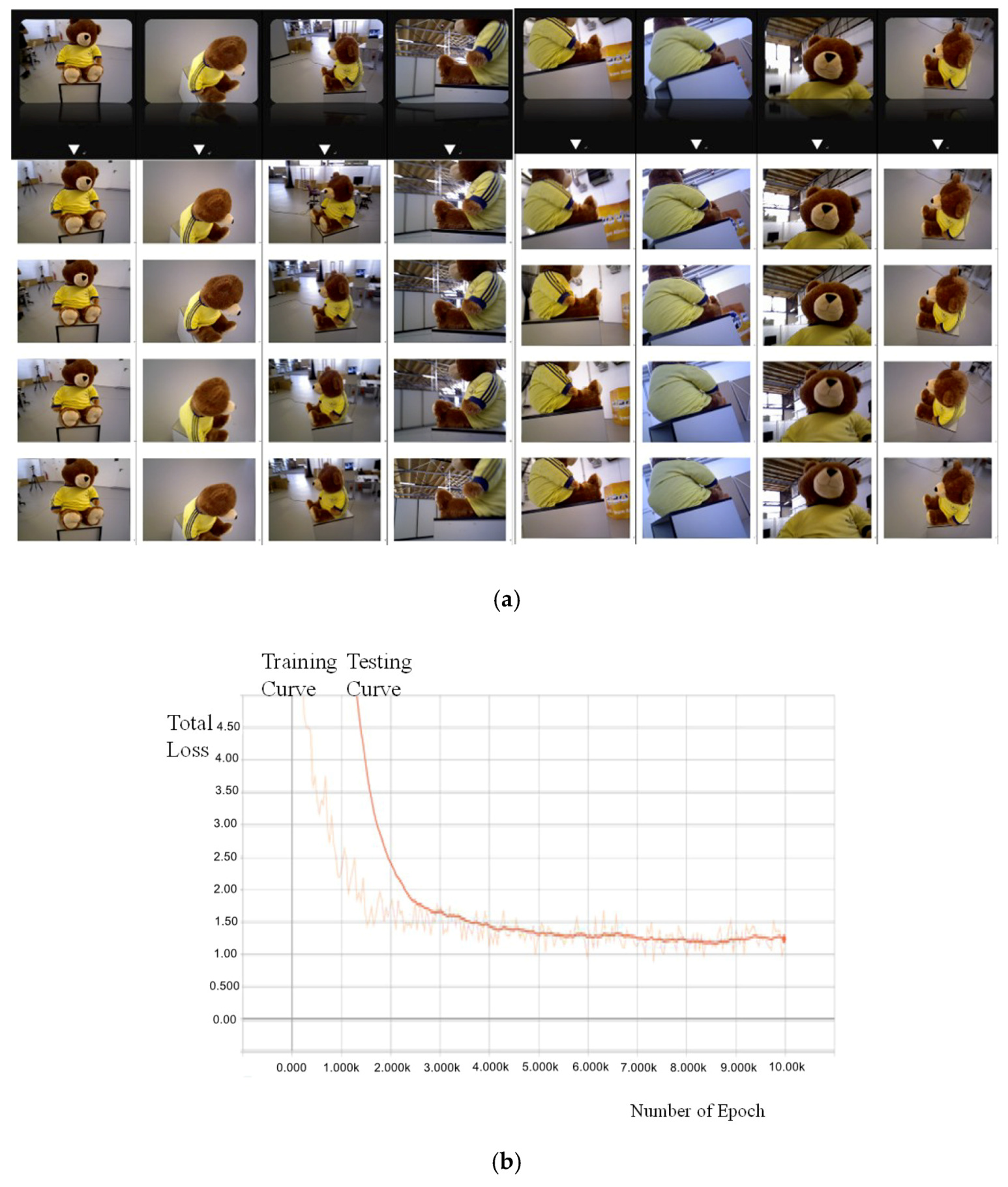
• The tedious human annotation effort required to prepare a large amount of training data for improving the recognition accuracy of the DVCNN is avoided by representing scene point clouds as a collection of super-points using the MPPA algorithm. Although the number of training RGB-D image frames for 3D scene modeling is often small, the average recognition rate for viewpoint classification using the DVCNN achieves 98.34% according to our experimental results. Moreover, the learning curves of testing and learning for the DVCNN closely coincide with each other. This implies the overfitting problem of conventional deep neural networks is solved even when the training data is automatically labeled.
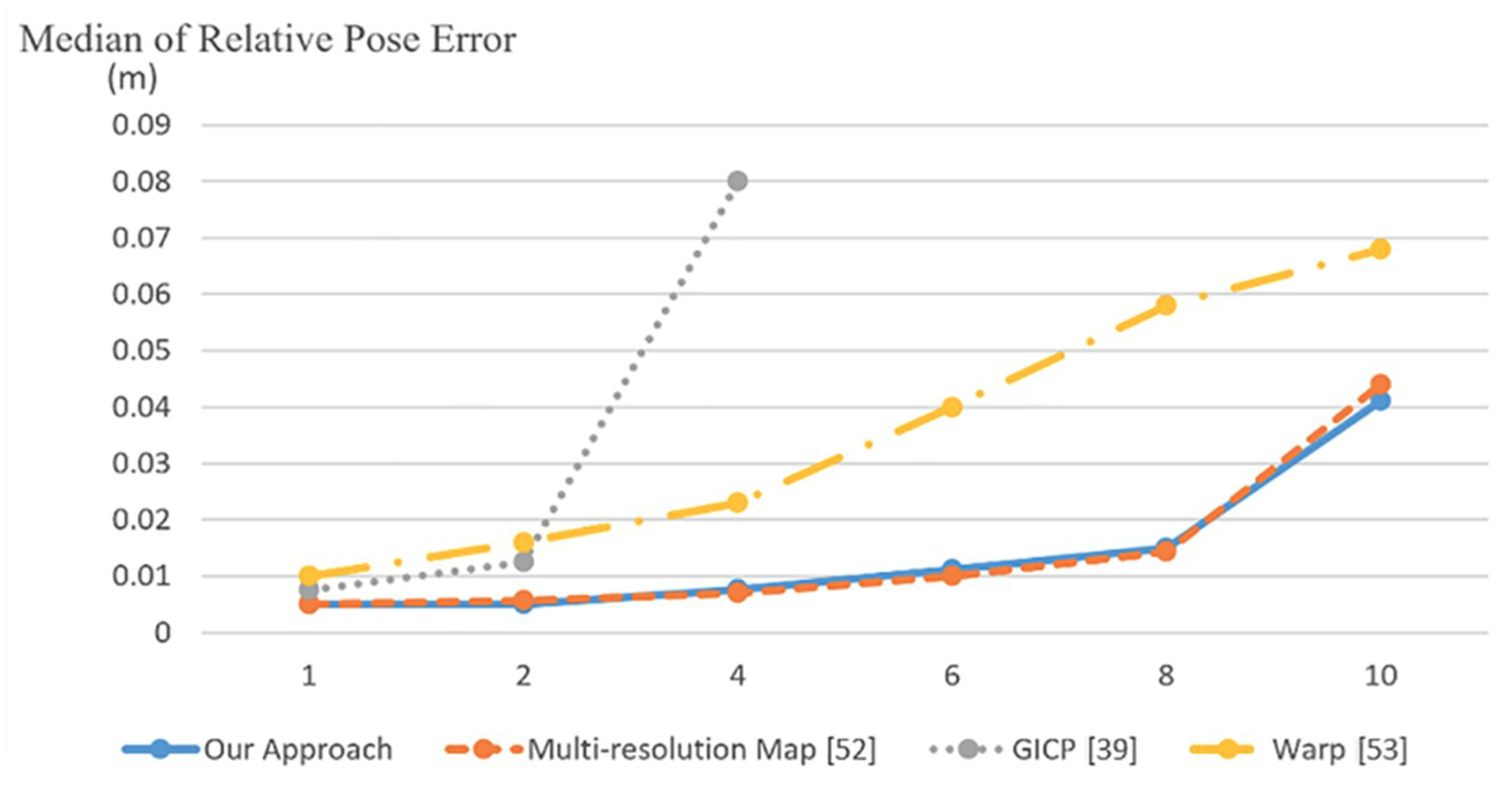
• The performance of the proposed pose estimation is obviously dependent on the number of templates used to model a 3D scene. As shown in Table 2, the usage of fewer templates for 3D scene modeling leads to more significant errors in registration between the current point cloud, generated by the input RGB image, and the model point cloud. In the application of abnormal event detection, the registration error introduced by the model-based pose estimation algorithm should be minimized to a very small degree in order to reduce the number of false positives in the construction of an event alarm system. Thus, we suggest using more templates in 3D model reconstruction even though it increases the computational complexity.
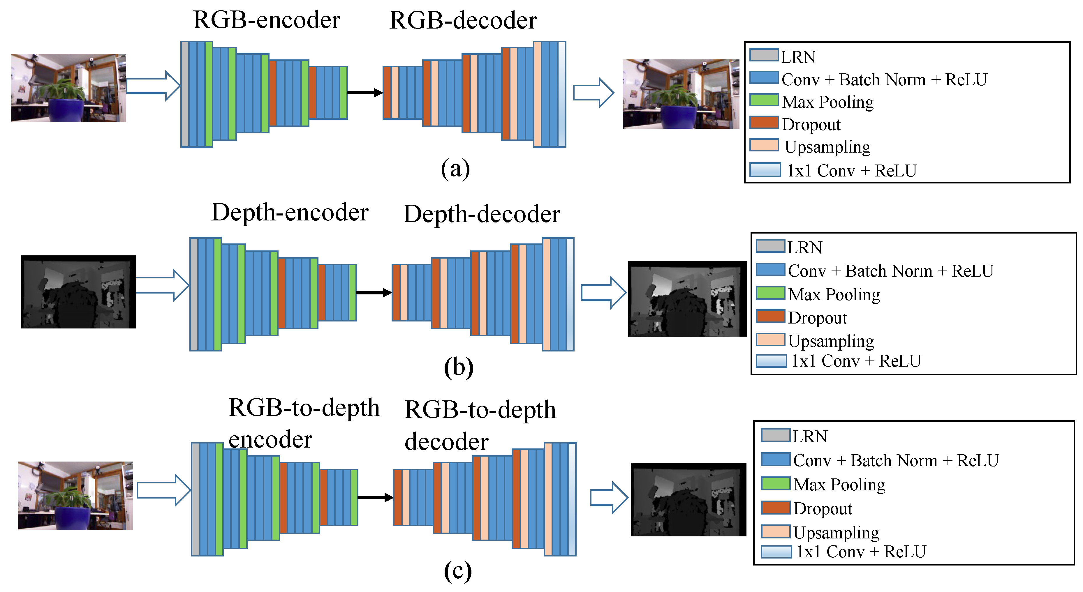
• The usage of deep features obtained by the deep neural networks shown in Figure 4 is not suggested when the training datasets are not large enough. The usage of features of super-points and super-pixels offers good discrimination power in the learning of the DVCNN according to our experimental results. The proposed MPAA is actually much like the conventional PCA dimensionality reduction technique. This implies that the claim that deep learning outperforms traditional learning schemes in all aspects of applications is a pitfall.

The proposed 3D scene modeling can model the background information fast and accurately. Thus, a real-time vision-based scene surveillance system can be easily constructed using a simple background subtraction algorithm. Moreover, the problem of unstable background degrading the performance of the simple background subtraction scheme for visual inspection is avoided since our pose estimation algorithm eliminates the slight changes in the model under surveillance along the timeline using the model updating scheme.

5. Conclusions

In this paper, we have presented a model-based scalable 3D scene modeling system. The contributions of the proposed method include: (1) starting from the computation of the point cloud of an input RGB-D image, the MPPA automatically labels training image frames to prepare training datasets for training deep viewpoint classification; (2) the fusion of multiple model-specific CNNs can detect multiple objects under surveillance accurately; (3) the viewpoint classifier searches the best template images for constructing a high quality image-based 3D model; (4) in the model updating phase, the usage of the template-based 3D models speeds up the process of pose estimation by using a single RGB image. In our experiments on publicly available datasets, we show that our approach gives the lowest overall trajectory error and outperforms the state-of-the-art methods.

The proposed approach could be easily applied for geodesy and remote sensing. For example, a high-quality 3D model of an area with frequent earth-rock flow could be built by traditional methods [1,2]. After a hurricane, the damage of this area could be detected by pictures captured by a low-cost unmanned drone. For AR or face recognition applications, the 3D scene model or face model could be constructed from video captured by a low-cost RGB-D camera. The constructed 3D model could also be used for 3D printing.

In the next step of our research, we plan to explore a large-scale AR interaction system based on this template-based 3D scene or object modeling. Furthermore, based on the reconstruction models, we want to extend our approach to 3D object recognition, detection, segmentation, reconstruction, and printing.

References

1. Wolf, P.R.; Dewitt, B.A. Elements of Photogrammetry: With Applications in GIS; McGraw-Hill: New York, NY, USA, 2000. [Google Scholar]
2. Ackermann, F. Airborne laser scanning–present status and further expectations. ISPRS J. Photogramm. Remote Sens. 1999, 54, 64–67. [Google Scholar] [CrossRef]
3. Davison, A.; Reid, I.; Molton, N.; Stasse, O. MonoSLAM: Real-time single camera SLAM. IEEE Trans. Pattern Anal. Mach. Intell. 2007, 29, 1052–1067. [Google Scholar] [CrossRef] [PubMed]
4. Seitz, S.M.; Curless, B.; Diebel, J.; Scharstein, D.; Szeliski, R. A comparison and evaluation of multi-view stereo reconstruction algorithms. In Proceedings of the 2006 IEEE Computer Society Conference on Computer Vision and Pattern Recognition, New York, NY, USA, 17–22 June 2006; Volume 1, pp. 519–528. [Google Scholar]
5. Furukawa, Y.; Curless, B.; Seitz, S.M.; Szeliski, R. Towards internet-scale multi-view stereo. In Proceedings of the 2010 IEEE Computer Society Conference on Computer Vision and Pattern Recognition, San Francisco, CA, USA, 13–18 June 2010; pp. 1434–1441. [Google Scholar]
6. Furukawa, Y.; Ponce, J. Accurate, dense, and robust multi-view stereopsis. IEEE Trans. Pattern Anal. Mach. Intell. 2010, 32, 1362–1376. [Google Scholar] [CrossRef] [PubMed]
7. Snavely, N.; Seitz, S.M.; Szeliski, R. Modeling the world from internet photo collections. Int. J. Comput. Vis. 2008, 80, 189–210. [Google Scholar] [CrossRef]
8. Guan, W.; You, S.; Neumann, U. Recognition-driven 3D navigation in large-scale virtual environments. In Proceedings of the IEEE Virtual Reality, Singapore, 19–23 March 2011. [Google Scholar]
9. Alexiadis, D.S.; Zarpalas, D.; Daras, P. Real-time, full 3-D reconstruction of moving foreground objects from multiple consumer depth cameras. IEEE Trans. Multimed. 2013, 15, 339–358. [Google Scholar] [CrossRef]
10. Chen, K.; Lai, Y.-K.; Hu, S.-M. 3D indoor scene modeling from RGB-D data: A survey. Comput. Vis. Media 2015, 1, 267–278. [Google Scholar] [CrossRef]
11. Schönberger, J.L.; Frahm, J.M. Structure-from-motion revisited. In Proceedings of the IEEE Computer Society Conference on Computer Vision and Pattern Recognition, Las Vegas, NV, USA, 27–30 June 2016. [Google Scholar]
12. Newcombe, R.A.; Izadi, S.; Hilliges, O.; Molyneaux, D.; Kim, D.; Davison, A.J.; Kohli, P.; Shotton, J.; Hodges, S.; Fitzgibbon, A. KinectFusion: Real-time dense surface mapping and tracking. In Proceedings of the 2011 10th IEEE International Symposium on Mixed and Augmented Reality, Basel, Switzerland, 26–29 October 2011. [Google Scholar]
13. Cheng, S.-C.; Su, J.-Y.; Chen, J.-M.; Hsieh, J.-W. Model-based 3D scene reconstruction using a moving RGB-D camera. In Proceedings of the International Multimedia Modeling, Reykjavik, Iceland, 4–6 January 2017; pp. 214–225. [Google Scholar]
14. Hinterstoisser, S.; Lepetit, V.; Ilic, S.; Holzer, S.; Bradski, G.; Konolige, K.; Navab, N. Model-based training, detection and pose estimation of texture-less objects in heavily cluttered scenes. In Lecture Notes in Computer Science, Proceedings of the Asian Conference on Computer Vision, Daejeon, Korea, 5–9 November 2012; Springer: Berlin/Heidelberg, Germany, 2013; Volume 7724, pp. 548–562. [Google Scholar]
15. Kerl, C.; Sturm, J.; Cremers, D. Robust odometry estimation for RGB-D cameras. In Proceedings of the International Conference on Robotics and Automation (ICRA), Karlsruhe, Germany, 6–10 May 2013; pp. 3748–3754. [Google Scholar]
16. Li, J.N.; Wang, L.H.; Li, Y.; Zhang, J.F.; Li, D.X.; Zhang, M. Local Optimized and scalable frame-to-model SLAM. Multimed. Tools Appl. 2016, 75, 8675–8694. [Google Scholar] [CrossRef]
17. Tong, J.; Zhou, J.; Liu, L.; Pan, Z.; Yan, H. Scanning 3D full human bodies using kinects. IEEE Trans. Vis. Comput. Graph. 2012, 18, 643–650. [Google Scholar] [CrossRef]
18. Izadi, S.; Kim, D.; Hilliges, O.; Molyneaux, D.; Newcombe, R.; Kohli, P.; Shotton, J.; Hodges, S.; Freeman, D.; Davison, A.; et al. KinectFusion: Real-time 3D reconstruction and interaction using a moving depth camera. In Proceedings of the 24th Annual ACM Symposium on User Interface Software and Technology, Santa Barbara, CA, USA, 16–19 October 2011; pp. 559–568. [Google Scholar]
19. Xiao, J.; Furukawa, Y. Reconstructing the world’s museums. Int. J. Comput. Vis. 2014, 110, 243–258. [Google Scholar] [CrossRef]
20. Wang, K.; Zhang, G.; Bao, H. Robust 3D reconstruction with an RGB-D camera. IEEE Trans. Image Process. 2014, 23, 4893–4906. [Google Scholar] [CrossRef]
21. Bokaris, P.; Muselet, D.; Trémeau, A. 3D reconstruction of indoor scenes using a single RGB-D image. In Proceedings of the 12th International Conference on Computer Vision Theory and Applications (VISAPP 2017), Porto, Portugal, 27 February–1 March 2017. [Google Scholar]
22. Li, C.; Lu, B.; Zhang, Y.; Liu, H.; Qu, Y. 3D reconstruction of indoor scenes via image registration. Neural Process. Lett. 2018, 48, 1281–1304. [Google Scholar] [CrossRef]
23. Iddan, G.J.; Yahav, G. Three-dimensional imaging in the studio and elsewhere. In Proceedings of the International Society for Optics and Photonics, San Jose, CA, USA, 20–26 January 2001; Volume 4289, pp. 48–55. [Google Scholar]
24. Zhang, J.; Kan, C.; Schwing, A.G.; Urtasun, R. Estimating the 3D layout of indoor scenes and its clutter from depth sensors. In Proceedings of the 2013 IEEE International Conference on Computer Vision, Sydney, Australia, 1–8 December 2013; pp. 1273–1280. [Google Scholar]
25. Beardsley, P.; Zisserman, A.; Murray, D. Sequential updating of projective and affine structure from motion. Int. J. Comput. Vis. 1997, 23, 235–259. [Google Scholar] [CrossRef]
26. Sato, T.; Kanbara, M.; Takemura, H.; Yokoya, N. 3-D reconstruction from a monocular image sequence by tracking markers and natural features. In Proceedings of the 14th International Conference on Vision Interface, Ottawa, Ontario, Canada, 7–9 June 2001; pp. 157–164. [Google Scholar]
27. Tomasi, C.; Kanade, T. Shape and motion from image streams under orthography: A factorization method. Int. J. Comput. Vis. 1992, 9, 137–154. [Google Scholar] [CrossRef]
28. Sato, T.; Kanbara, M.; Yokoya, N.; Takemura, H. 3-D modeling of an outdoor scene by multi-baseline stereo using a long sequence of images. In Proceedings of the 16th IAPR International Conference on Pattern Recognition (ICPR2002), Quebec City, QC, Canada, 11–15 August 2002; Volume III, pp. 581–584. [Google Scholar]
29. Pixel4D: Professional Photogrammetry and Drone-Mapping. Available online: https://www.pix4d.com/ (accessed on 17 June 2019).
30. Tam, G.K.L.; Cheng, Z.-Q.; Lai, Y.-K.; Langbein, F.C.; Liu, Y.; Marshall, D.; Martin, R.R.; Sun, X.-F.; Rosin, P.L. Registration of 3d point clouds and meshes: A survey from rigid to nonrigid. IEEE Trans. Vis. Comput. Gr. 2013, 19, 1199–1217. [Google Scholar] [CrossRef] [PubMed]
31. Bazin, J.C.; Seo, Y.; Demonceaux, C.; Vasseur, P.; Ikeuchi, K.; Kweon, I.; Pollefeys, M. Globally optimal line clustering and vanishing point estimation in manhattan world. In Proceedings of the 2012 IEEE Conference on Computer Vision and Pattern Recognition, Providence, RI, USA, 16–21 June 2012; pp. 638–645. [Google Scholar]
32. Szeliski, R. Computer Vision: Algorithms and Applications; Springer-Verlag London Limited: London, UK, 2011. [Google Scholar]
33. Rashwan, H.A.; Chambon, S.; Gurdjos, P.; Morin, G.; Charvillat, V. Using curvilinear features in focus for registering a single image to a 3D Object. arXiv 2018, arXiv:1802.09384. [Google Scholar]
34. Elbaz, G.; Avraham, T.; Fischer, A. 3D point cloud registration for localization using a deep neural network auto-encoder. In Proceedings of the 2017 IEEE Conference on Computer Vision and Pattern Recognition (CVPR), Honolulu, HI, USA, 21–26 July 2017. [Google Scholar]
35. Levinson, J.; Askeland, J.; Becker, J.; Dolson, J.; Held, D.; Kammel, S.; Kolter, J.Z.; Langer, D.; Pink, O.; Pratt, V.; et al. Towards fully autonomous driving: Systems and algorithms. In Proceedings of the IEEE Intelligent Vehicles Symposium (IV), Baden-Baden, Germany, 5–9 June 2011; pp. 163–168. [Google Scholar]
36. Wu, H.; Fan, H. Registration of airborne Lidar point clouds by matching the linear plane features of building roof facets. Remote Sens. 2016, 8, 447. [Google Scholar] [CrossRef]
37. Open3D: A Modern Library for 3D Data Processing. 2019. Available online: http://www.open3d.org/docs/index.html (accessed on 17 June 2019).
38. Kanungo, T.; Mount, D.M.; Netanyahu, N.S.; Piatko, C.D.; Silverman, R.; Wu, A.Y. An efficient k-means clustering algorithm: Analysis and implementation. IEEE Trans. Pattern Anal. Mach. Intell. 2002, 24, 881–892. [Google Scholar] [CrossRef]
39. Segal, A.; Haehnel, D.; Thrun, S. Generalized-ICP. In Proceedings of the Robotics: Science and Systems (RSS) Conference, Seattle, WA, USA, 28 June–1 July 2009. [Google Scholar]
40. Endres, F.; Hess, J.; Engelhard, N.; Sturm, J.; Cremers, D.; Burgard, W. An evaluation of the RGB-D SLAM system. In Proceedings of the IEEE International Conference on Robotics and Automation (ICRA), Saint Paul, MN, USA, 14–18 May 2012. [Google Scholar]
41. Choi, S.; Zhou, Q.-Y.; Koltun, V. Robust reconstruction of indoor scenes. In Proceedings of the 2015 IEEE Conference on Computer Vision and Pattern Recognition (CVPR), Boston, MA, USA, 7–12 June 2015. [Google Scholar]
42. Johnson, A.E.; Kang, S.B. Registration and integration of textured 3D data. Image Vis. Comput. 1999, 17, 135–147. [Google Scholar] [CrossRef] [Green Version]
43. Simonyan, K.; Zisserman, A. Very deep convolutional networks for large-scale image recognition. In Proceedings of the International Conference on Learning Representations 2015 (ICLR 2015), San Diego, CA, USA, 7–9 May 2015. [Google Scholar]
44. Sturm, J.; Engelhard, N.; Endres, F.; Burgard, W.; Cremers, D. A benchmark for the evaluation of RGB-D SLAM systems. In Proceedings of the International Conference on Intelligent Robot Systems (IROS), Vilamoura, Algarve, Portugal, 7–12 October 2012. [Google Scholar]
45. Žbontar, J.; LeCun, Y. Stereo matching by training a convolutional neural network to compare image patches. J. Mach. Learn. Res. 2016, 17, 1–32. [Google Scholar]
46. Qi, C.R.; Su, H.; Nießner, M.; Dai, A.; Yan, M.; Guibas, L.J. Volumetric and multi-View CNNs for object classification on 3D data. arXiv 2016, arXiv:1604.03265. [Google Scholar]
47. Badrinarayanan, V.; Kendall, A.; Cipolla, R. SegNet: A deep convolutional encoder-decoder architecture for image segmentation. IEEE Trans. PAMI 2017, 39, 2481–2495. [Google Scholar] [CrossRef] [PubMed]
48. Besl, P.J.; McKay, N.D. Method for registration of 3-d shapes. Robot.-DL Tentat. 1992, 1611, 586–607. [Google Scholar] [CrossRef]
49. Makadia, A.A.P.; Daniilidis, K. Fully automatic registration of 3D point clouds. In Proceedings of the 2006 IEEE Computer Society Conference on Computer Vision and Pattern Recognition (CVPR’06), New York, NY, USA, 17–22 June 2006; Volume 1, pp. 1297–1304. [Google Scholar]
50. Lowe, D. Distinctive image features from scale-invariant keypoints. Int. J. Comput. Vis. 2004, 60, 91–110. [Google Scholar] [CrossRef]
51. Computer Vision Group—Dataset Download. Available online: https://vision.in.tum.de/data/datasets/rgbd-dataset/download (accessed on 9 June 2019).
52. JörgStückler, J.; Behnke, S. Multi-resolution surfel maps for efficient dense 3D modeling and tracking. J. Vis. Commun. Image Represent. 2014, 25, 137–147. [Google Scholar] [CrossRef]
53. Steinbruecker, F.; Sturm, J.; Cremers, D. Real-time visual odometry from dense RGB-D images. In Proceedings of the Workshop on Live Dense Reconstruction with Moving Cameras at ICCV, Barcelona, Spain, 6–13 November 2011; pp. 719–722. [Google Scholar]
Figure 1. The workflow of the proposed 3D scene modeling for model updating using a single RGB image: (a) the 3D scene modeling; (b) the model updating approach. The CNN object detector is an optional operator which is used only when the target scene to be modeled is an object.
Applsci 09 02478 g001aApplsci 09 02478 g001b
Figure 2. Example of 3D Scene Reconstruction using the dataset ‘freiburg1-plant’ [44]: (a) Multiview RGB-D video; (b) the unprojecting result of each frame in (a) using the proposed multiple principal plane analysis on the corresponding point cloud; (c) the unprojected image of the whole scene point cloud which is generated by the 3D point cloud registration algorithm [34].
Applsci 09 02478 g002
Figure 3. An example of the proposed binary tree representation algorithm for 3D reconstruction: (a,b) are the original RGB and depth images, respectively; (c) is the 3D point cloud generated from (a,b); (d,e) are the super-pixel representation of (a,b), respectively; (f) is the super-point representation of (c).
Applsci 09 02478 g003
Figure 4. In deep feature learning neural networks (DFLNN) which consists of an encoder, a decoder, and a 1 × 1 convolutional layer: (a,b) are the neural networks that transform the original RGB and depth images into the quantized versions, respectively; (c) is the depth recovering neural network (DRNN).
Applsci 09 02478 g004
Figure 5. The proposed deep viewpoint classification neural network (DVCNN): (a) the block diagram of generating the training dataset for viewpoint classification learning; (b) the deep architecture of the DVCNN.
Applsci 09 02478 g005
Figure 6. Model-based estimation of the external camera parameters of an object in a single RGB image.
Applsci 09 02478 g006
Figure 7. Example image frames of the test datasets.
Applsci 09 02478 g007
Figure 8. Performance comparison between the model-specific and global CNN object detectors using example datasets: from left to right are the results of ‘freiburg1_plant’, ‘freiburg2_caninet’, and ‘freiburg3_teddy’. The left column and the right column in each cell are the results of the model-specific and the global CNN object detectors, respectively.
Applsci 09 02478 g008
Figure 9. The view classification results using the dataset ‘freiburg3_teddy’: (a) example RGB templates of viewpoints and those of test images that are classified to individual viewpoint classes; (b) the training and testing learning curves of the proposed viewpoint classification neural network with cross-entropy as the loss function.
Applsci 09 02478 g009
Figure 10. Performance comparison in terms of median of relative pose error using different values of k which indicates the number of training RGB images in a viewpoint class in our approach, and the stride to select the key-frames from the training datasets in other approaches. The test dataset is ‘freiburg1 desk’.
Applsci 09 02478 g010
Figure 11. (a) An example of the 2D trajectory and error of the proposed method using the test dataset ‘freiburg1_desk’. (a1,a2) are the 2D trajectory error without and with the removement of the outliers of corresponding pairs, respectively, when using Algorithm 3 to estimate the poses. (a3) is the difference comparison of the bounding box in (a1,a2). (b) The reconstructed 3D scene using the proposed template-to-frame registration technique.
Applsci 09 02478 g011aApplsci 09 02478 g011b