Abstract
The large-scale access of distributed generation (DG) and the continuous increase in the demand of electric vehicle (EV) charging will result in fundamental changes in the planning and operating characteristics of the distribution network. Therefore, studying the capacity selection of the distributed generation, such as wind and photovoltaic (PV), and considering the charging characteristic of electric vehicles, is of great significance to the stability and economic operation of the distribution network. By using the network node voltage, the distributed generation output and the electric vehicles’ charging power as training data, we propose a capacity selection model based on the kernel extreme learning machine (KELM). The model accuracy is evaluated by using the root mean square error (RMSE). The stability of the network is evaluated by voltage stability evaluation index (Ivse). The IEEE33 node distributed system is used as simulation example, and gives results calculated by the kernel extreme learning machine that satisfy the minimum network loss and total investment cost. Finally, the results are compared with support vector machine (SVM), particle swarm optimization algorithm (PSO) and genetic algorithm (GA), to verify the feasibility and effectiveness of the proposed model and method.
1. Introduction
With the deepening of research, there have been studies on wind and photovoltaic capacity selection in distribution networks, mainly taking classical particle swarm optimization and genetic algorithm as examples [1]. These two algorithms have some problems, such as slow training speed, falling easily into local minima, complex parameter setting and so on, which gradually become bottlenecks restricting their further development [2,3].
In the study of distributed generation capacity selection, many studies have been carried out as follows. Reference [4] proposed a distributed energy resource aggregator technique to quantify the benefits of large-scale distributed generation access to the distribution network. Reference [5] proposed a planning model for multi-energy systems that considered gas pipelines and distribution networks, and used the minimum total investment cost as the optimization goal to conduct multi-stage planning and multi-scenario analysis of the model. However, this research mainly focused on economic factors [4,5] and did not consider the impact of the distributed generation capacity and location changes on the network. Reference [6] proposed a model considering the amplitude of the node voltage and the variation of wind speed, to solve the layout problem of wind power generation in the distribution network. However, the model did not account for the impact of different types of distributed generation capacity changes on the distribution network. Reference [7] studied a distributed power grid-connected problem with the minimum active loss as the objective function. However, the characteristics of the distributed power output were only analyzed from a technical point of view, and the effects of different types and position changes on the network stability were not considered.
In recent years, research on electric vehicles has continued to expand. Reference [8] established a two-layer optimization model for electric vehicle charging based on node blocking electricity prices, which maximized the economic benefits for the power grid and users. Reference [9] maximized and modeled the agent and owner’s respective interests as the objective function, and a master-slave game model was established to achieve an electric vehicle charging management method based on the electricity price. However, this only studied electric vehicle charging models and did not consider the interaction with distributed generation [8,9]. Reference [10] established an accurate model of electric vehicles based on their actual behavior to study the influence of electric vehicle charging characteristics on the power grid. Reference [11] studied the influence of the electric vehicles on the network loss at different penetration rates. References [10,11] only analyzed the impact of electric vehicles on the network stability and loss from a technical perspective and did not consider their interaction with distributed generation.
The large-scale access of wind photovoltaic power and electric vehicles has caused a fundamental change in the topology of traditional distribution networks, changing it from a single radiating network to a complex source network. The above research on distributed generation or electric vehicles did not fully consider the changes in the topology of the distribution network, and the impact of the large amount of data obtained by various measurement methods on the distributed generation capacity configuration problem. Therefore, how to realize the coordinated control of the active distribution network under the premise of considering the large-scale access of distributed generation and electric vehicle, so that the planning result is more suitable with the actual needs of the project, is one of the important issues in the research of distributed generation capacity configuration problems.
Therefore, this paper makes full use of kernel extreme learning machine’s fast calculation speed and good generalization performance, and constructs a kernel extreme learning machine-based wind and photovoltaic capacity selection model while considering electric vehicle charging requirements. By introducing a kernel extreme learning machine, the original capacity configuration problem is transformed into an optimization problem that does not need to pay attention to the input and output weights and the number of hidden layer nodes, and has faster training speed and better generalization performance than the support vector machine. It is verified by simulation. The results show that the kernel extreme learning machine-based capacity configuration model can give reasonable and effective distributed generation capacity configuration results under the premise of considering electric vehicle charging characteristics.
2. Kernel Extreme Learning Machine Model
2.1. Kernel Extreme Learning Machine
In 2006, Huang et al. of Nanyang Technological University proposed a learning algorithm based on single hidden layer feed forward neural networks, called extreme learning machine [12]. The extreme learning machine model structure is seen in Figure 1. The extreme learning machine algorithm has the advantages of easy implementation, fast learning speed, fewer intervention conditions, avoids falling into local optimal solutions, and strong generalization ability [13]. The extreme learning machine algorithm has been applied to practical applications such as short-term power load forecasting [14], high voltage circuit breaker mechanical fault diagnosis [15], tunnel foundation hole deformation intelligent prediction model [16], and has shown good predictive performance and generalization ability to meet the needs of different applications.
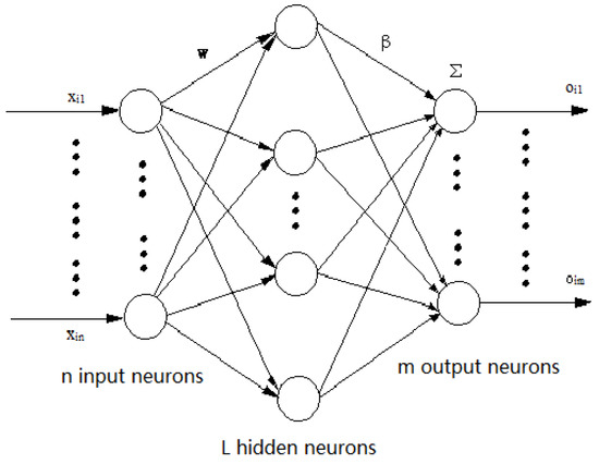
Figure 1.
Kernel extreme learning machine (KELM) model structure.
For any given set of N samples (xi, ti), as shown in Figure 1, where xi = [xi1, xi2, …, xin]T ∈ Rn, ti = [ti1, ti2, …, tin]T ∈ Rm, the number of neurons in the hidden layer is L, and the activation function of the hidden layer is g(x), so the mathematical expression of the hidden layer feed forward neural network is:
where, wi = [wi1, wi2, …, win]T is the weight between the i-th hidden layer neuron and the input neuron; βi = [βi1, βi2, …, βim]T is the weight between the i-th hidden layer neuron and the output neuron; bi represents the offset value of the i-th hidden layer neuron, wi·xj represents the inner product of wi and xj, and oj represents the output vector.
For a single hidden layer feedforward neural network, it can approach the N sample collections with zero error, i.e.,
When existing βi, wi and bi make Equation (3) set up,
The above expression can be abbreviated as:
where, H = {hij}(i = 1, 2, …, N; j = 1, 2, …, L), H is the output matrix of the hidden layer of the single hidden layer feed forward neural network. T is the respected output of the hidden layer of the single hidden layer feed forward neural network. tj is an element in the matrix T. So if the oj can infinitely close to the tj, that means the predicted effect of extreme learning machine model is very close to the true value.
The extreme learning machine trains the network by minimizing the training error and minimizing the norm of the output weight, which is min‖β•h(xi) − ti‖2 and min‖β‖. Here, β is the weight vector connecting the hidden layer neurons and the output neurons, h(xi) is hidden layer core mapping. From the point of view of standard optimization theory, the above problem can be solved by a simplified constrained optimization problem, and the above target can be rewritten as:
Restrictions:
where, C is the regularization coefficient and ξi is the training error.
According to the Karush–Kuhn–Tucker condition, the above problem can be transformed into the optimization problem of the following Equation:
where ηi is a Lagrangian operator, the above optimization problem can be equivalent to:
where η = [η1, η2, …, ηN]T. For the training samples, substituting Equations (8) and (9) into Equation (10), respectively,
According to the Mercer condition, construct a kernel function to instead of HHT, so
The output of the kernel function extreme learning machine can be expressed as,
2.2. Kernel Extreme Learning Machine Solution Steps
The kernel extreme learning machine algorithm calculation flow is shown in Figure 2. Data such as network node voltage, distributed generation power output and electric vehicle charging power are obtained through distribution power flow calculation, and are used as training data. PDG and PEV are used as input of the kernel extreme learning machine model, and U is used as output, to train the kernel extreme learning machine.
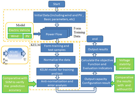
Figure 2.
Flowchart of KELM algorithm. (PV: Photovoltaic; EV: Electric Vehicle; SVM: Support vector machine)
Through training, the kernel extreme learning machine model is established, and the root mean square error is calculated as an evaluation index for judging the prediction accuracy, that is,
where, RMSE represents the root mean square error, y(i) represents the actual value, y*(i) represents the predicted value, N is the number of samples. The smaller the RMSE value, the better the prediction accuracy.
The improved voltage stability evaluation index [17], Ivse is used to reflect the influence with different distributed generation capacity configuration scheme on network voltage. The voltage stability index is based on the extreme conditions of the power flow solution to determine the system voltage stability. This index can reflect the area and the node in the system where voltage collapse is most likely to happen [18]. The smaller the index value, the more stable the network voltage. The index Equation is as follows:
where, Q represents the network reactive loss, Z represent the equivalent impedance, and U represents the node voltage.
3. Math Models of Wind, Photovoltaic and Electric Vehicle
3.1. Wind and Photovoltaic Model
Generally, the distribution of wind speed is considered to be a two-parameter Weibull distribution, and the probability density function [19] can be expressed by,
The output power of the fan changes with the change of the wind speed, and the output can be expressed as,
where, c and k are the two parameters of the Weibull distribution; v is the actual wind speed; vci is the cut in wind speed; vco is the cut off wind speed; vn is the rated wind speed; Pw is the rated power of the fan.
At the same time, the solar light intensity can also be considered to approximate the Weibull distribution, and its probability density function [20] can be expressed as,
The output power of a photovoltaic cell varies with the intensity of the light, and the output can be expressed as,
where, s is the light intensity, sn is the light intensity under the rated power output, and Psn is the rated output of the photovoltaic cell.
3.2. Electric Vehicle Model
The charging demand of an electric vehicle is usually related to the battery characteristics of the vehicle, the travel habits of the owner, and the charging mode. The battery characteristics are usually expressed by the state of charge (SOC), and the charging mode is mainly divided into fast and slow charging mode. Combined with the travel habits of car owners, private cars are the main research object in this paper. Two indicators are introduced to express the charging demands of electric vehicles: the location and capacity of the charging stations.
The location information can reflect the convenience and the charging mode of the vehicle owner. The locations of the charging stations are divided into two types, one is the commercial or tourism centers, which usually adopt the fast charging mode, and the other is the residential centers or enterprises and institutions, which usually adopt the slow charging mode. The capacity information can reflect the rationality and economy of the charging station. If the capacity and number of charging piles are too large, the investment cost of the charging station will be too high. If the capacity and the number of charging piles are too small, the charging demand cannot be satisfied. Therefore, it is important to properly plan and design the location and capacity of electric vehicle charging stations.
According to the 2017 global traditional energy power report [21], per capita annual electricity consumption in 2017 was about 4309 kWh, which can be used to estimate the population within the selected network’s power supply area. Set the population within the power supply area as Ps, the annual electricity consumption within forecasting area as Aec, and the per capita electricity consumption as Pcec, the Equation for Ps is as follows:
According to the calculated number of cars per 100 people in developed regions, 32 vehicles/100 people, electric vehicle occupancy was calculated to be 40%. Among this, the fast charging mode accounted for 20% of the total number of electric vehicles, and the slow charging mode accounted for 80%. The availability rate of electric vehicles with fast charging modes is setting as 0.6. The slow charging mode vehicles, the rate is setting as 0.3. Thus, an estimated value of the charging powers of the electric vehicles is derived:
where, PEVin represents one electric vehicle charging power. PEVC represents the charging power of all the electric vehicles in the network.
So according Equations (5)–(7), using the actual data from some wind field and photovoltaic power stations, the power ranges of fast and slow charging modes needed by the electric vehicle can be derived, and the charging power can be derived by a Monte Carlo method. The electric vehicle charging power obeys a normal distribution. The distribution curve of electric vehicle charging power is presented in Figure 3. The X-axis indicates the charging power of electric vehicle and the Y-axis indicates the probability value of the electric vehicle charging power, and this value has no unit. μ represents the average value of the electric vehicle charging power when its probability value is the largest, and its unit is MW.
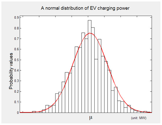
Figure 3.
The distribution curve of electric vehicle (EV) charging power.
3.3. Objective Function and Constraints
3.3.1. Objective Function
An opportunity constrained programming method is used to set up an objective function with the lowest active power loss and investment cost, considering the influence of the distributed generation access.
The total investment of power grid projects generally consists of static and dynamic investments. During the power grid planning process, the investment estimates used for economic evaluation generally refer to static investments. Static investments include project construction costs, equipment purchase costs, other construction costs, and basic reserve fees. Therefore, under the premise of considering the economic evaluation and technical indicators, the objective function with the smallest total investment cost and network active loss was constructed:
where C is the total investment cost of the system; CDG is the investment cost of each distributed generation; CEV is the investment cost of each electric vehicle charging station; Ploss is the network loss; I is the current, and R is the equivalent resistance; m represents the access number of distributed generation or electric vehicle.
The unit capacity method was used to calculate the system investment cost. Using the actual wind and photovoltaic project investment as an example, the following comprehensive cost indicators which contain investment and operation costs are obtained. The wind power was about 8.02 RMB/w, and the photovoltaic power was about 7.91 RMB/w. The charging station costs mainly consist three parts: infrastructure, power distribution facility, and operating costs. According to the calculation method mentioned in [22], the comprehensive cost can be derived as follows:
where, C is the investment and operation cost; si is the scale of the project; pi is the unit’s comprehensive cost estimation index of the project.
3.3.2. Equivalent Constraint
An equality constraint is derived from the power flow Equation as follows,
where, P and Q represent the active and reactive power; PDG and QDG represent the active and reactive power injected by distributed generation; PL and QL represent the active and reactive load; U represents the node voltage; PEV represents the electric vehicle charging power.
3.3.3. Inequivalent Constraint
Considering the impact of the distributed generation and electric vehicle access, the voltage of each node was limited as follows:
where Umin is the lower limit value, and Umax is the upper limit of the node voltage. The distributed generation access capacity is constrained by the limit,
where SDG is the installation capacity of the distributed generation, and SDGmax is the maximum value. The electric vehicle access capacity is defined as follows:
where SEV is the capacity of the electric vehicle, and SEVmax is the maximum allowable installation capacity.
4. Simulations
4.1. Parameter Setting
The IEEE33 node power distribution system structure diagram is shown in Figure 4. The relevant parameters can be found in Table A1 of the Appendix A. Based on actual measured data of a project, the wind speed obeys a Weibull distribution with k = 5.8 and c = 16. The illumination intensity obeys a Weibull distribution with k = 0.45 and c = 9.18. The number of data samples was set to 1000.
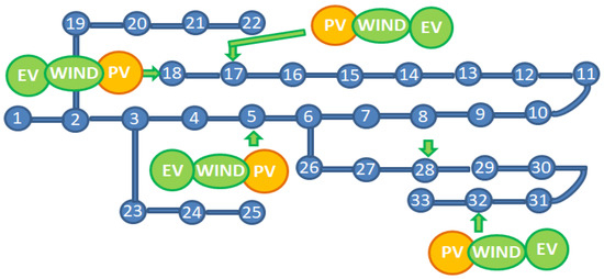
Figure 4.
IEEE 33 distribution network structure.
The access locations of wind, photovoltaic and electric vehicle are shown in Figure 4. With different combinations, there can be at least three cases for distributed generation. Case 1 represents one wind or one photovoltaic accessing one node; case 2 represents one wind and one photovoltaic access into two nodes, and case 3 represents wind and two photovoltaic access into three nodes, respectively. The candidate nodes for accessing wind, photovoltaic and electric vehicle are selected as follows: node 5, node 17, node 18, node 28 or node 32.
4.2. Kernel Extreme Learning Machine Prediction Accuracy Verification
Figure 5 shows the average root mean square error value of kernel extreme learning machine under different access modes. The abscissa represents the different access modes of the distributed generation (shows in Appendix A Table A2), and the ordinate represents the value of the root mean square error (RMSE). It can be seen that the RMSE curve of the kernel extreme learning machine was relatively flat, and its average value is 0.04; the change of support vector machine is relatively large, and its average value is 0.062. A flatter curve corresponds to a smaller RMSE value, indicating that the prediction accuracy is better. Therefore, the kernel extreme learning machine prediction was better than that of the support vector machine.
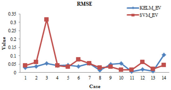
Figure 5.
Changes of root mean square error (RMSE).
To verify the feasibility and reasonability of kernel extreme learning machine, comparing the results of kernel extreme learning machine with and without electric vehicle. The calculation results of the kernel extreme learning machine without electric vehicle are given in Table 1.

Table 1.
Results of kernel extreme learning machine without electric vehicle; (DG: distributed generation).
It can be seen from Table 1 that as the number of distributed generation increases, the active power loss increases. As the distributed generation access location and capacity change, it will cause changes in network power flow. The larger the distributed generation access capacity, the greater the impact on the network power flow distribution. So the active loss increases with the access of distributed generation. The access node is listed behind the distributed generation capacity with brackets.
Table 2 is the results with electric vehicle connecting, and the average capacity of the electric vehicle is 0.285 MW at node 32. For convenience of comparison, the electric vehicles are not included in the total investment cost.
Table 2.
Results of kernel extreme learning machine with electric vehicle.
It can be seen from Table 2 that when electric vehicle access is taken into account, the capacity of wind and photovoltaic increases, while the active power loss decreases. So the electric vehicle access is beneficial to the access of distributed generation and helpful to reduce active power losses.
On the other hand, the results of kernel extreme learning machine are compared with that of a support vector machine. With similar access capacities, the total investment costs are compared. The total investment cost obtained by the kernel extreme learning machine is reduced, with an average decrease of 0.8%, and the active loss was reduced by an average of 28%. In the calculation time, the support vector machine average calculation time was about 22.6 s, and the kernel extreme learning machine is about 16.9 s. Analyzing the reasons, in addition to the inherent calculation time required for the power flow calculation, the kernel extreme learning machine needs time on the millisecond level, while the support vector machine requires 3–5 s.
The model mainly utilizes kernel extreme learning machine’s non-linear approximation ability and generalization performance to approximate the non-linear relationship between the node voltage and the distributed generation power. The above analysis shows that the kernel extreme learning machine is better than the support vector machine in terms of calculation speed and prediction accuracy. And its calculation results are feasible and reasonable.
4.3. Voltage Stability Evaluation Index
To further verify the rationality of the distributed generation and electric vehicle capacity selection results given by the kernel extreme learning machine, the voltage stability evaluation index (Ivse) is introduced to evaluate. The value of Ivse for all the nodes before installing wind and photovoltaic are mentioned in Figure 6. The X-axis indicates the node number and the Y-axis indicates the value of the Ivse indicator. Table 3 shows the changes in the indicators with different distributed generation access modes without electric vehicles.
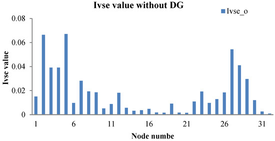
Figure 6.
The voltage stability evaluation index (Ivse) initial value without DG. (DG: distributed generation).
Table 3.
Index value of Ivse without electric vehicle.
Ivse_o represents the original Ivse value when the distributed generation is not connected. Ivse_case1 represents the index value when distributed generation is connected under case1, so as Ivse_case2 and Ivse_case3. As shown in Table 3, the Ivse value is gradually decreased compared with Ivse_o. According to the definition of the Ivse, that means the corresponding node voltage stability is improved. So the distributed generation access is helpful to improve the voltage stability.
Ivse_case n&ev is the value of Ivse when distributed generation and electric vehicles are both connected. As shown in Table 4, the Ivse value decreases as the number of distributed generation and electric vehicles increase. So through comparing the changing trends of Ivse, the access of distributed generation and electric vehicles are beneficial to improve the voltage stability.
Table 4.
Index value of Ivse with electric vehicle.
4.4. Voltage Stability Analysis
As the access number of distributed generation and electric vehicle is increasing, it will have a great impact on the stability of the network voltage. Therefore, it is necessary to analyze the effects on the network voltage distribution under different access modes of distributed generation and electric vehicle.
In Figure 7a–c, the dark blue curve in the figure corresponds to V_noDG, define as the initial voltage distribution of the network without distributed generation and electric vehicle. The red and green curves correspond to V_KELM_nDG and V_SVM_nDG, respectively define as the voltage distribution of the network when only distributed generation are connected, where n = [1, 2, 3] representing case1, case2, case3 respectively. The light blue and purple curves correspond to V_KELM_nDG&EV and V_SVM_nDG&EV respectively define as the voltage distribution when distributed generation and electric vehicles are connected at the same time.
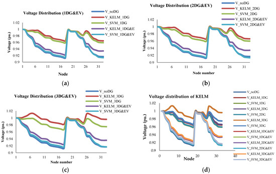
Figure 7.
Voltage distribution curves by comparing KELM with SVM under different DG&EV configuration scheme; (a) DG access in case1 and with or without EV; (b) DG access in case2 and with or without EV; (c) DG access in case3 and with or without EV; (d) voltage profile of KELM with different DG access modes and with or without EV.(DG: Distributed generation; EV: Electric vehicle)
Figure 7a–c, shows the change of the voltage gained by the kernel extreme learning machine and support vector machine methods, with different distributed generation access modes and with or without electric vehicle. The voltage amplitude increases with the distributed generation access capacity. This indicates that the access of the distributed generation is beneficial for increasing the network voltage level. Meanwhile, by comparing the results obtained by the support vector machine, the voltage distribution curve given by kernel extreme learning machine is better.
On the other hand, when considering the electric vehicle access, by comparing the voltage distribution curves before and after electric vehicle access, shown in Figure 7d. After distributed generation and electric vehicle access, the voltage distribution is better than the original voltage level (V_noDG&EV). So the distributed generation and electric vehicle access is helpful to improve the voltage stability.
5. Discussion
Through the above comparison and analysis, it was found that distributed generation and electric vehicle access have a great influence on improving the network voltage stability, and the characteristic of electric vehicle charging also has a positive effect on the network to absorb distributed generation.
In addition, to further illustrate the effectiveness of the distributed generation and electric vehicle capacity selection results given by the kernel extreme learning machine, the results are compared with those obtained by the support vector machine, particle swarm optimization algorithm and genetic algorithm method, as shown in Table 5.
Table 5.
Comparison of kernel extreme learning machine with other optimization methods. (PSO: Particle swarm optimization; GA: Genetic Algorithm).
In order to make the results are comparable, focusing on the distributed generation sizing problems without electric vehicles, and with the same objective function, that is the active power loss is minimum, and the same access location, to compare the results of the kernel extreme learning machine with the particle swarm optimization algorithm, genetic algorithm and support vector machine.
From Table 5, we can see, the capacity of distributed generation obtained by kernel extreme learning machine is larger than particle swarm optimization algorithm and support vector machine, while the active power loss is smaller. So through this comparison, we believe that the results obtained by the kernel extreme learning machine are better.
6. Conclusions
In view of the fundamental changes in the planning and operation characteristics of distribution networks caused by the large-scale access of wind and photovoltaic power generations and electric vehicles, the kernel extreme learning machine is used to build the capacity selection model. By training the model, the capacity selection results of distributed generation that satisfies the objective function is obtained by the kernel extreme learning machine. The main conclusions are as follows:
- (1)
- The model constructed by the kernel extreme learning machine can effectively approximate the non-linear relationship between the wind and photovoltaic power output and network node voltage, when considering the electric vehicle charging characteristic.
- (2)
- The kernel extreme learning machine calculation speed is fast, its average training time is 23.3 milliseconds. Its prediction accuracy is better. Through the comparison of the root mean square error with support vector machine, its average value is decreased by 35%.
- (3)
- Through comparison with the support vector machine, particle swarm optimization algorithm and genetic algorithm, the distributed generation capacity selection results given by the kernel extreme learning machine are reasonable, and are beneficial for improving the voltage stability.
- (4)
- The access of electric vehicles is beneficial to increase the distributed generation access capacities. By calculating the access capacity ratio of distributed generation and electric vehicles by the kernel extreme learning machine, it is possible to increase the distributed generation access capacity up to 20%–40%.
However, given the comparison and analysis above, further study is still needed. For example, with the same objective function, the results of distributed generation capacity selection model is reasonable, and it is better than the particle swarm optimization algorithm or genetic algorithm, but as the amount of training data increased, the computational speed complexity increased and the calculation accuracy decreased. Therefore, a future study needs to optimize certain parameters, so that the kernel extreme learning machine can obtain a better distributed generation configuration strategy.
Author Contributions
Methodology, J.T.; software, J.T., Y.X.; validation, Z.Y., J.T. and Y.X.; formal analysis, J.T., Y.X.; data curation, J.T., Z.Y.; writing—original draft preparation, J.T.; funding acquisition, J.T., Z.Y.
Funding
This research was funded by the National Key Research and Development Program of China under Grant, grant number 2016YFB010190.
Conflicts of Interest
The authors declare no conflict of interest.
Appendix A
Table A1.
Data for the IEEE 33-bus radial distribution system [25].
Table A2.
Different access modes of distribution generations.
References
- Erdinc, O.; Tascikaraoglu, A.; Paterakis, N.G.; Dursun, I.; Sinim, M.C.; Catalão, J.P.S. Optimal Sizing and Siting of Distributed Generation and EV Charging Stations in Distribution Systems. In Proceedings of the 2017 IEEE PES Innovative Smart Grid Technologies Conference Europe (ISGT-Europe), Torino, Italy, 26–29 September 2017; pp. 1–6. [Google Scholar]
- Mahmoud Pesaran, H.A.; Huy, P.D.; Ramachandaramurthy, V.K. A review of the optimal allocation of distributed generation: Objectives, constraints, methods, and algorithms. Renew. Sustain. Energy Rev. 2017, 75, 293–312. [Google Scholar] [CrossRef]
- Ehsan, A.; Yang, Q. Optimal integration and planning of renewable distributed generation in the power distribution networks: A review of analytical technique. Appl. Energy 2018, 210, 44–59. [Google Scholar] [CrossRef]
- Asimakopoulou, G.E.; Hatziargyriou, N.D. Evaluation of Economic Benefits of DER Aggregation. IEEE Trans. Sustain. Energy 2018, 9, 499–510. [Google Scholar] [CrossRef]
- Qi, C.; Dong, X.F.; Tong, J. Optimization Planning of Integrated Electricity-Gas Community Energy System Based on Coupled CCHP. Power Syst. Technol. 2018, 42, 2456–2466. [Google Scholar]
- Baghayipour, M.R.; Hajizadeh, A.; Shahirinia, A.; Chen, Z. Dynamic Placement Analysis of Wind Power Generation Units in Distribution Power Systems. Energies 2018, 11, 2326. [Google Scholar] [CrossRef]
- Lina, W. Locating and Sizing of Distributed Generations in Distributed Network Considering Uncertainties. Distrib. Energy 2018, 3, 23–28. [Google Scholar]
- Xiufan, M.; Chao, W.; Xiao, H.; Ying, L.; Hao, W. A Two Layer Model for Electric Vehicle Charging Optimization Based on Location Marginal Congestion Price. Power Syst. Technol. 2016, 40, 3706–3714. [Google Scholar]
- Wei, W.; Yue, C.; Feng, L.; Shengwei, M.; Fang, T.; Xing, Z. Stackelberg Game Based Retailer Pricing Scheme and EV Charging Management in Smart Residential Area. Power Syst. Technol. 2015, 39, 939–945. [Google Scholar]
- Haidar, A.M.A.; Muttaqi, K.M. Behavioral characterization of electric vehicle charging loads in a distribution power grid through modeling of battery chargers. IEEE Trans. Ind. Appl. 2015, 52, 483–492. [Google Scholar] [CrossRef]
- Shafiee, S.; Fotuhi-Firuzabad, M.; Rastegar, M. Investigating the impacts of plug-in hybrid electric vehicles on power distribution systems. IEEE Trans. Smart Grid 2013, 4, 1351–1360. [Google Scholar] [CrossRef]
- Huang, G.B.; Zhu, Q.Y.; Siew, C.K. Extreme learning machine: theory and applications. Neurocomputing 2006, 70, 489–501. [Google Scholar] [CrossRef]
- Huang, G.B.; Bai, Z.; Kasun, L.L.C.; Vong, C.M. Local receptive fields based extreme learning machine. IEEE Comput. Intell. Mag. 2015, 10, 18–29. [Google Scholar] [CrossRef]
- Dong, H.; Li, M.X.; Zhang, S.Q.; Han, L.Q.; Li, J.F.; Su, X.S. Short-term power load forecasting based on kernel principal component analysis and extreme learning machine. J. Electron. Meas. Instrum. 2018, 32, 188–193. [Google Scholar]
- Huang, N.T.; Chen, H.J.; Lin, L.; Qi, J.J. Mechanical Fault Diagnosis of High Voltage Circuit Breakers Based on S-transform and Extreme Learning Machine. High Volt. Appar. 2018, 54, 74–80. [Google Scholar]
- Chen, Y.R. Application of Intelligent Algorithm Based on Genetic Algorithm and Extreme Learning Machine to Deformation Prediction of Foundation Pit. Tunn. Constr. 2018, 38, 941–947. [Google Scholar]
- Tu, J.J.; Yin, Z.D.; Xu, Y.H. Study on the Evaluation Indicator System and Evaluation Method of Voltage Stability of Distribution Network with High DG Penetration. Energies 2018, 11, 7993. [Google Scholar]
- Jiang, B.; Wu, J.; Feng, L.; Wu, K.H.; Liang, R.; Yang, B.; Li, X.; Chen, H.J. Research on static voltage stability calculation indicator of active distribution network with distributed generation. J. Electron. Meas. Instrum. 2017, 31, 885–891. [Google Scholar]
- Zhang, Z.; Li, G.; Wang, J. Probabilistic evaluation of voltage quality in distribution networks considering the stochastic characteristic of distributed generators. Proc. CSEE 2013, 33, 150–156. [Google Scholar]
- Evangelopoulos, V.A.; Georgilakis, P.S. Optimal distributed generation placement under uncertainties based on point estimate method embedded genetic algorithm. IET Gener. Transm. Distrib. 2014, 8, 389–400. [Google Scholar] [CrossRef]
- Li, Z.K.; Tian, Y.; Dong, C.M.; Fu, Y.; Zhang, J.W. Distributed Generators Programming in Distribution Network Involving Vehicle to Grid Based on Probabilistic Power Flow. Autom. Electr. Power Syst. 2014, 38, 60–66. [Google Scholar]
- Yao, W.F.; Zhao, J.H.; Wen, F.S.; Xue, Y.S.; Dong, Z.Y. Coordinated Planning for Power Distribution System and Electric Vehicle Charging Infrastructures. Autom. Electr. Power Syst. 2015, 39, 10–18. [Google Scholar]
- Aman, M.M.; Jasmon, G.B.; Bakar, A.H.A.; Mokhlis, H. A new approach for optimum simultaneous multi-DG distributed generation units placement and sizing based on maximization of system loadability using HPSO (hybrid particle swarm optimal) algorithm. Energy 2014, 66, 202–215. [Google Scholar] [CrossRef]
- Moradi, M.H.; Tousi, S.M.R.; Abedini, M. Multi-objective PFDE algorithm for solving the optimal siting and sizing problem of multiple DG sources. Int. J. Electr. Power Energy Syst. 2014, 56, 117–126. [Google Scholar] [CrossRef]
- Tu, J.J.; Xu, J.H.; Yin, Z.D. Data-Driven Kernel Extreme Learning Machine Method for the Location and Capacity Planning of Distributed Generation. Energies 2019, 12, 109. [Google Scholar] [CrossRef]


© 2019 by the authors. Licensee MDPI, Basel, Switzerland. This article is an open access article distributed under the terms and conditions of the Creative Commons Attribution (CC BY) license (http://creativecommons.org/licenses/by/4.0/).