1. Introduction
The problem of corrosion of steel materials is generally known. In general, great attention has been paid to efforts to eliminate its effects. Our research aims to eliminate the effects of atmospheric corrosion. The anticipated load according to EN ISO 9223 assumes stress corrosion conditions of corrosion grade C3 (medium) to C4 (high, corresponding to wet areas, industrial zones, ports, etc.).
There are a number of known methods for protecting metal surfaces against moisture and corrosive vapors as well as methods that utilize physical or chemical methods in terms of corrosion protection.
Simple procedures and guidelines for protection can be found in the use of corrosion inhibitors, which represent an inexpensive and effective alternative to traditional protection, cathodic protection, incorporation of suitable alloys, efficient process control, reduction of alloy impurities and use of surface treatment techniques, etc. according to Chigondo [
1] and also Lgaz et al. [
2]. Kashif and Ahmad [
3] described the principle procedure where nanoparticles of oil are deposited as a protective layer against corrosion by their dispersion, standard methods have already been applied, such as weight loss, electrochemical impedance spectroscopy and potentiodynamic polarization to determine the corrosion resistance performance.
Pourhashem et al. [
4] studied the enhancement of corrosion protection through solvent-based epoxy–graphene oxide application. Research results presented by Zhang et al. [
5] showed that the fabricated superhydrophobic film had excellent corrosion resistance and excellent corrosion protection efficiency.
Zavareh et al. [
6] wrote about methods of coating the surface with two new advanced ceramic composite materials. Mallozzi and Kehr [
7] dealt with cases where it is necessary to combine mechanical and chemical resistance. The methods of non-destructive testing solutions for monitoring and inspection of pipelines and pressure vessels to the oil and gas industry were discussed by Shameli [
8]. New scientific work on green polymers and corrosion inhibitors were analyzed by Chen [
9]. It is gradually used in industrial processes to protect carbon steel against corrosion in the solution environment. For mild steel corrosion protection, Bustos-Terrones [
10] recommended composite material SBA-15 (silicon oxide) as a mild steel corrosion inhibitor. Lorza [
11] in his work focused on optimizing the use of zinc electroplating on steel material surfaces. Barrera [
12] analyzed the new coatings on cast iron. Special attention was paid to low-maintenance methods of protection.
An interesting article from Božek [
13] may be an inspiration for a pragmatic analysis of the solution of a previously unidentified problem and the way of designing the calculation procedure in general.
However, the most important parameter is the resulting layer thickness applied to the inner surface of the pipe. One possible way is the optical sensing principle, which is the desired contactless measurement method. It is precisely this subject that can be found in the description of this interesting method of sensing similar quantities, as explained in the article by Krehel [
14].
It is necessary to achieve a high level of reliability and productivity with a well-established and functioning production system. Turygin [
15] deals with reducing the number and time of layups and increasing the period of effective operation of a mechatronic system to carry out predictive recovery works. This method is well applicable to the above-mentioned method.
In practice, the protection of the inner surface of long tubes with a small diameter (hereinafter referred to as “slim tubes”) is solved by a method of immersing the entire tubes into chemical fluid in order to provide protection against corrosion, e.g., “Anticorid DFV 2001” (hereinafter “oil”) from Fuchs Oil Corp. Ltd. (Gliwice, Poland) [
16]. After a sufficient period of time, the tubes are removed from the bath and allowed to drip for 24 h followed by manual wiping and cleaning of oily surface film. This cleaning is a physically demanding, time-consuming, dangerous and unhygienic practice. Even the greatest effort to thoroughly clean the oily outer surface of the pipes and the leaking oil inside the pipes, is the result of practice. This seems to be an unsuitable method and it is necessary to look for better ways to improve how to apply oil to the inner surface of the slim tubes.
2. Numerical Calculation of Oil Dispersion Flow in Flowing Air
To obtain a comprehensive view of the influence of the velocity of the airflow on the change in the average surface density of the oil film applied to the inner surface of the slim tubes, calculations were performed for the range of velocities at which good conformity with the experimental results was obtained. The purpose of numerical simulation is to point out the possibility of eliminating experimental measurements by applying numerical methods to other shapes and dimensions of the coating surface applied by using dispersed oil. However, the problem is the considerable dependence of the numerically calculated area density of the applied oil on the large number of input parameters, the feed rate of the mixture, the roughness of the slim tube, or the angle of inclination of the input velocity towards the axis of the slim tubes.
Jablonská [
17] characterized the dynamic flow behavior in oil piping, where a mathematical model of dynamic behavior was obtained using Matlab SimHydraulics software. Križan [
18] also applied this mathematical model to the process of biomass compaction. The aim of this model is to determine the impact of process parameters, its usefulness when applied to oil flow.
Leporini M. et al. [
19], in their study, dealt with a similar issue of transporting small particles of sand in piping systems using one-dimensional dynamic multiphase code. Jing J. et al. [
20] in their publication focused on an experimental and numerical study in order to determine the amount of an anticorrosion inhibitor applied by injecting an appropriate volume into a horizontal pipeline. They also came to the conclusion of a reduced concentration of liquid at the top of the pipeline.
The following section provides a detailed view of the mathematical formulation of multiphase flow which will be used in numerical calculation.
2.1. Mathematical Formulation
Ansys CFX 19.1 software was used for the numerical calculation of the multiphase fluid flow represented by the oil fraction in the flowing air. Software solves the conservation equations for momentum, mass and energy by the finite volume formulation. The equations are expressed in terms of the Cartesian coordinate system.
Continuity equation for multiphase non-homogeneous flow without mass sources and mass flow rate per unit volume from phase
β to phase
α is as follows:
where
rα is the volume fraction of phase
α,
ρα is the density of the
α- phase as the phase of the fluid,
t is time, and
Uα is the velocity of the phase
α as the phase of the fluid. The momentum conservation equation is given by:
where
p is the static pressure,
µα is dynamic viscosity,
Mα describes the interphase forces acting on the
α phase due to the presence of other phases. An interphase drag with drag coefficient
CD = 0.44 was used in Interphase Momentum Transfer Models. Lift coefficient
CL = 0.5 was defined for the lift force. The wall lubrication force was activated according to the numerical solution of the two-phase flow which acts on the oil fraction and is described by:
where
Cwl is the wall lubrication coefficient (1),
ρq is the primary phase density,
αp is the oil volume fraction,
is the phase relative velocity component tangential to the wall surface (m·s
−1), and
is a normal unit pointing away from the wall.
Antal et al. Model [
21] was used to calculate the wall lubrication coefficient:
where
Cw1 = −0.01 and
Cw2 = 0.05 are non-dimensional coefficients,
db is the particle diameter, and
yw is the distance to the nearest wall.
The homogeneous
k-
ω SST (Share Stress Transport) turbulence model was used for the numerical calculation of the multiphase flow with the corresponding
k- and
ω- equations containing the buoyancy effects:
where
k is the turbulent kinetic energy,
ω is specific dissipation rate, µt is turbulent dynamic viscosity calculated by (7),
x is the space coordinate, and
Pk is the shear production of turbulence.
The coefficients
σk3 and
σω3 are calculated by a linear combination of the respective coefficients according to the following Equations (8) and (9).
The blending functions (10) are critical to the success of the method. Their formulation is based on the distance to the nearest surface and on the flow variables:
where
y is the distance to the nearest wall,
ν is the kinematic viscosity. These mathematical dependencies and parameters are described in detail in the literature [
22].
2.2. Computational Domain and Boundary Conditions
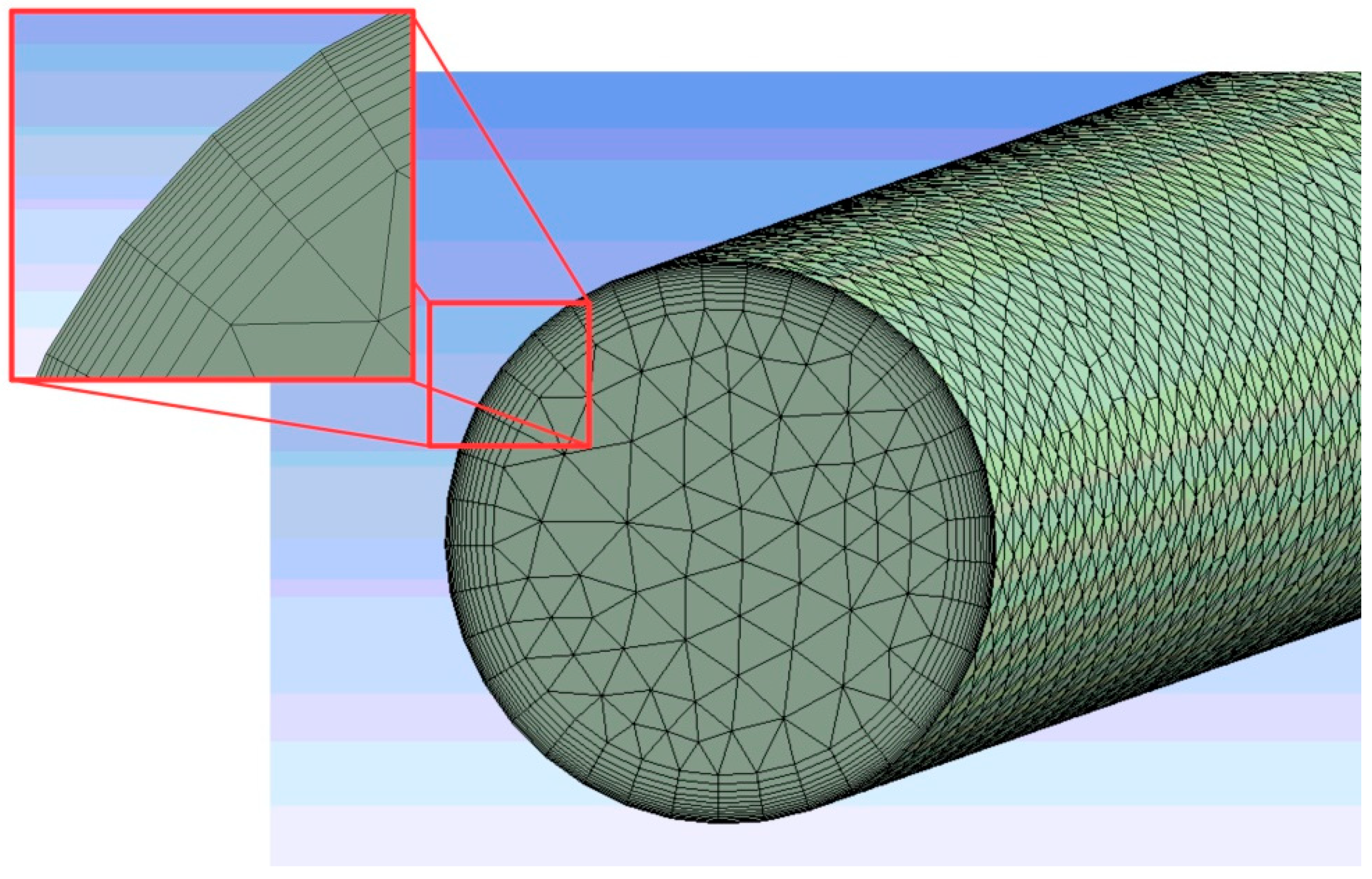
A three-dimensional numerical simulation was chosen for this study. Numerical calculation was carried out for three different pipe diameters (35, 25 and 15 mm), which were identical to the pipe diameter during the experiment. The pipeline had a length of 6 m with respect to isothermal flow without the need for heat transfer and it consists of only one domain representing air with an oil dispersion. In order to simplify the evaluation results of the analysis, the domain was divided into 30 volumetric subdivisions (0.2 m/element). Each of the areas created for specific geometry and flow velocity was divided by the network into the final number of the tetrahedron volume elements. Modeling the fluid velocity near the pipe wall in the boundary layer was ensured by densifying the mesh at the wall, wherein the thickness of the first element was determined from the selected dimensionless distance value of
y+ = 1.
Figure 1 is a view of a part of the mesh formed at the inlet of the pipe for pipe diameter of 35 mm and a flow rate of 5 m∙s
−1, wherein the thickness of the first element at the wall is 0.076 mm. The number of mesh elements after the boundary layer thickness is 12 with an increase of 1.2. With an average mesh size of 5 mm, the total number of elements of the selected geometry is 3.28 mil.
A numerical simulation of the airflow with an oil dispersion of an average oil particle size of 0.2 µm was from a physical point of view designed as isothermal multi-phase turbulent airflow with a temperature of 10 °C, using the SST turbulence model. Air with continuous fluid and oil as dispersed fluid morphology was the carrier gas and a buoyancy model with a gravitational acceleration value of 9.81 m·s−2 was included in the solution. A multi-phase inhomogeneous flow model with homogeneous turbulence calculation was employed. The domain reference pressure was determined at 1 atm according to the conditions of the experiment. Within the initialization conditions (at time τ = 0 s), the zero velocity of the flowing fluid was defined in the entire volume, as well as zero relative static pressure and zero volume fraction of oil.
The input boundary condition was set with a defined subsonic air velocity with an oil fraction, based on the set value of the input intensity of the turbulence at the level of 10%. The oil mass flow rate based on experimental knowledge is 4.67·10
−4 kg·s
−1. The dispersed oil particles flow at the selected speed according to the boundary condition at the pipe entry, wherein oil volume fraction at the inlet is given by the following formula:
where
roil is oil volume fraction of oil (1),
Voil—oil volume (m
3),
Vair—air volume (m
3),
Qm,oil—oil flow rate (kg∙s
−1),
ρoil—oil density (kg∙m
−3),
d—pipe diameter (mm),
v—airflow velocity (m∙s
−1). Volume fraction of air is subsequently calculated as (1 −
Φoil). At the outlet of the duct, a boundary condition was specified with an average relative static pressure of 0 Pa by averaging pressure using the Average Over Whole Outlet method. A zero fluid velocity (No Slip Wall) with an absolute surface roughness of 0.03 mm is set on the cylindrical surface of the pipe.
2.3. Time and Solver Settings
The calculation was carried out as time-dependent with a total time of 15 s and a time step of 0.05 s. A maximum of 40 iterations were used with required target residuals of 10−5 along with the residual type of RMS (Root Mean Square). The evaluation of the investigated parameters was subsequently carried out in the final time of 15 s.
2.4. Results
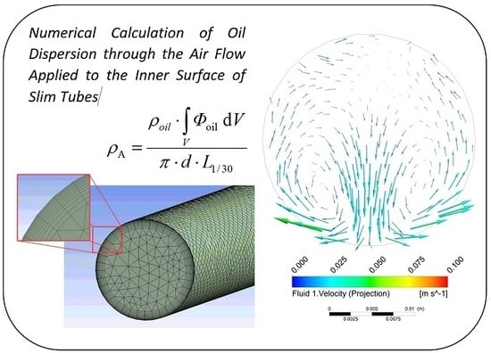
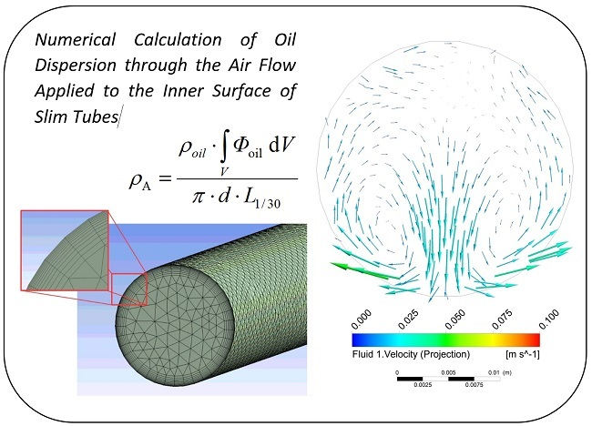
Three simulations were performed at 4, 4.7 and 5 m/s for a 35 mm pipe diameter. For individual velocities, the change of the mesh quality was calculated based on the following formula; thicknesses of the first element compared to the size of the mesh at the wall. After numerical calculation, the quantities of oil in each volume section with a length of 0.2 m were evaluated and subsequently converted to the area density of oil in relation to:
where
ρA is the areal oil density (kg·m
−2),
dV is the elemental volume of the domain geometry (m
3),
L1/30 is the length of 1/30 of the pipe (0.2 m) (m).
Figure 2 shows the flow rate of the oil for three different speeds together with the data measured for a diameter of 35 mm.
It is clear from the plots that at speeds of up to 4.7 m/s, the coverage of the inner surface of the pipe in the second half of its length is almost zero. At higher speeds, the resistance force acting on the oil particles overtakes the flow of air against gravitational force, and the particles are carried and distributed over the entire length of the pipe. At a speed of 5 m/s, the results of the numerical calculation are in very good agreement with the results of the experiment. At a speed of 5 m/s, a minimum coverage of 1.4 g·m−2 of oil film is provided over the entire length of the pipe.
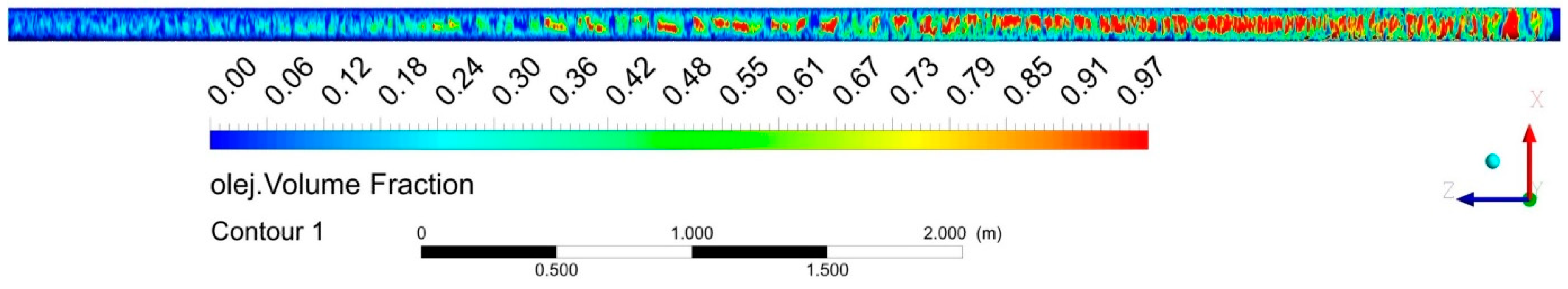
Figure 3 shows the volume of oil at the surface of the pipe over its full length at a speed of 4 m/s measured volume fraction scale obtained at 15-s intervals. For comparison,
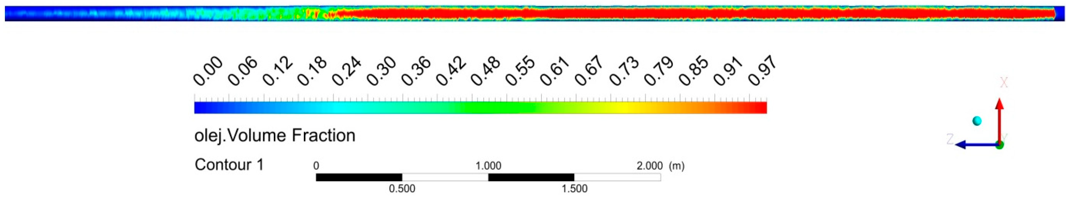
Figure 4 shows the volume of oil over its full length at a speed of 5 m/s.
Figure 4 shows that the oil fraction covering the pipe over its full length at a speed above 5 m·s
−1 is more pronounced over its entire length and contributes to achieving the minimum required oil density.
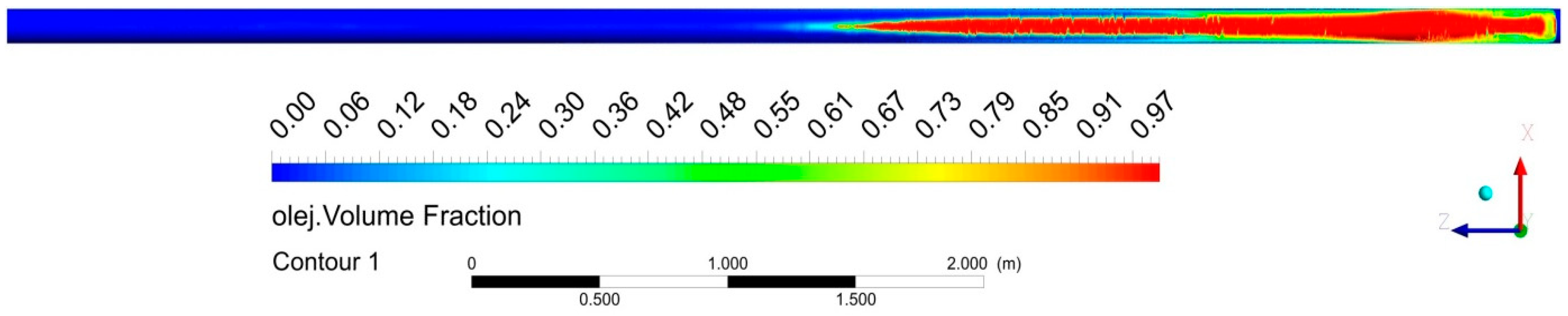
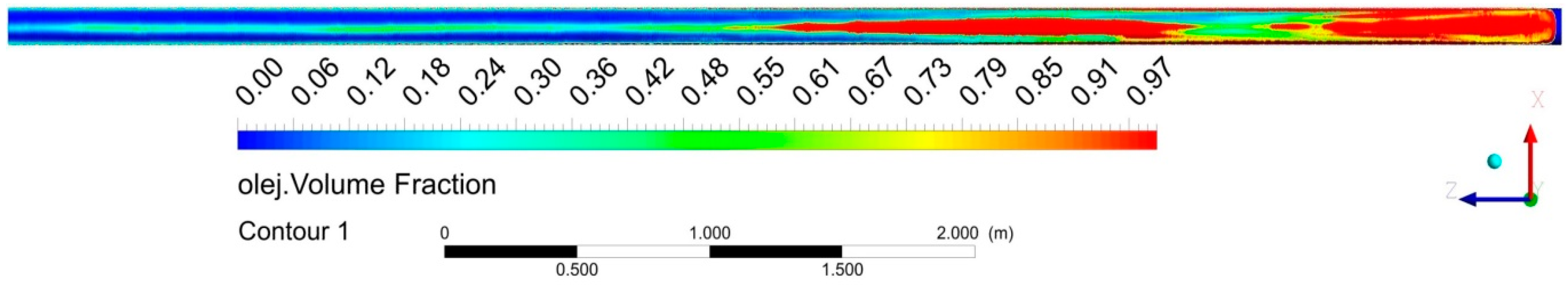
Three simulations were performed at 5, 5.5 and 7 m/s for a 25 mm pipe diameter.
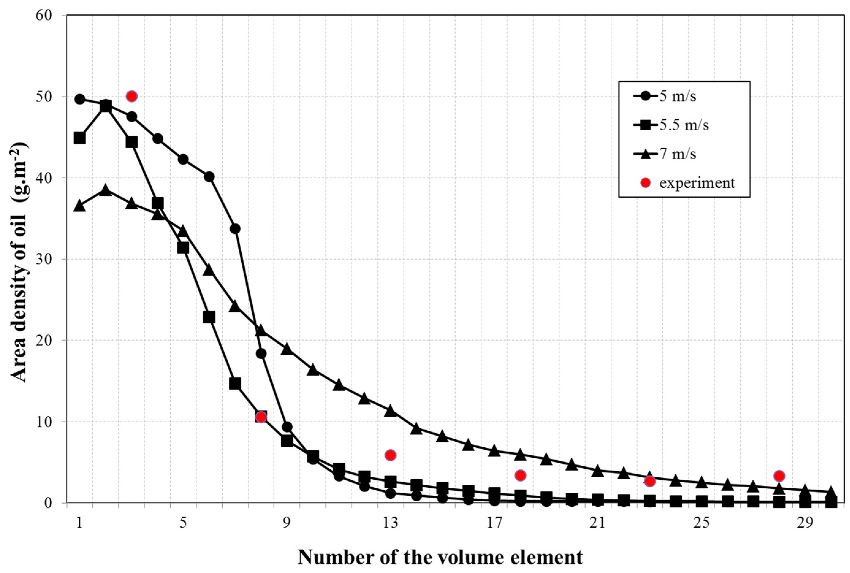
Figure 5 shows a plot of oil bulk density at three different speeds together with the measured data for a pipe diameter of 25 mm.
The more even distribution of the oil film was evident only at a speed above 5.5 m/s with a pipe diameter of 25 mm. Comparable results between the numerical calculation and the experiment could only be seen at the speed of 7 m/s.
Figure 6 and
Figure 7 show oil volume distribution at an air flow rate of 5.5 and 7 m/s respectively.
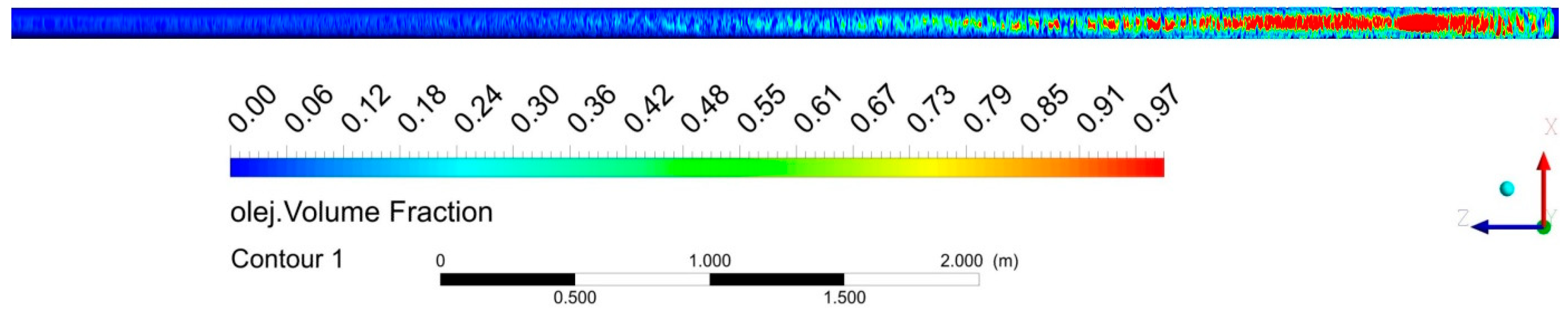
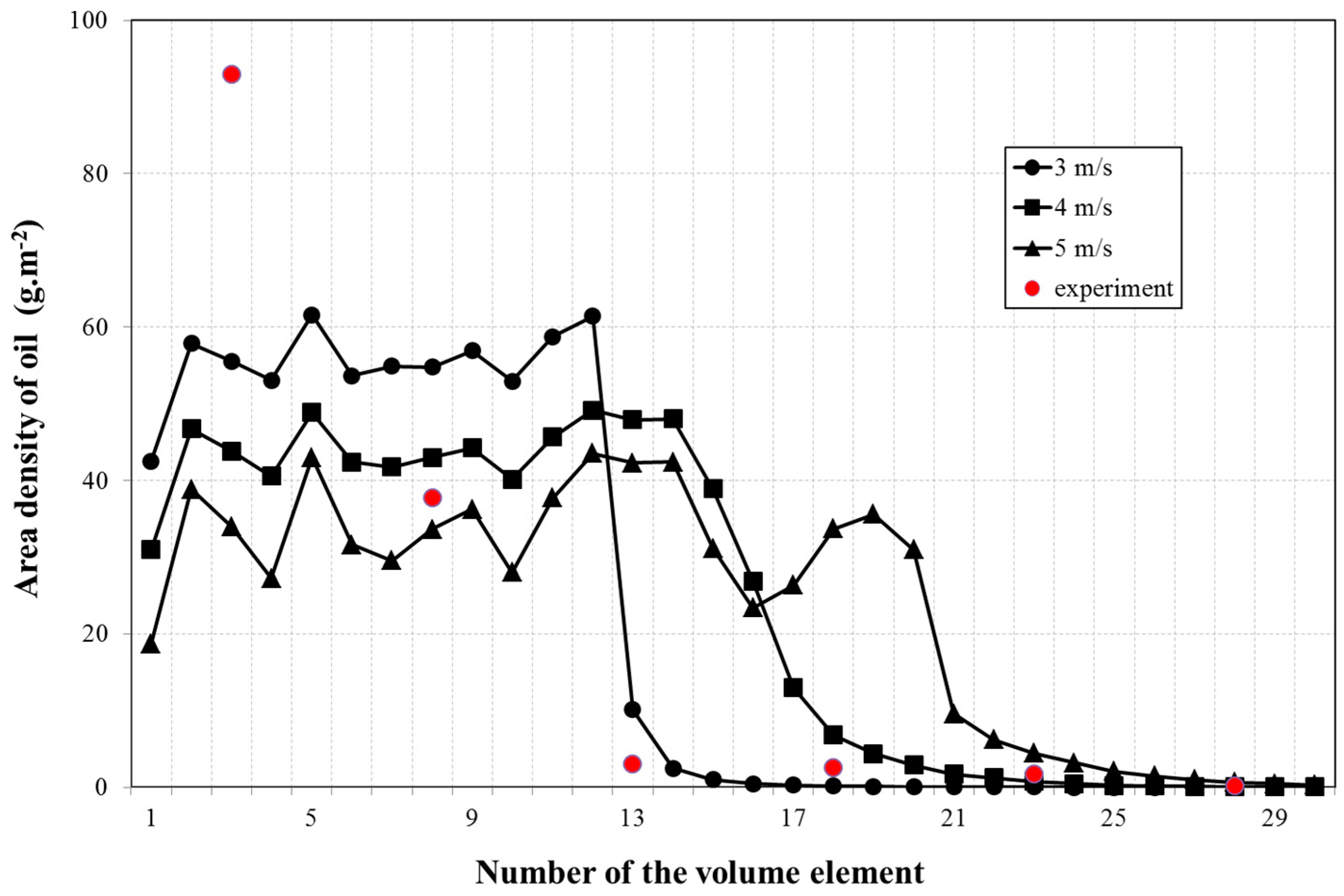
Figure 8 shows the areal density of oil at the speed of 3, 4 and 5 m/s passing through a 15 mm diameter pipeline according to experimental data. Due to the small diameter of the pipe, the distribution of oil in the first half of the pipe length is quite even according to numerical calculation.
At a pipe diameter of 15 mm, there is a match between the experiment and the numerical calculation at the lowest level, but the tendency of a sharp drop in oil density with increasing distance from the start of the pipe is still maintained. From the numerical calculation, it is also possible to adopt recommendation to maintain speed above 5 m/s.
Figure 9 shows oil volume distribution on the surface of the tube with a diameter of 15 mm at a speed of 5 m/s.
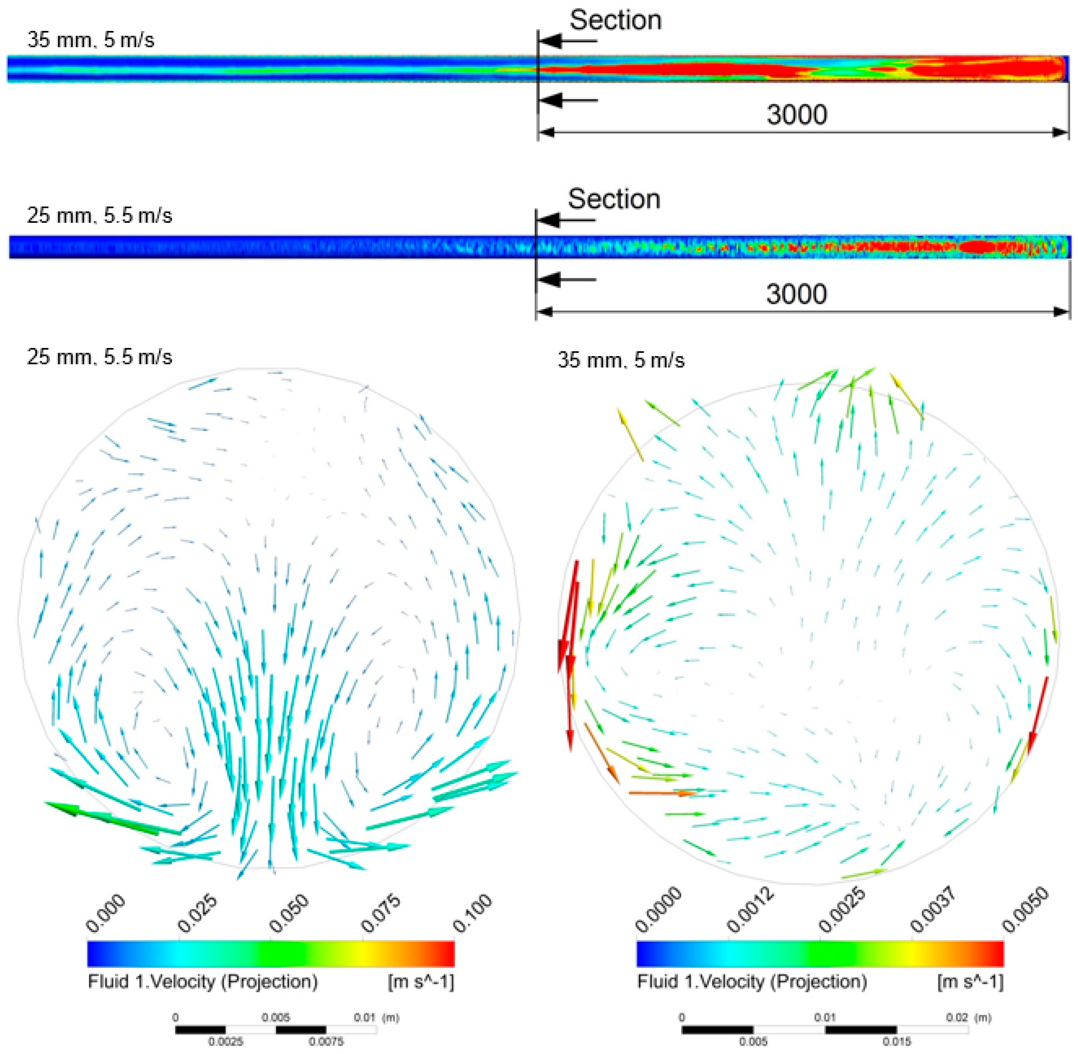
The considerable unevenness of the distribution of the areal density of the oil film over the length of the pipe between the individual pipe diameters is particularly noticeable in diameters of 15 and 35 mm. From the results of the numerical calculations, it is clear that the velocities of the fluid medium equal to or more precisely are less than 5 m/s and the course is significantly different from that of areal density as is achieved with a pipe diameter of 25 mm and higher speeds. This is due to the formation of two counter-rotating vortices, which are formed at speeds exceeding 5 m/s, causing the mixture to swirl and smooth the oil distribution over the length of the pipe surface.
Figure 10 shows a projection of a vector field in a plane perpendicular to the pipe at a distance of 3 m from the pipe inlet. On the left, there is a 25 mm diameter pipe at a speed of 5.5 m/s with counter-vortices displayed. On the right side, a pipe with diameter of 35 mm is displayed at a speed of 5 m/s without vortices, causing an uneven distribution of the oil fraction. By comparing the flow rate components of the flowing fluid in the displayed plane, it is evident that for low speeds, these components are negligible compared to the components at higher speeds.
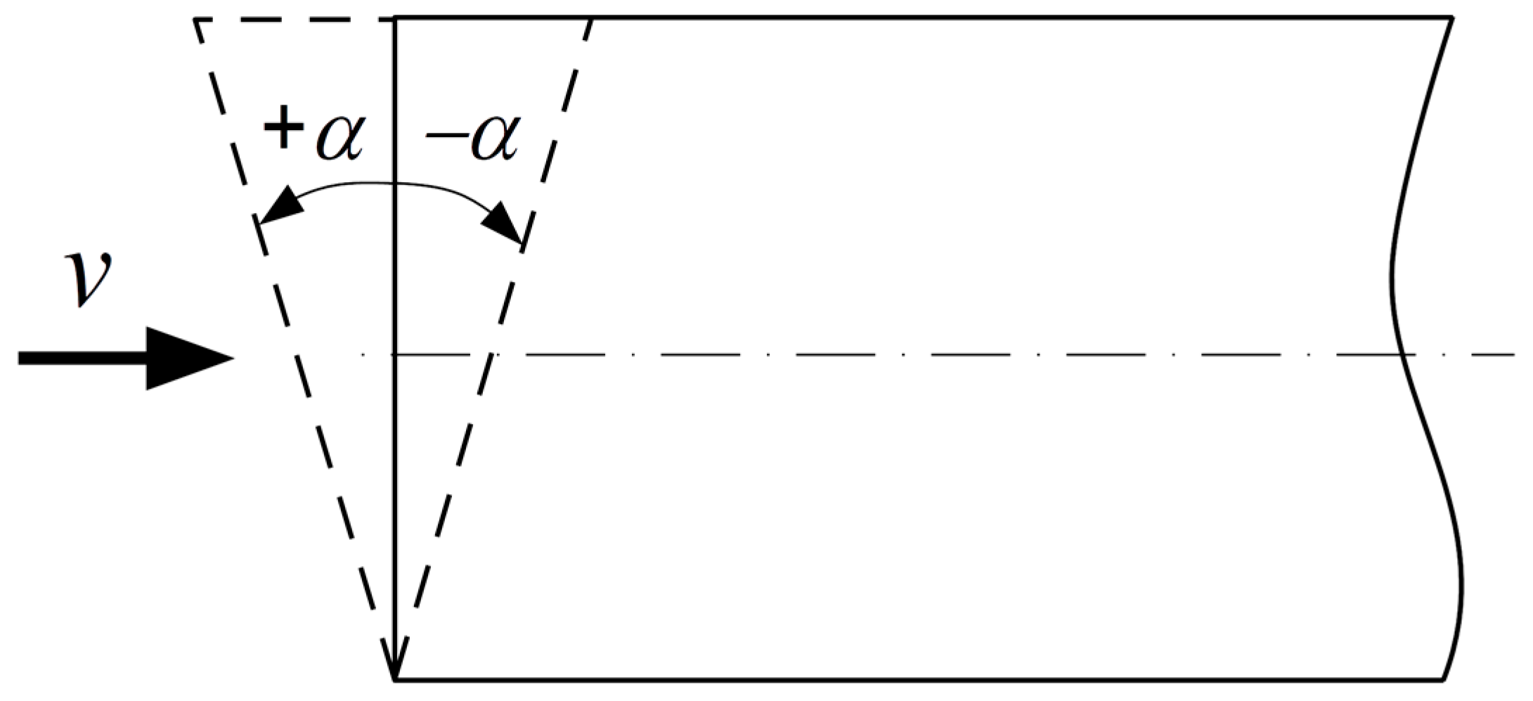
A sensitivity analysis was performed in order to evaluate the influence of the inaccuracy of the inlet angle of the multiphase mixture from the pipe axis. In its design, the results were taken for a pipe with an inner diameter of 25 mm with the corresponding inlet velocity of 5.5 m·s
−1. As shown in
Figure 11, the direction vector of the input rate was changed in the vertical position between values of +10 and −10° with a step 5°.
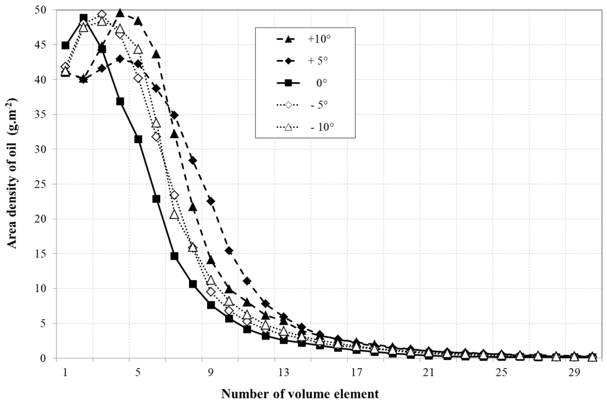
Figure 12 shows the results of the distribution of the areal density of the oil in the individual elements of the pipe depending on the angle of the input speed vector. A more pronounced deviation of the numerically calculated orientation angle occurs mainly with a positive orientation angle, at which a higher areal density of the oil is achieved due to a change in the trajectory of the fall of the oil particles.
Local deviations of areal density in individual sections of the pipe, when the inlet angle varies between −10 and +10°, obtain a value of 19 g·m−2. However, the basic shape of the orientation angle remains preserved and the minimum required surface density of the oil at an oil level of 1.4 g/m2, it is necessary to apply a sequential two-sided injection of the oil dispersion. The sensitivity to a small change in the angle of rise is therefore irrelevant.
3. Experimental Testing of Coating by Oil Dispersion
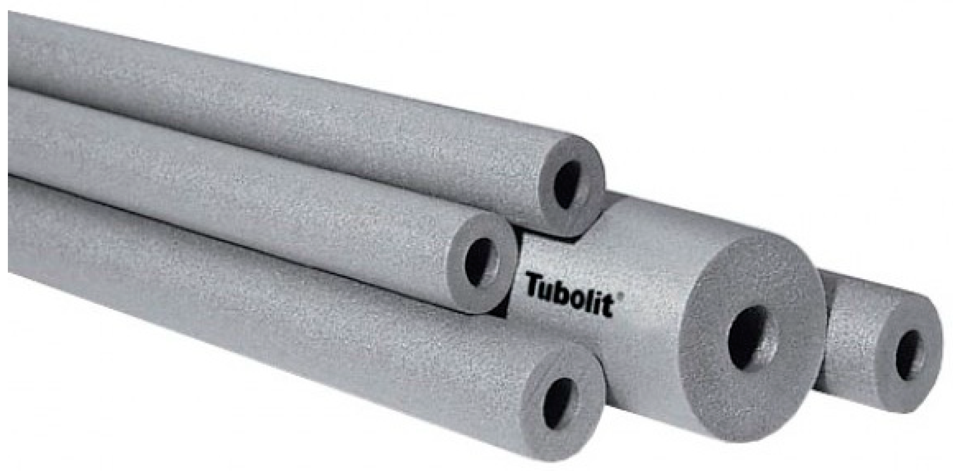
The solution parameters were based on 6 m long steel pipe coating requirements. Compared to the investigation of the technological feasibility of the problem, selected pipes with a d = 15, 25 and 35 mm diameter were chosen. Wall thickness in the case of modal analysis, mathematical modeling and experiments did not play any role in our findings. The material of the test and experimentally verified tubes was selected from polyethylene (PE) foam, available under the trade name “Mirelon” (
Figure 13), originally intended for insulation of water pipes for hot and cold water. This material was chosen for its consistency in mass across the entire cross section, for easier handling, price, and for the possibility of mechanical examination of the inner surface by touching it with a normal knife.
Adhesiveness of oil particles to the PE pipeline during the flow of the multiphase compound was numerically dealt with by application of the Antal et al. [
21] model, considering the wall lubrication coefficient (formula 4), whereas the results of numerical calculation of the application of the values Cw1 = −0.01 and Cw2 = 0.05 showed good match with the experiment results. The oil adhesiveness itself showed no dependence on the type of the pipe material.
The standard deviation of the weight of one meter of dry Mirelon with a 15 mm inner diameter is 0.082 g, the standard deviation for 25 mm is 0.18 g, and the standard deviation for 35 mm is 0.63 g. If steel pipes were to be used, it would have been very difficult to measure the oil layer inside the steel pipe as the certified scales with the required carrying capacity are not sufficiently precise and sensitive. The ratio between the weight of the pipe and the weight of the oil film is far more favorable for weighing a material such as “Mirelon”. For example, the dry weight of a 1 m long Mirelon tube with a 25 mm width and a wall thickness of 5 mm weighs approximately 11.5 g, the weight of a steel tube (EN 10 210-2 standard) of 25.3 mm diameter and a wall thickness of 0.8 mm (thinner is not normally produced) weighs approximately 515 g. The dry tube was weighed first, followed by weighing when wet. In percentage points, the differences thus obtained, i.e., between the dry and the wet tube, would have been too small. The measurement of the oil film itself would not have been possible.
Precise experimental measurements are given in previous works by Svetlík [
23,
24]. The chemical substance called “Anticorrid DFV 2001” is accurately described in detail in the manufacturer’s document described by Fuchs [
16]. Selected essential oil parameters of “Anticorrid DFV 2001” used in the experimental measurement are listed on the product card:
- -
vapor pressure: 1 mbar, at the temperature of 20 °C;
- -
density: 830 kg/m3, at the temperature of 25 °C, in compliance with DIN 51 757 standard;
- -
kinematic viscosity: 4.6 mm2/s, at the temperature of 20 °C, in compliance with DIN 51 562 standard.
Material used for measurement (Mirelon 15—the inner diameter of the pipe was 15 mm):
- -
“Mirelon 15” with a length of 2 m—adhered by a sticky tape to a 6 m tight section;
- -
“Mirelon 25” with a length of 2 m—adhered by a sticky tape to a 6 m tight section;
- -
“Mirelon 35” with a length of 2 m—adhered by a sticky tape to a 6 m tight section.
The original Mirelon tubes are 2 m long. Prior to the application, three pieces were joined together into a single tube of 6 m. The connection was made using a high quality adhesive tape, so that oil leakage from the joint was not possible.
Devices used in experimental verification:
- -
Apollo 50 compressor (air receiver 50 L, output power 1.5 kW, supplied air volume 158 L/m) with pressure regulator
- -
SMC LMV210-35 oil mist applicator;
- -
hand valve with a 10 mm hose in width and 5 m in length;
- -
calibrated scales with a certificate from the manufacturer A&D, TSQ 128/95-133 model, d: 0.01 g, e: 0.02 g, carrying capacity: 200 g.
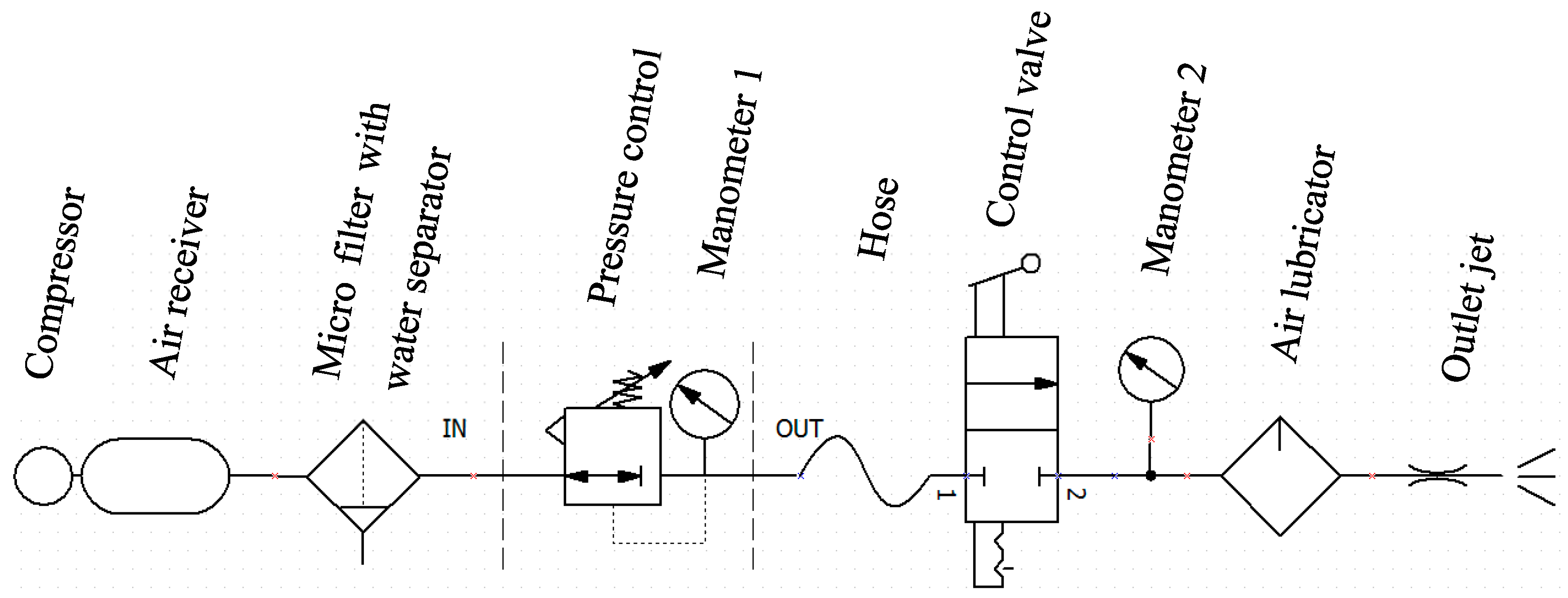
The experiment was realized on 30 December 2016. The temperature in the laboratory reached a constant value of 10 °C. The maximum working pressure was set at 8 bar during experimental measurement. The working pressure during the application of the oil dispersion with the open hand valve dropped to a constant value of 6 bar. A simplified circuit diagram of the pneumatic experimental measurement device is shown in
Figure 14.
In the experimental measurement, an oil dispersion was applied over the entire 6 m sections, which were cut into precise sections with a length of 1 m. These sections were then weighed on a calibrated scale and the results were accurately recorded.
The precise measuring procedure was as follows:
The compressor working pressure was set at 8 bar.
The compressor was switched on for a limited period of time (approximately 5 min.) to compress a 50 L of air tank until the compressor motor was automatically shut off.
The application nozzle was directed to the free space and the manual valve of the application nozzle was activated for about 4 s due to the oil intake into the lubrication feed pipe and for filling the lubricant itself.
The oil application nozzle was placed in high precision in front of the coated tube in a short time.
The manual valve, and the timer were activated simultaneously, and oil dispersion flowed into the tube.
After 15 s of application, the manual valve was deactivated and the oil dispersion stopped flowing into the tube.
The tube to which the oil fraction was applied was cut into 1 m long sections.
These 1 m sections were weighed on the precision scale.
The measured values were incorporated into the measurement protocol. The measurement results are shown in
Table 1,
Table 2 and
Table 3.
3.1. Conditions of Experimental Measurements
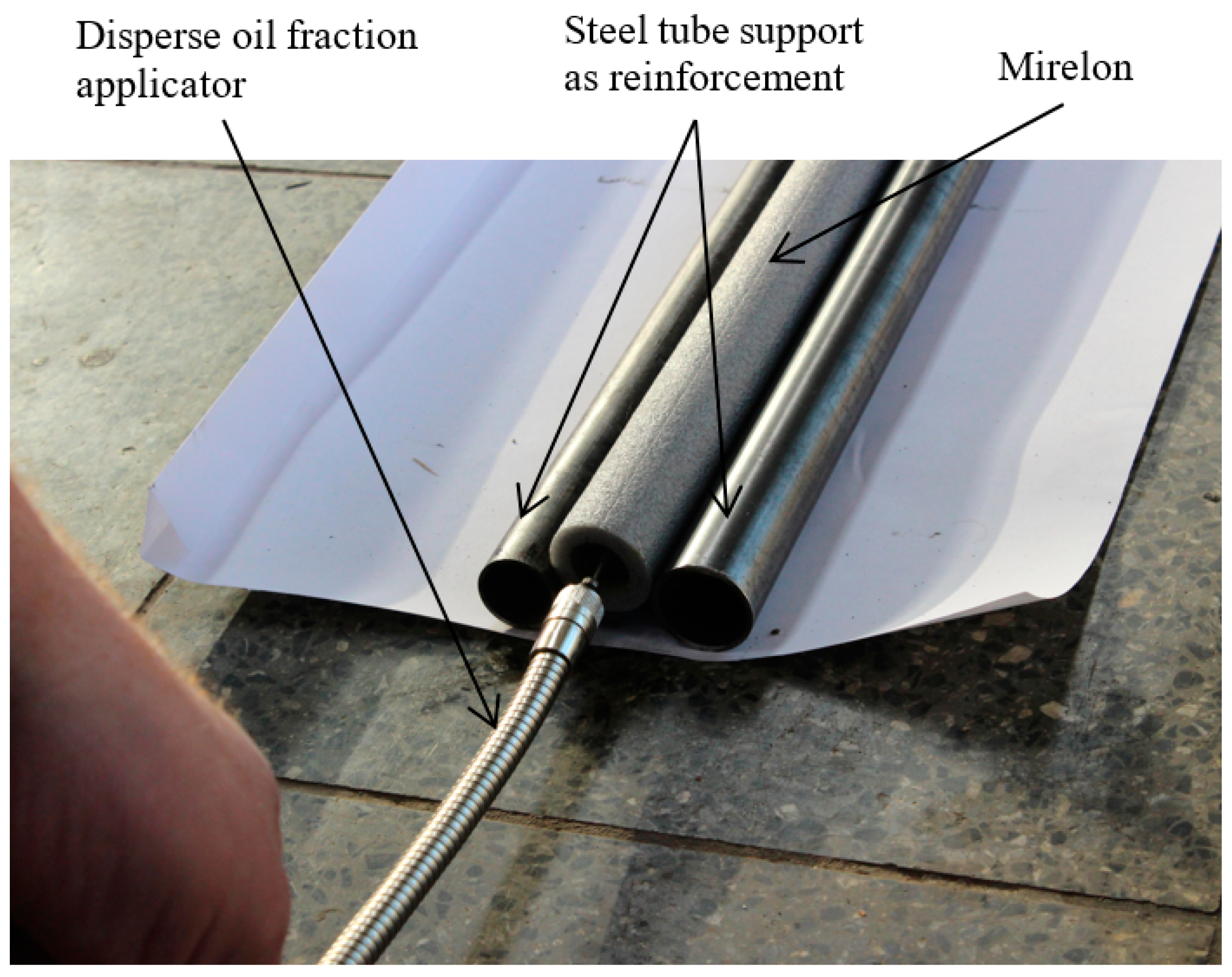
Measurements have been made with precision, with the utmost effort to maintain identical conditions. The ambient temperature did not change, the pressure of the air in the pressure vessel was always the same before each measurement, and the time of duration of each period was kept as precisely as possible. Application tubes, which served as a substitute for steel pipes to be treated with anticorrosive protection, were yielding and did not retain their shape. This phenomenon was eliminated by their stiffening with solid steel tubes, as seen in
Figure 15.
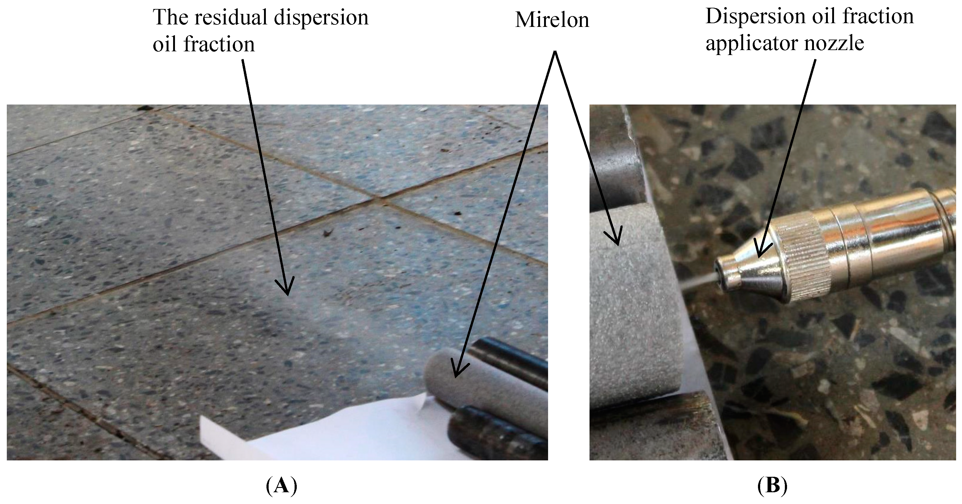
One important detail was also the detail of the position of the nozzle when entering the test tube. The output nozzle position was very important, as seen in
Figure 16B. It was necessary to keep its position in the pipe axis and also the application angle had to correspond to the axis of the pipe. Otherwise, if the nozzle or pipe nozzle is incorrect, it is likely that a larger amount of oil will settle in the initial part of the tube and consequently less oil will settle in the back as the oil mist will be less dense and will contain a weaker concentration of oil particles than it might have when the nozzle is correctly positioned.
In view of the texture of the dispersion oil fraction itself, it was important to run the applicator for a few seconds without the application tube just before application for a few seconds at the beginning, until the applicator mixing valve filled with applied oil from the container, thereby displacing the air bubbles that were in the application set. These bubbles were formed by gravity in intervals between applications themselves. Another, no less important detail in the application of the dispersion oil fraction in the tube is its outlet part, i.e., the exhaust. It is important for the exhaust not to be covered; its free outlet should be unimpeded, as seen in
Figure 16A. It is possible that further research will be able to propose a better aerodynamic element necessary to achieve the desired flow characteristic of the pipe outlet. From the point of view of measuring and observing identical conditions of measurement of tubes of different height clearance, it is appropriate to set identical conditions for the outlet of the pipe mouth.
3.2. Results of Experimental Measurements
Measurement of the coating of a slender pipe made of “Mirelon 15” (inner tube diameter is 15 mm) with oil dispersion fraction was performed with a calibrated A & D scale, the parameters of which are given above. In total, four sets of weights were measured by weighing the weight of the tubes, weighing six sectors of 1 m long “Mirelon 15” and six sectors of 1 m long “Mirelon 15” wet tubes after application of the oil fraction dispersion with identical parameters. The result of the first measurement set is shown in
Table 1.
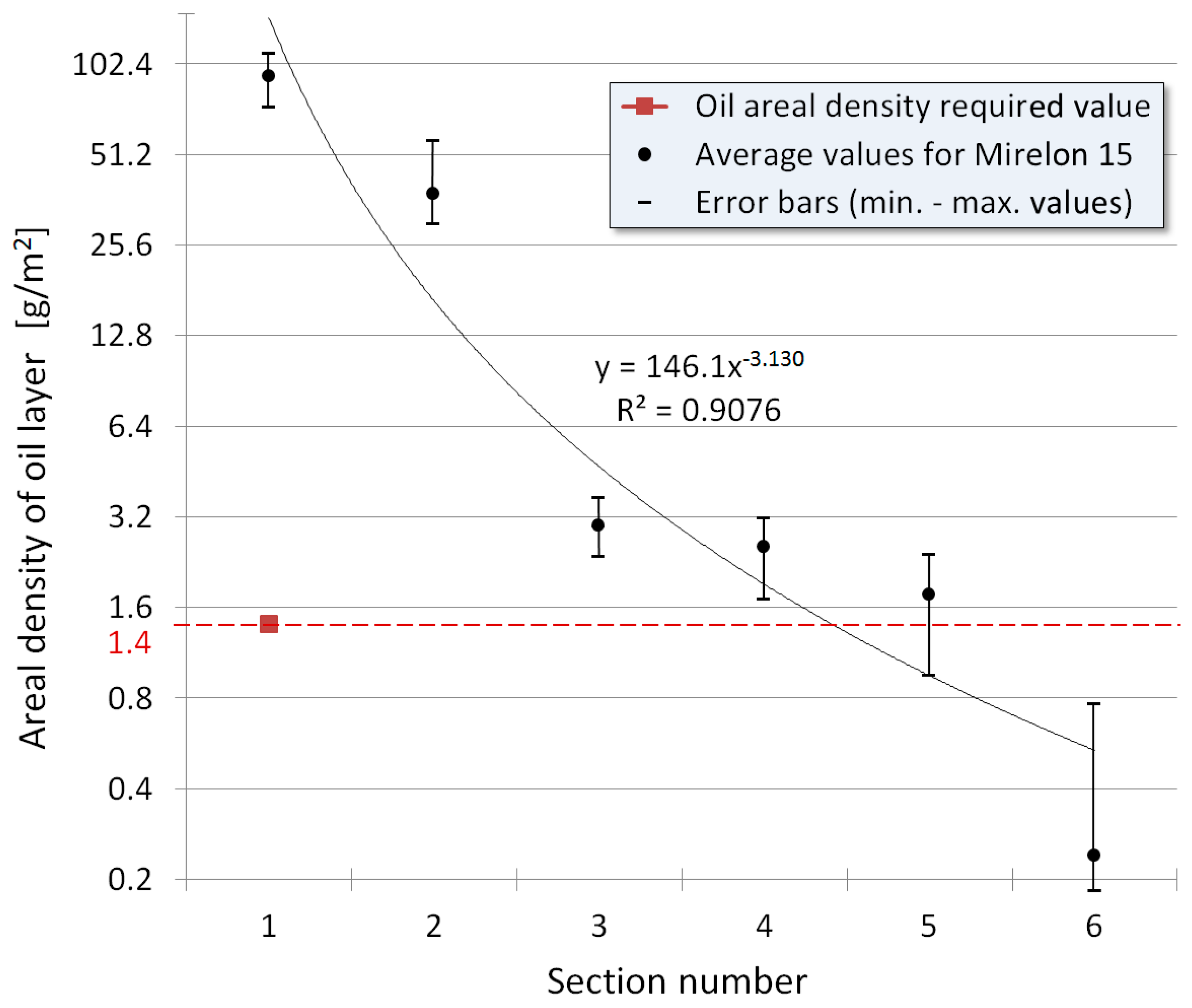
Figure 17 shows the results of the first set of measurements with data taken from
Table 2. The oil filler limit value for guaranteed anti-corrosion protection according to the oil product card is 1.4 g/m
2. It follows that under the given conditions and with a pipe with the geometrical parameters of the “Mirelon 15” pipe, the sufficient oil film layer extends approximately to 4.6 m. However, it should be kept in mind that the inner surface of the pipe is not evenly coated with the oil film. The biggest differences will be between the highest and lowest points of the inner cross-section of the coated pipe. It can be said, therefore, that the method under the given conditions is not suitable for anticorrosive protection at the originally required length of 6 m.
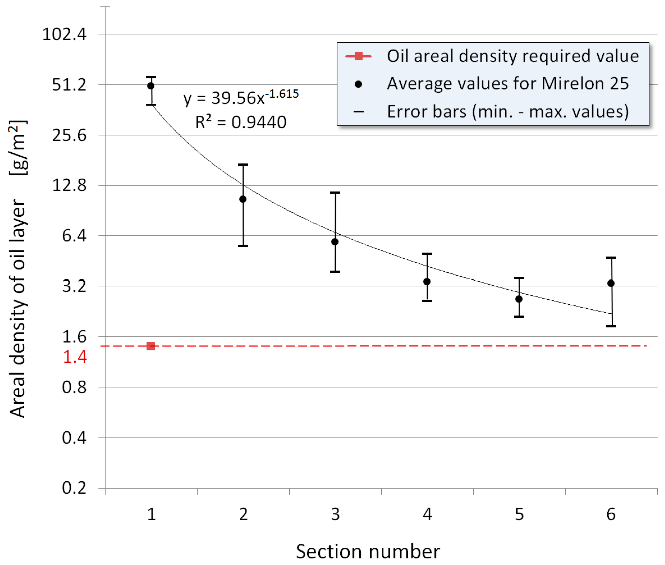
Figure 18 shows the results from the second set of measurements with data taken from
Table 3. The limit value of enough oil film is identical to the first set of measurements, i.e., 1.4 g/m
2.
Figure 4 shows that, under the given conditions and with the pipe geometrical parameters of the “Mirelon 25” pipe, sufficient oil film layer extends approximately to the required distance of 6 m. Thus, it appears that the greater fluorescence of the pipe is more suitable for the application of an anti-corrosion protection at the given oil dispersion application parameters.
However, it should be remarked that these are only average values with unequal distribution of the thickness of the applied oil layer on the inner surface of the pipe. It is probable that at the top of the cross section, the anti-corrosion protection layer will still be inadequate.
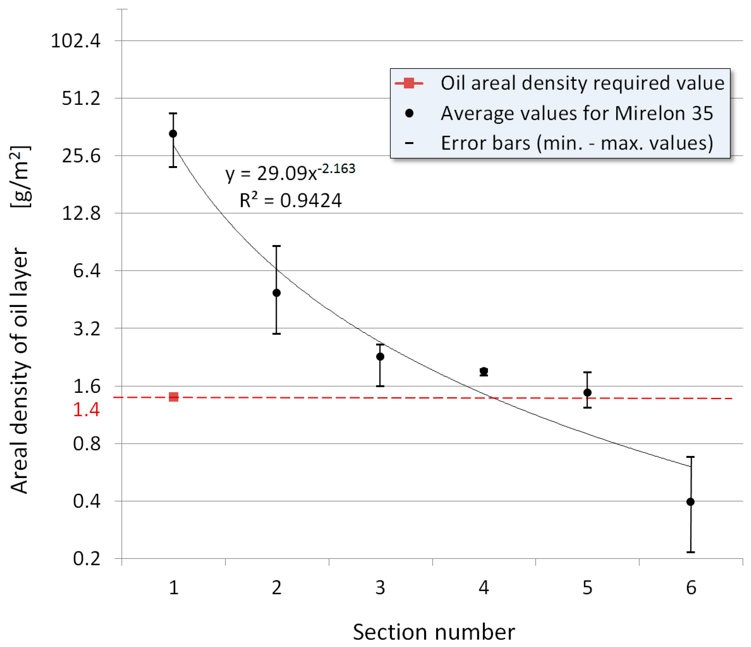
Figure 19 shows the results of the third set of measurements with data taken from
Table 3. The limit value of the oil film sufficient for anticorrosive protection according to the oil product card is 1.4 g/m
2. It follows that under the given conditions and with a tube with the geometrical parameters of the “Mirelon 35”, a sufficient oil film layer extends to approximately 4 m. As in the previous cases, the inner surface of the pipe is not evenly coated with the oil film. The biggest differences will be between the highest and lowest points of the inner cross-section of the coated pipe. It can be said, therefore, that the method under the given conditions is not suitable for anticorrosive protection at the originally required length of 6 m.
4. Discussion
We believe that its useful to approximate the results measured by the experiment and try to find and algorithmize the relationship between variables such as: height clearance of the pipe, pipe length, flow rate of the dispersed oil fraction, and dynamic viscosity of the applied substance.
Achieving the anti-corrosion protection of inaccessible slim spots is not a simple matter. The tightness of the pipe makes the transport of the microparticle of the applied substance (in our case, the Anticorrid DFV 2001 oil) to the lateral distance complicated. Most often, heavier or larger particles are caught at the beginning of the pipe. Furthermore, only medium and large particles with a lower potential for attaching to the inner surface of the pipe continue further. It is therefore advisable to know the distance, depending on the height clearance of the pipe, in which the particles of the dispersion oil fraction are in sufficient quantity to reach the required limit value prescribed by the manufacturer as 1.4 g/m2.
In assessing the technical reliability of the device described above (
Figure 14) and its application success, it is appropriate to apply some diagnostic tools used to diagnose oil condition in machinery as described by Baron [
25].
5. Conclusions
By appropriately selecting numerical simulation settings, it is possible to achieve a relatively good match between the measured and numerically calculated values of the areal density of the oil film deposited on the inner surface of the pipe. The basic problem of using numerical solutions is the considerable dependence of oil deposition over the length of the pipe from a large number of selected parameters. It is essential to correctly select the input speed, the roughness of the pipe and the resistance coefficients. Due to the fact that numerical calculation dealt with the flow of viscous fluid with oil particles, simultaneously taking into account turbulent flow, the pipe resistance is also accounted for in the calculation. However, the paper did not deal with pressure drops due to their irrelevance with respect to the resulting oil fraction layer on the pipe’s surface. There is substantial adherence to the speed at the entrance into the pipe and the oil volume fraction (compliance with the margin conditions). The pipe’s resistance to the flow of the fluid was causing a pressure drop ranging between 75 and 138 Pa subject to the pipe’s diameter (at 5 m∙s−1).
The deviation of the angle between the pipe axis and the speed at the inlet to the pipe during oil mist injection does not have a significant effect on the distribution of the areal density of the oil film due to the rapid stabilization of the current.
As can be seen from
Figure 2,
Figure 5 and
Figure 8, simulation and experimental measurement results are not always accurate. It is due to the imperfection of measurement and simulation. Despite the fact that a strong emphasis was placed on the best possible simulation, as can be seen in
Figure 1, as the cross-linking of the elements with respect to the most serious object where the trapped oil micro particles are made, there is still a large amount of input variables into the simulation software. The simulations themselves were performed on a high-performance computer with 36 processor cores, one simulation lasting over 24 h. However, it can be said that the results of simulation, despite its imperfection, can be considered to be the same as experimental measurements, which we consider to be the starting point for further reflections on the investigated issue.
Experimental measurement also involved a number of influential factors that had to be unified within the individual metering occurrences and eliminated as much as possible.
The resulting graphs of the dispersion oil fraction plot for the different pipe diameters can be taken as the primary information for possible real use in practice. In general, it can be said a few important findings have been made and recommendations should be respected:
- −
The pipes during the application of the dispersion oil fraction should be rotated to achieve a uniform distribution of the oil layer along their inner surface.
- −
The entry of the dispersion oil fraction through the nozzle must be as accurate as possible, aligned with the pipe axis, and the angle between the axis of the pipe and the nozzle axis should be the same.
- −
Ensure the texture of the dispersed oil fraction without dirt and air bubbles is consistent.
- −
Ensure the ambient parameters, such as: temperature, flow rate of the dispersion oil fraction, air pressure in the compressor reservoir are stable, ensure that the opening for the dispersed oil fraction to escape the treated pipe is open.
After observing the above parameters, the method can be used to coat steel (or other materials) pipes and thereby obtain the desired anticorrosive protection of the inner surface of slim pipes.


