Competitive Influence Maximization within Time and Budget Constraints in Online Social Networks: An Algorithmic Approach

Abstract
1. Introduction
- We formulate Time constraint Competitive Linear Threshold () model by extending Competitive Linear Threshold model in [21,22] to simulate competitive influence within time constraint . Given two competitors A and B who need to advertise their productions on OSNs, assume that we know nodes that are activated by B (B-seed set). Given the limited budget L, heterogeneous cost of each node to active by A (i.e., each node has a cost to add it into A-seed set), and the time constraint , we study problem, which aims to seek A-seed set nodes within limited budget L and time constraint to maximize nodes influenced by A under model. We then show that is NP-hard and the objective function is neither submodular nor supermodular.
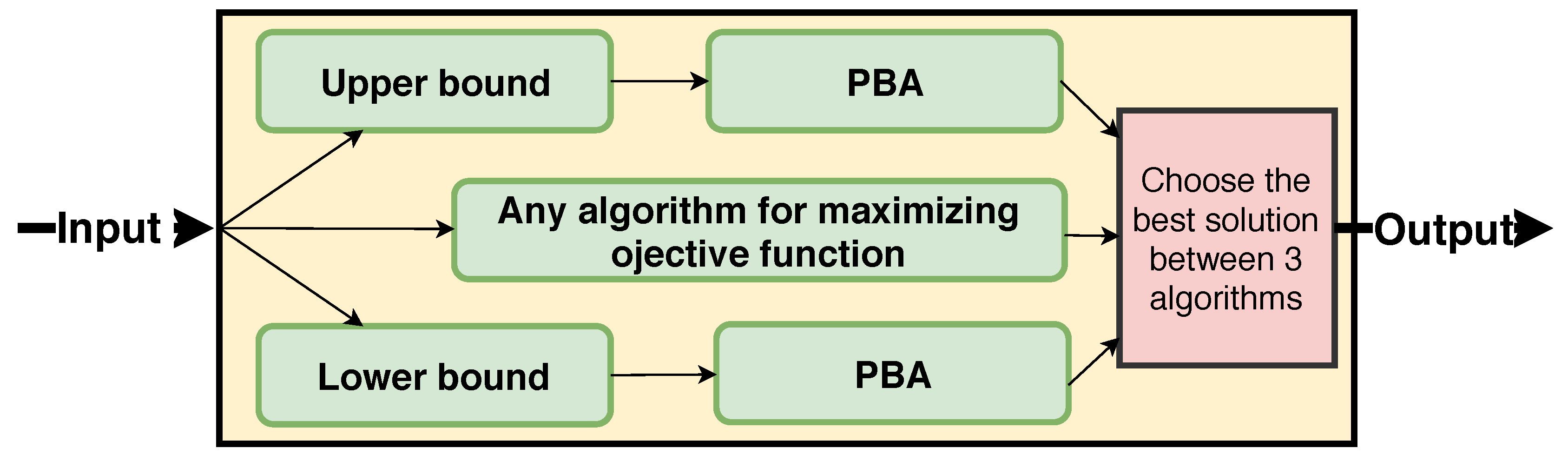
- We propose , an efficient randomized algorithm based on Sandwich approximation and polling method. We first design upper bound and lower bound submodular functions of the objective function and develop a polling-based approximation algorithm to find the solution of bound functions that guarantees approximation ratio of with high probability. Based on that, the Sandwich framework approximation in [16] is applied to give a data-dependent approximation factor.
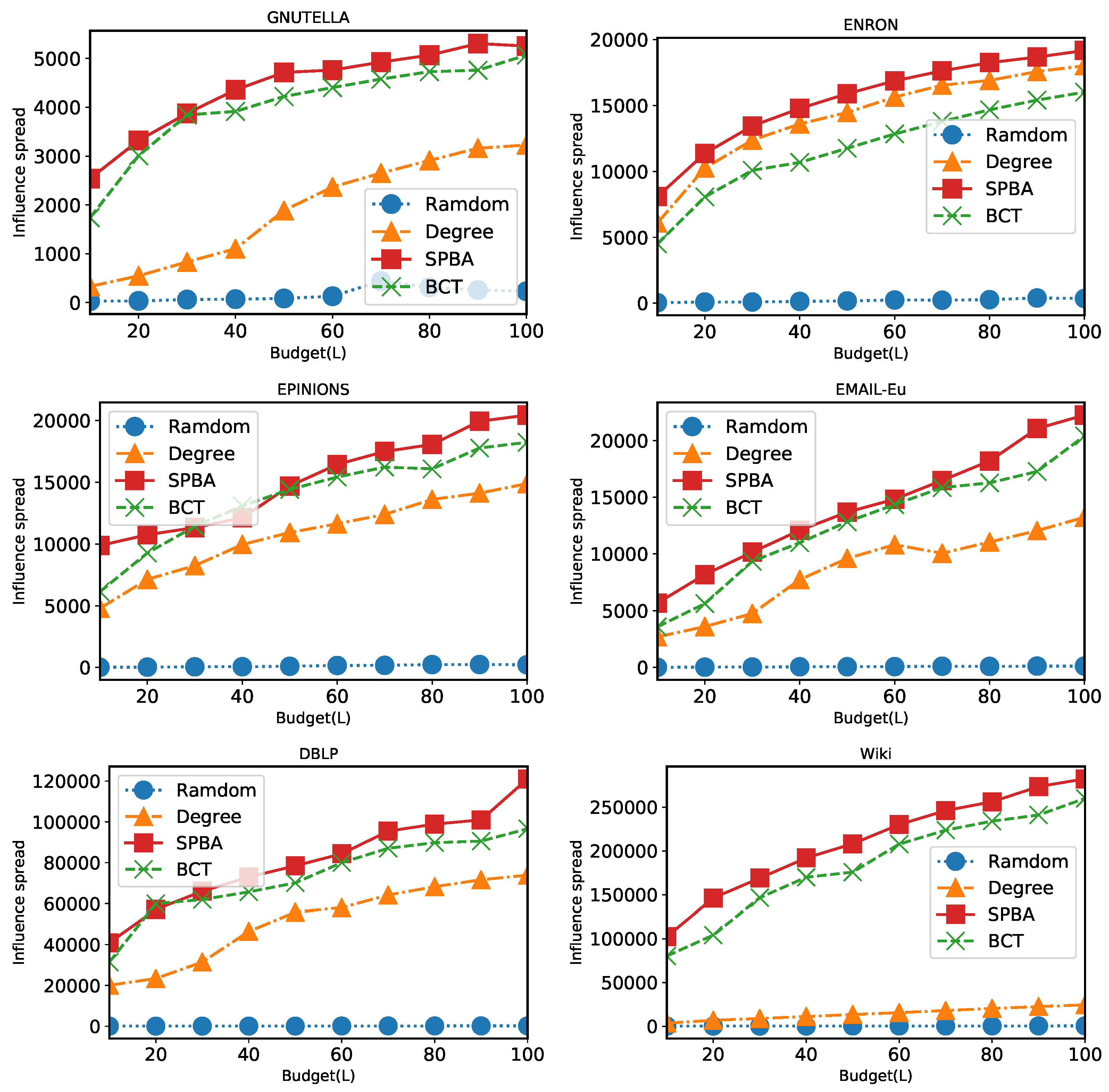
- We conducted extensive experiments on various real social networks. The experiments suggest that provides significantly higher quality solutions than existing methods including baseline algorithms and influence maximization algorithms. Furthermore, we also demonstrate that our algorithm can scale to million-scale networks within about 1.5 min.
2. Related Work
2.1. Influence Maximization
2.2. Competitive Influence Maximization
3. Preliminaries
3.1. Competitive Linear Threshold () Model
- At step , .
- At step , it first sets and . Each node becomes A-active ifNode v becomes B-active ifin the case when node u that has the total influence weight of two competitors are greater than corresponding thresholds. Chen et al. [21] summarized tie-breaking rules can be used to determine whether v is A-active or B-active.
- –
- Fixed probability tie-breaking rule (TB-FP): TB-FP means that with a fixed probability p, u becomes A-active with probability p and becomes B-active with probability . The special cases of this rule include TB-FP(A)-competitor A’s dominance, TB-FP(B)-competitor B’s dominance.
- –
- Proportional Probability tie-breaking rule (TB-PP): is A-active successful attempt set of u and is B-active successful attempt set of u. Node v becomes A-active with probability , and u is B-activated with probability .
- Once a node becomes activated (A-active or B-active), its status remains in next steps. The propagation process ends when no more nodes can be activated.
3.2. Competitive Influence Maximization
4. Models and Problem Definition
4.1. Time Constraint Competitive Linear Threshold () Model
- At step , .
- At step , first set and . Each node becomes A-active ifNode v becomes B-active if
- If in step t, a node v hasWe propose weight proportional probability tie-breaking rule (TB-WPP) to determine its state. Accordingly, v is A-activated with probability.and v is B-activated with probability
- Once a node becomes activated (A-active or B-active), it keeps this status in the next steps. The propagation process ends after hops of propagation or no more nodes can be activated.
4.2. Budgeted Competitive Influence Maximization Problem
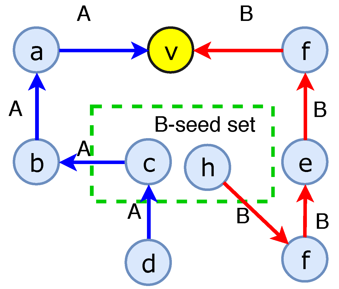
4.3. Competitive Live-Edge () Model
- At step , and .
- At step , first set and . A node becomes A-active if v is reachable from in one step in (i.e., ) but not reachable from in one step in (i.e., ), then v is in . Symmetrically, if v is reachable from in one step in but not reachable from in one step in , then v is in .
- If at step , v is reachable from in one step in and reachable from in one step in , v is A-activated with probabilityand v is B-activated with probability
- The process of propagation ends after hop or no more nodes can be activated.
5. Our Proposed Algorithm for Problem
5.1. Lower and Upper Bound Functions
5.1.1. Upper Bound Function
| Algorithm 1: Generate set. |
 |
5.1.2. Lower Bound Submodular Function
| Algorithm 2: Check the distance from u to B on —. |
 |
5.2. Polling-Based Algorithm for Maximum Bound Functions
| Algorithm 3: Polling-Based Approximation algorithm (). |
 |
| Algorithm 4: Generate set. |
 |
5.2.1. Description of
| Algorithm 5: Greedy algorithm for Budgeted Maximum Coverage problem—. |
 |
| Algorithm 6: Check quality of solution (). |
 |
5.2.2. Theoretical Analysis
5.2.3. Improved Guarantees with Tightened Bound
5.3. Sandwich Approximation
| Algorithm 7: Sandwich Approximation base on algorithm (). |
| Input: Graph , budget , and Output: Seed set 1. 2. 3. a solution for maximizing by any algorithm. 4. 5. return S; |
6. Experiments
6.1. Experimental Settings
6.1.1. Datasets
6.1.2. Algorithm Compared
- : An influence maximization algorithm under the heterogeneous selecting cost. The reason we chose to compare is that is a variant of and considers of nodes with arbitrary costs.
- : This algorithm selects nodes with the highest degree and we keep on adding the highest-degree nodes until total costs of the selection of nodes exceeds L.
- : This algorithm randomly selects nodes within budget L.
6.1.3. Parameters
6.2. Results
6.2.1. Comparison of Algorithms under General Case
6.2.2. Comparison of Algorithms under Unit-Cost Setting
6.2.3. Comparison of Running Time
6.2.4. Impact of
7. Conclusions
Author Contributions
Funding
Conflicts of Interest
Appendix A
References
- Kempe, D.; Kleinberg, J.M.; Tardos, É. Maximizing the spread of influence through a social network. In Proceedings of the Ninth ACM SIGKDD International Conference on Knowledge Discovery and Data Mining, Washington, DC, USA, 24–27 August 2003; pp. 137–146. [Google Scholar] [CrossRef]
- Borgs, C.; Brautbar, M.; Chayes, J.T.; Lucier, B. Maximizing Social Influence in Nearly Optimal Time. In Proceedings of the Twenty-Fifth Annual ACM-SIAM Symposium on Discrete Algorithms, SODA 2014, Portland, ON, USA, 5–7 January 2014; pp. 946–957. [Google Scholar] [CrossRef]
- Leskovec, J.; Krause, A.; Guestrin, C.; Faloutsos, C.; VanBriesen, J.M.; Glance, N.S. Cost-effective outbreak detection in networks. In Proceedings of the 13th ACM SIGKDD International Conference on Knowledge Discovery and Data Mining, San Jose, CA, USA, 12–15 August 2007; pp. 420–429. [Google Scholar] [CrossRef]
- Nguyen, H.T.; Thai, M.T.; Dinh, T.N. Stop-and-Stare: Optimal Sampling Algorithms for Viral Marketing in Billion-scale Networks. In Proceedings of the 2016 International Conference on Management of Data, SIGMOD Conference 2016, San Francisco, CA, USA, 26 June–1 July 2016; pp. 695–710. [Google Scholar] [CrossRef]
- Tang, Y.; Xiao, X.; Shi, Y. Influence maximization: Near-optimal time complexity meets practical efficiency. In Proceedings of the International Conference on Management of Data, SIGMOD 2014, Snowbird, UT, USA, 22–27 June 2014; pp. 75–86. [Google Scholar] [CrossRef]
- Tang, Y.; Shi, Y.; Xiao, X. Influence Maximization in Near-Linear Time: A Martingale Approach. In Proceedings of the 2015 ACM SIGMOD International Conference on Management of Data, Melbourne, Victoria, Australia, 31 May–4 June 2015; pp. 1539–1554. [Google Scholar] [CrossRef]
- Nguyen, H.T.; Thai, M.T.; Dinh, T.N. A Billion-Scale Approximation Algorithm for Maximizing Benefit in Viral Marketing. IEEE/ACM Trans. Netw. 2017, 25, 2419–2429. [Google Scholar] [CrossRef]
- Chen, W.; Yuan, Y.; Zhang, L. Scalable Influence Maximization in Social Networks under the Linear Threshold Model. In Proceedings of the 10th IEEE International Conference on Data Mining, Sydney, Australia, 14–17 December 2010; pp. 88–97. [Google Scholar] [CrossRef]
- Chen, W.; Wang, C.; Wang, Y. Scalable influence maximization for prevalent viral marketing in large-scale social networks. In Proceedings of the 16th ACM SIGKDD International Conference on Knowledge Discovery and Data Mining, Washington, DC, USA, 25–28 July 2010; pp. 1029–1038. [Google Scholar] [CrossRef]
- Nguyen, H.; Zheng, R. On Budgeted Influence Maximization in Social Networks. IEEE J. Sel. Areas Commun. 2013, 31, 1084–1094. [Google Scholar] [CrossRef]
- Bharathi, S.; Kempe, D.; Salek, M. Competitive Influence Maximization in Social Networks. In Proceedings of the Internet and Network Economics, Third International Workshop, WINE 2007, San Diego, CA, USA, 12–14 December 2007; pp. 306–311. [Google Scholar] [CrossRef]
- Lu, W.; Bonchi, F.; Goyal, A.; Lakshmanan, L.V.S. The bang for the buck: Fair competitive viral marketing from the host perspective. In Proceedings of the 19th ACM SIGKDD International Conference on Knowledge Discovery and Data Mining, KDD 2013, Chicago, IL, USA, 11–14 August 2013; pp. 928–936. [Google Scholar] [CrossRef]
- Chen, W.; Collins, A.; Cummings, R.; Ke, T.; Liu, Z.; Rincón, D.; Sun, X.; Wang, Y.; Wei, W.; Yuan, Y. Influence Maximization in Social Networks When Negative Opinions May Emerge and Propagate. In Proceedings of the Eleventh SIAM International Conference on Data Mining, SDM 2011, Mesa, AZ, USA, 28–30 April 2011; pp. 379–390. [Google Scholar] [CrossRef]
- Liu, W.; Yue, K.; Wu, H.; Li, J.; Liu, D.; Tang, D. Containment of competitive influence spread in social networks. Knowl.-Based Syst. 2016, 109, 266–275. [Google Scholar] [CrossRef]
- Bozorgi, A.; Samet, S.; Kwisthout, J.; Wareham, T. Community-based influence maximization in social networks under a competitive linear threshold model. Knowl.-Based Syst. 2017, 134, 149–158. [Google Scholar] [CrossRef]
- Lu, W.; Chen, W.; Lakshmanan, L.V.S. From Competition to Complementarity: Comparative Influence Diffusion and Maximization. PVLDB 2015, 9, 60–71. [Google Scholar] [CrossRef]
- Carnes, T.; Nagarajan, C.; Wild, S.; van Zuylen, A. Maximizing Influence in a Competitive Social Network: A Follower’s Perspective. In Proceedings of the Ninth International Conference on Electronic Commerce, Minneapolis, MN, USA, 19–22 August 2007; pp. 351–360. [Google Scholar]
- Wang, X.; Zhang, Y.; Zhang, W.; Lin, X. Dominated competitive influence maximization with time-critical and time-delayed diffusion in social networks. J. Comput. Sci. 2018, 28, 318–327. [Google Scholar] [CrossRef]
- Yan, R.; Zhu, Y.; Li, D.; Ye, Z. Minimum cost seed set for threshold influence problem under competitive models. World Wide Web 2018. [Google Scholar] [CrossRef]
- Khuller, S.; Moss, A.; Naor, J. The Budgeted Maximum Coverage Problem. Inf. Process. Lett. 1999, 70, 39–45. [Google Scholar] [CrossRef]
- Chen, W.; Lakshmanan, L.V.S.; Castillo, C. Information and Influence Propagation in Social Networks; Synthesis Lectures on Data Management, Morgan & Claypool Publishers: Williston, VT, USA, 2013. [Google Scholar]
- He, X.; Song, G.; Chen, W.; Jiang, Q. Influence Blocking Maximization in Social Networks under the Competitive Linear Threshold Model. In Proceedings of the Twelfth SIAM International Conference on Data Mining, Anaheim, CA, USA, 26–28 April 2012; pp. 463–474. [Google Scholar] [CrossRef]
- Valiant, L.G. The Complexity of Enumeration and Reliability Problems. SIAM J. Comput. 1979, 8, 410–421. [Google Scholar] [CrossRef]
- Borodin, A.; Filmus, Y.; Oren, J. Threshold Models for Competitive Influence in Social Networks. In Proceedings of the Internet and Network Economics—6th International Workshop, WINE 2010, Stanford, CA, USA, 13–17 December 2010; pp. 539–550. [Google Scholar] [CrossRef]
- Wang, X.; Zhang, Y.; Zhang, W.; Lin, X. Efficient Distance-Aware Influence Maximization in Geo-Social Networks. IEEE Trans. Knowl. Data Eng. 2017, 29, 599–612. [Google Scholar] [CrossRef]
- Song, C.; Hsu, W.; Lee, M. Targeted Influence Maximization in Social Networks. In Proceedings of the 25th ACM International Conference on Information and Knowledge Management, CIKM 2016, Indianapolis, IN, USA, 24–28 October 2016; pp. 1683–1692. [Google Scholar] [CrossRef]
- Li, Y.; Zhang, D.; Tan, K. Real-time Targeted Influence Maximization for Online Advertisements. PVLDB 2015, 8, 1070–1081. [Google Scholar] [CrossRef]
- Lin, Y.; Chen, W.; Lui, J.C.S. Boosting Information Spread: An Algorithmic Approach. In Proceedings of the 33rd IEEE International Conference on Data Engineering, ICDE 2017, San Diego, CA, USA, 19–22 April 2017; pp. 883–894. [Google Scholar] [CrossRef]
- Goyal, A.; Lu, W.; Lakshmanan, L.V.S. CELF++: Optimizing the greedy algorithm for influence maximization in social networks. In Proceedings of the 20th International Conference on World Wide Web, WWW 2011, Hyderabad, India, 28 March–1 April 2011; pp. 47–48. [Google Scholar] [CrossRef]
- Jung, K.; Heo, W.; Chen, W. IRIE: Scalable and Robust Influence Maximization in Social Networks. In Proceedings of the 12th IEEE International Conference on Data Mining, ICDM 2012, Brussels, Belgium, 10–13 December 2012; pp. 918–923. [Google Scholar] [CrossRef]
- Goyal, A.; Lu, W.; Lakshmanan, L.V.S. SIMPATH: An Efficient Algorithm for Influence Maximization under the Linear Threshold Model. In Proceedings of the 11th IEEE International Conference on Data Mining, ICDM 2011, Vancouver, BC, Canada, 11–14 December 2011; pp. 211–220. [Google Scholar] [CrossRef]
- Budak, C.; Agrawal, D.; El Abbadi, A. Limiting the spread of misinformation in social networks. In Proceedings of the 20th International Conference on World Wide Web, WWW 2011, Hyderabad, India, 28 March–1 April 2011; pp. 665–674. [Google Scholar] [CrossRef]
- Tong, G.A.; Wu, W.; Guo, L.; Li, D.; Liu, C.; Liu, B.; Du, D. An efficient randomized algorithm for rumor blocking in online social networks. In Proceedings of the 2017 IEEE Conference on Computer Communications, INFOCOM 2017, Atlanta, GA, USA, 1–4 May 2017; pp. 1–9. [Google Scholar] [CrossRef]
- Chung, F.R.K.; Lu, L. Survey: Concentration Inequalities and Martingale Inequalities: A Survey. Int. Math. 2006, 3, 79–127. [Google Scholar] [CrossRef]
- Dagum, P.; Karp, R.M.; Luby, M.; Ross, S.M. An Optimal Algorithm for Monte Carlo Estimation. SIAM J. Comput. 2000, 29, 1484–1496. [Google Scholar] [CrossRef]
- Leskovec, J.; Kleinberg, J.M.; Faloutsos, C. Graph evolution: Densification and shrinking diameters. TKDD 2007, 1, 2. [Google Scholar] [CrossRef]
- Leskovec, J.; Lang, K.J.; Dasgupta, A.; Mahoney, M.W. Community Structure in Large Networks: Natural Cluster Sizes and the Absence of Large Well-Defined Clusters. Int. Math. 2009, 6, 29–123. [Google Scholar] [CrossRef]
- Richardson, M.; Agrawal, R.; Domingos, P.M. Trust Management for the Semantic Web. In Proceedings of the Semantic Web—ISWC 2003, Second International Semantic Web Conference, Sanibel Island, FL, USA, 20–23 October 2003; pp. 351–368. [Google Scholar] [CrossRef]
- Yang, J.; Leskovec, J. Defining and Evaluating Network Communities based on Ground-truth. CoRR 2012, 42, 181–213. [Google Scholar]
- Yin, H.; Benson, A.R.; Leskovec, J.; Gleich, D.F. Local Higher-Order Graph Clustering. In Proceedings of the 23rd ACM SIGKDD International Conference on Knowledge Discovery and Data Mining, Halifax, NS, Canada, 13–17 August 2017; ACM: New York, NY, USA, 2017; pp. 555–564. [Google Scholar] [CrossRef]


| Notations | Descriptions |
|---|---|
| the number of nodes and the number of edges | |
| the sets of incoming, and outgoing neighbor nodes of v | |
| seed sets of A and B, respectively | |
| , , | The expected number of A-active nodes, its lower bound and its upper bound, respectively |
| Estimations of over set and , respectively | |
| Optimal solution for , optimal solution for maximizing , and | |
| , , | |
| number of (or ) sets be covered by S | |
| , | , |
© 2019 by the authors. Licensee MDPI, Basel, Switzerland. This article is an open access article distributed under the terms and conditions of the Creative Commons Attribution (CC BY) license (http://creativecommons.org/licenses/by/4.0/).
Share and Cite
Pham, C.V.; Duong, H.V.; Hoang, H.X.; Thai, M.T. Competitive Influence Maximization within Time and Budget Constraints in Online Social Networks: An Algorithmic Approach. Appl. Sci. 2019, 9, 2274. https://doi.org/10.3390/app9112274
Pham CV, Duong HV, Hoang HX, Thai MT. Competitive Influence Maximization within Time and Budget Constraints in Online Social Networks: An Algorithmic Approach. Applied Sciences. 2019; 9(11):2274. https://doi.org/10.3390/app9112274
Chicago/Turabian StylePham, Canh V., Hieu V. Duong, Huan X. Hoang, and My T. Thai. 2019. "Competitive Influence Maximization within Time and Budget Constraints in Online Social Networks: An Algorithmic Approach" Applied Sciences 9, no. 11: 2274. https://doi.org/10.3390/app9112274
APA StylePham, C. V., Duong, H. V., Hoang, H. X., & Thai, M. T. (2019). Competitive Influence Maximization within Time and Budget Constraints in Online Social Networks: An Algorithmic Approach. Applied Sciences, 9(11), 2274. https://doi.org/10.3390/app9112274