Analytical Electromechanical Modeling of Nanoscale Flexoelectric Energy Harvesting

Abstract

With the attention focused on harvesting energy from the ambient environment for nanoscale electronic devices, electromechanical coupling effects in materials have been studied for many potential applications. Flexoelectricity can be observed in all dielectric materials, coupling the strain gradients and polarization, and may lead to strong size-dependent effects at the nanoscale. This paper investigates the flexoelectric energy harvesting under the harmonic mechanical excitation, based on a model similar to the classical Euler–Bernoulli beam theory. The electric Gibbs free energy and the generalized Hamilton’s variational principle for a flexoelectric body are used to derive the coupled governing equations for flexoelectric beams. The closed-form electromechanical expressions are obtained for the steady-state response to the harmonic mechanical excitation in the flexoelectric cantilever beams. The results show that the voltage output, power density, and mechanical vibration response exhibit significant scale effects at the nanoscale. Especially, the output power density for energy harvesting has an optimal value at an intrinsic length scale. This intrinsic length is proportional to the material flexoelectric coefficient. Moreover, it is found that the optimal load resistance for peak power density depends on the beam thickness at the small scale with a critical thickness. Our research indicates that flexoelectric energy harvesting could be a valid alternative to piezoelectric energy harvesting at micro- or nanoscales.

1. Introduction

With the development of nanotechnology, harvesting ambient waste energy into usable energy has drawn growing attention in the last decades. One of the aims in this field is to provide power for small electronic devices by harvesting ambient energy [1]. As stated by Williams and Yates [2] in their early work on harvesting ambient waste vibrational energy for microsystems, there are three basic vibration-to-electric energy conversion mechanisms: electromagnetic [2,3], electrostatic [4,5], and piezoelectric transduction [6,7]. Using piezoelectric nanomaterials as ambient energy harvesting is considered as a promising way to supply normal microelectronic devices, such as environmental or biomedical devices, portable multimedia, distributed sensor networks, or mobile communication [8]. In addition, some important system-level and circuit-level works about micro-scale energy harvesting systems have been reported [9,10,11].

Piezoelectricity, which generally assumes a linear relationship between electric field and strain, exists only in non-centrosymmetric dielectric materials. Alternatively, flexoelectricity, which is the coupling of electrical polarization and the strain gradient, exists in a wide variety of dielectric materials and may lead to strong size-dependent properties at the nanoscale. A series of experimental [12,13,14] and theoretical works [15,16,17] for the flexoelectric effect have been reported. Flexoelectric effects may be exploited to enhance piezoelectric properties of materials [18,19], or to enable new classes of electromechanically-coupled materials, such as lead-free “pseudo-piezoelectric” [16]. In addition, one can exploit flexoelectricity to construct materials of non-uniform shapes, which exhibit large strain gradients and can generate electricity despite being non-piezoelectric [20]. Recently, several comprehensive reviews on flexoelectricity of solid crystals, thin films, polymers, and living membranes have been published [21,22,23].

In the nano-electromechanical systems (NEMSs), such as resonators, sensors, actuators, and energy harvesters, the electromechanical coupling of the nanobeams and nanoplates with the flexoelectric effect has drawn a surge of interest due to the relatively large flexoelectric effect at the nanoscale. The electromechanical coupling responses of the nanobeams and nanoplates have been analyzed by numerical and analytical methods for static and dynamic problems [17,24,25,26,27,28,29]. Based on the linear piezoelectricity theory developed by Toupin [30], Shen and Hu [31] have established a theoretical framework by a variational principle for dielectrics including the electrostatic force, flexoelectricity, and surface effects. Based on the electric Gibbs energy, Liang et al. [32] proposed the Euler–Bernoulli beam model to investigate the effect of surface and flexoelectricity on the coupling response of piezoelectric nanostructures. They found that the effective bending rigidity of the nanobeam enhances dramatically in nanoscale. Yan and Jiang [33] discussed the flexoelectric effect on the mechanical and electrical properties of piezoelectric nanobeams under static bending and different mechanical boundary conditions based on the internal energy. Simulation results show that the flexoelectric effect is sensitive to the mechanical boundary conditions and the direction of applied electric field. Liang et al. [34] investigated the effect of flexoelectricity and surface on buckling and vibration behavior of piezoelectric beams by use of the Euler–Bernoulli beam model. They found that the effects of surface and flexoelectricity influenced the resonance frequency of piezoelectric nanowires. Based on the Kirchhoff plate model and the extended linear piezoelectric theory, Wang et al. [35] presented a finite difference method to solve the non-conventional governing equations of the cantilevered piezoelectric nanoplates. Recently, Zhou et al. [36] have investigated the flexoelectric effect in piezoelectric nanobeams with three different electrical boundary conditions. The induced electric potential due to the flexoelectric effect has been obtained under the open circuit conditions, which may be important for sensing or energy harvesting applications. For the flexoelectric energy harvesting applications, Deng et al. [37] discussed the flexoelectric energy harvester in the nanoscale. Based on the internal energy density, they obtained governing equations and solved the frequency response functions using the assumed-modes method. Moura and Erturk [38] applied the distributed-parameter method to discuss the flexoelectric energy harvesters in elastic dielectrics. Considering the surface effects, Yan [39] analyzed the flexoelectric energy harvest by use of the assumed-modes method. Liang et al. [40] developed flexoelectric-piezoelectric energy harvesters based on the Timoshenko laminated beams model. The three-layered energy harvesters in parallel and series configurations have been discussed in detail. However, the closed-form analytical solution for the flexoelectric-piezoelectric energy harvesting has not been reported.

In this paper, we focus on the flexoelectric energy harvesting system, which is a traditional cantilever piezoelectric beam model with a tip mass, by the coupled distributed-parameter model. Based on the electric Gibbs free energy [36] and generalized Hamilton’s variational principle, the electromechanically-coupled dynamic and electrical circuit equations with the flexoelectric effect are derived. The closed-form analytical solution is presented for the flexoelectric energy harvesting under base excitations. The electromechanical frequency response functions (FRFs) that relate the voltage output, power density, and mechanical vibration response are derived for harmonic excitations in closed-form. Based on the multi-mode solutions, the performance of the flexoelectric energy harvesting is analyzed in detail.

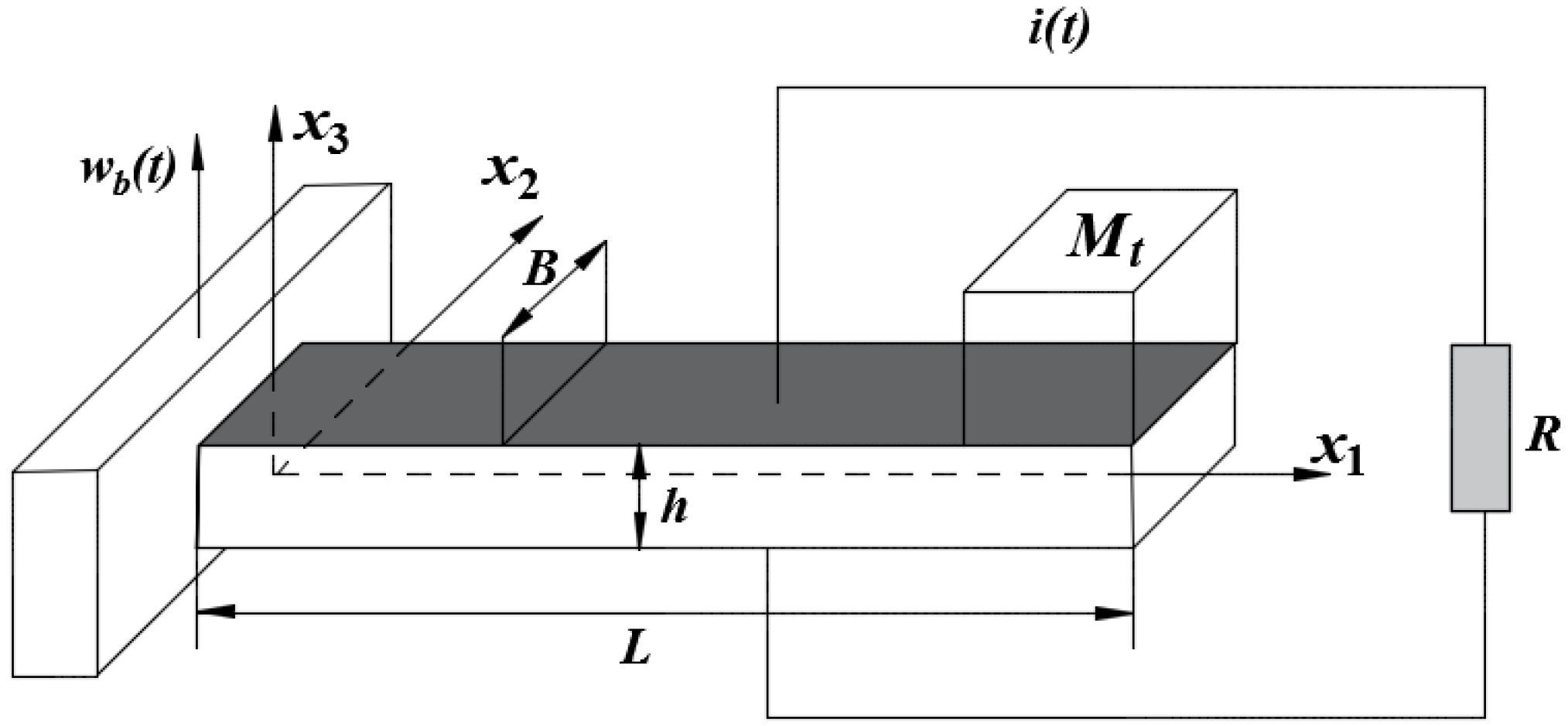
2. Electromechanical System and Mathematical Formation

The present study focuses on the vibration responses of a flexoelectric cantilever beam with length $L$, width $B$, thickness $h$, and a tip mass $M_{\mathrm{t}}$ as shown in Figure 1, in which the beam is coated by conductive electrodes on both upper and lower surfaces. We assumed the electrode layers were thin so that the effect of their stiffness on mechanical responses of the system was negligible. The coordinate system ($x_1,x_2, x_3$) is shown in Figure 1. The motion of the base for the flexoelectric beam was in the $x_3$ direction. With a transverse base excitation $w_{\mathrm{b}} \left(t\right)$, the cantilever beam vibrates in the bending mode. As a result of the dynamic strain gradient caused by vibration responses, the flexoelectric beam produces an alternating potential difference across the surface electrodes. These electrodes were connected to an external resistance (R) to quantify the electric potential and power output. Here, the internal electrical resistance of the flexoelectric beam was not taken into consideration since it can be regarded as a resistance connected in parallel to the external electrical load [37,41].

The generalized Hamilton’s variational principle for flexoelectric materials can be written as [32]

$$\mathsf{\delta }{\int }_0^T\left[K-G+W\right]\mathrm{d}t=0,$$

(1)

where $K,G, \mathrm{and}W$ are the total kinetic energy, total electric Gibbs free energy, and external work, respectively. In this study, the tip mass was regarded as a particle and the rotary inertia of the tip mass was not considered, which has less influence. Assuming no external body forces and electric field, for the flexoelectric cantilever beam showing in Figure 1, Equation (1) could be rewritten as

$$\mathsf{\delta }{\int }_0^T\mathrm{d}t{\int }_V\left[\frac{1}{2}\rho {\left|{\dot{w}}^m\right|}^2-g_1\right]\mathrm{d}V+\mathsf{\delta }{\int }_0^T\frac{1}{2}{M}_{\mathrm{t}}{\left|{\dot{w}}^m\right|}^2\mathrm{d}t{|}_{x_1=L}-{\int }_0^T\mathrm{d}t{\oint }_s\varpi \mathsf{\delta }\psi \mathrm{d}A=0,$$

(2)

where $\rho$ is density of this flexoelectric material, $w^m\left(x_1,t\right)=w_{\mathrm{b}}\left(t\right)+w\left(x_1,t\right)$ is the absolute displacement in the $x_3$ direction, $w=w\left(x_1,t\right)$ is the transverse displacement (relative to the base) of the neutral surface at point $x_1$, and $g_1$ is the general electric Gibbs free energy density. $\varpi \left(t\right)$ and $\psi \left(t\right)$ are the electric charge density and electric potential on the surface electrodes, which form the virtual work due to the moving charges on or out of the electrodes. It should be noted that the external work done by the surface hyper-stress tractions was ignored in this case.

For the flexoelectric material, the general electric Gibbs free energy density function $g_1$ can be expressed as [25,36]

$$g_1=\frac{1}{2}{\sigma }_{ij}{\epsilon }_{kl}+\frac{1}{2}{\sigma }_{ijk}{\epsilon }_{ij,k}-\frac{1}{2}{D}_i{E}_i,$$

(3)

where ${\sigma }_{ij}$ is the classical Cauchy stress tensor, ${\epsilon }_{ij}$ is the strain tensor, ${\sigma }_{ijk}$ is the higher-order stress tensor, $D_i$ is the electric displacement vector, and $E_i$ is the electric field vector. In this paper, the kinematics of the classical Euler–Bernoulli beam model was adopted to analyze the bending vibration of the flexoelectric beam for energy harvesting. The relative displacement field $\mathit{u}$ in the Euler–Bernoulli model is

$$\mathit{u}=\{-x_3\frac{\partial w}{\partial x_1},0,w\},$$

(4)

where the displacement in the $x_2$ direction is set to be zero as in the plane strain elasticity. With Equation (4) for infinitesimal deformation, the only non-zero strain component and its gradients are

$${\epsilon }_{11}=-x_3\frac{{\partial }^{2}w}{\partial x_1^2}, {\epsilon }_{11,3}=-\frac{{\partial }^{2}w}{\partial x_1^2}, {\epsilon }_{11,1}=-x_3\frac{{\partial }^{3}w}{\partial x_1^3},$$

(5)

where the stain gradient ${\epsilon }_{11,3}$ is essentially the bending curvature of the beam and ${\epsilon }_{11,1}$ is proportional to the gradient of curvature. The latter is typically small compared to the former in the Euler–Bernoulli beam model and may be neglected for a slender beam. For the same reason, only one component of the electric field, $E_3$, was considered due to the relatively small electric field $E_1$ in the length direction.

According to the constitutive equations of the flexoelectric beams, the non-zero stress, higher-order stress, and electric displacement are [25,32,36]

$$\{\begin{array}{c}{\sigma }_{11}=c_{1111}{\epsilon }_{11}-e_{311}{E}_3\\ {\sigma }_{113}=-{\mu }_{3113}{E}_3\\ D_3={\kappa }_{33}{E}_3+e_{311}{\epsilon }_{11}+{\mu }_{3113}{\epsilon }_{11,3}\end{array},$$

(6)

where ${\sigma }_{113}$ is defined as the higher order stress or the moment stress [25,36], which is induced by the electric field due to the flexoelectric effect, $c_{1111}$ is an elastic modulus, $e_{311}$ is a piezoelectric coefficient, ${\mu }_{3113}$ is a flexoelectric coefficient, and ${\kappa }_{33}$ is a dielectric coefficient.

In the absence of free body charges, Gauss’s law of electrostatics leads to

$$\frac{{\partial }^2\Phi }{\partial x_3^2}=\frac{e_{311}}{{\kappa }_{33}}{\epsilon }_{11,3},$$

(7)

where $\Phi =\Phi \left(x_1,x_3,t\right)$ is the electric potential of the beam and is related to the electric field by $E_3=-\frac{\partial \Phi }{\partial x_3}$. Considering the surface electrical boundary conditions $\Phi \left(x_1, x_3=\frac{h}{2},t\right)={\psi }_1\left(x_1, t\right)$ and $\Phi \left(x_1, x_3=-\frac{h}{2},t\right)={\psi }_2\left(x_1, t\right)$, the dynamic electric potential $\Phi$ and dynamic electric field $E_3$ can be obtained from Equation (7) as

$$\Phi \left(x_1, x_3,t\right)=\frac{e_{311}}{2{\kappa }_{33}}\frac{{\partial }^{2}w}{\partial x_1^2}\left(\frac{h^2}{4}-x_3^2\right)+\left(\frac{1}{2}+\frac{x_3}{h}\right)\psi \left(x_1, t\right)+{\psi }_2\left(x_1, t\right),$$

(8)

$$E_3=-\frac{e_{311}}{{\kappa }_{33}}{\epsilon }_{11}-\frac{\psi \left(x_1, t\right)}{h},$$

(9)

where $\psi \left(x_1, t\right)={\psi }_1\left(x_1, t\right)-{\psi }_2\left(x_1, t\right)$ is the potential difference or voltage between the both surface electrodes. Substituting Equation (9) into Equation (6), the electric displacement, stress, and higher order stress could be expressed as

$$\{\begin{array}{c}{D}_3={\mu }_{3113}{\epsilon }_{11,3}-{\kappa }_{33}\frac{\psi }{h}\\ {\sigma }_{11}=\left(c_{1111}+\frac{e_{311}^2}{{\kappa }_{33}}\right){\epsilon }_{11}+e_{311}\frac{\psi }{h}\\ {\sigma }_{113}=\frac{{\mu }_{3113}{e}_{311}}{{\kappa }_{33}}{\epsilon }_{11}+{\mu }_{3113}\frac{\psi }{h}\end{array}.$$

(10)

Then, by Equation (3), the electric Gibbs free energy density is obtained as follows [36]:

$$g_1=\frac{1}{2}\left(c_{1111}+\frac{e_{311}^2}{{\kappa }_{33}}\right){\epsilon }_{11}^2+\frac{e_{311}{\mu }_{3113}}{{\kappa }_{33}}{\epsilon }_{11}{\epsilon }_{11,3}+{\mu }_{3113}{\epsilon }_{11,3}\frac{\psi }{h}-\frac{1}{2}{\kappa }_{33}\frac{{\psi }^2}{h^2}.$$

(11)

Using Equations (5) and (6), the variational expression of general electric Gibbs free energy can be written as [36]

$$\begin{array}{c}\mathsf{\delta }{\int }_0^T\mathrm{d}t{\int }_V{g}_1\mathrm{d}V={\int }_0^T{\int }_0^L\left\{\left[G_{\mathrm{p}}\frac{{\partial }^{4}w}{\partial x_1^4}-{\mu }_{3113}B\frac{{\partial }^2\psi }{\partial x_1^2}\right]\mathsf{\delta }w-\left[{\mu }_{3113}B\frac{{\partial }^{2}w}{\partial x_1^2}+{\kappa }_{33}\frac{\psi B}{h}\right]\mathsf{\delta }\psi \right\}\mathrm{d}{x}_1\mathrm{d}t+\hfill \\ {\int }_0^T\left\{G_{\mathrm{p}}\frac{{\partial }^{2}w}{\partial x_1^2}-{\mu }_{3113}B\psi \right\}\mathsf{\delta }\left(\frac{\partial w}{\partial x_1}\right){|}_{x_1=L}\mathrm{d}t-{\int }_0^T\left\{G_{\mathrm{p}}\frac{{\partial }^{3}w}{\partial x_1^3}\right\}\mathsf{\delta }w{|}_{x_1=L}\mathrm{d}t,\hfill \end{array}$$

(12)

where $G_{\mathrm{p}}=\frac{B{h}^3}{12}\left(c_{1111}+\frac{e_{311}^2}{{\kappa }_{33}}\right)$ is the effective bending rigidity of the piezoelectric beam. It should be noted that the present effective bending rigidity is quite different from the previous result in [37], where the effective bending rigidity was derived from an internal energy density function. The effective bending rigidity in [37] depends on the flexoelectricity of the material and becomes negative when the beam thickness is small (~several nanometers). In contrast, the effective bending rigidity $G_{\mathrm{p}}$ in the present model remains positive, independent of the flexoelectric coefficients.

Substituting Equation (12) into Equation (2), the generalized Hamilton’s variational equation of the flexoelectric beam can be rewritten as

$$\begin{array}{c}{\int }_0^T\mathrm{d}t\left\{Bh{\int }_0^L\rho \left(\ddot{w}+{\ddot{w}}_{\mathrm{b}}\right)\mathsf{\delta }w\mathrm{d}{x}_1+M_{\mathrm{t}}{\ddot{w}}_{\mathrm{b}}\delta \left(x_1-L\right)\mathsf{\delta }w\right\}+{\int }_0^T\mathrm{d}t{\int }_0^L\{[G_{\mathrm{p}}\frac{{\partial }^{4}w}{\partial x_1^4}-\\ {\mu }_{3113}B\frac{{\partial }^2\psi }{\partial x_1^2}]\mathsf{\delta }w-\left[{\mu }_{3113}B\frac{{\partial }^{2}w}{\partial x_1^2}+{\kappa }_{33}B\frac{\psi }{h}\right]\mathsf{\delta }\psi \}\mathrm{d}{x}_1\mathrm{d}t+{\int }_0^T\{G_{\mathrm{p}}\frac{{\partial }^{2}w}{\partial x_1^2}-\\ {\mu }_{3113}B\psi \}\mathsf{\delta }\left(\frac{\partial w}{\partial x_1}\right){|}_{x_1=L}\mathrm{d}t-{\int }_0^T\left\{G_{\mathrm{p}}\frac{{\partial }^{3}w}{\partial x_1^3}-M_{\mathrm{t}}\frac{{\partial }^{2}w}{\partial t^2}\right\}\mathsf{\delta }w{|}_{x_1=L}\mathrm{d}t-{\int }_0^T\mathrm{d}t{\int }_0^{L}B\varpi \mathsf{\delta }\psi \mathrm{d}{x}_1\mathrm{d}t=\\ 0,\end{array}$$

(13)

where $\delta \left(x_1\right)$ is the Dirac delta function. In deducing Equation (13), the following result has been used

$$\mathsf{\delta }{\int }_0^T\frac{1}{2}{M}_{\mathrm{t}}{\left|{\dot{w}}^m\right|}^2\mathrm{d}t{|}_{x_1=L}=-{\int }_0^T{M}_{\mathrm{t}}{\ddot{w}}_b\delta \left(x_1-L\right)\mathsf{\delta }w\mathrm{d}t-{\int }_0^T{M}_{\mathrm{t}}\ddot{w}{|}_{x_1=L}\mathsf{\delta }w\mathrm{d}t.$$

(14)

Due to the arbitrariness of $\mathsf{\delta }w$ in Equation (13), the electromechanically-coupled dynamic governing equation of the flexoelectric beam can be obtained as

$$G_{\mathrm{p}}\frac{{\partial }^{4}w}{\partial x_1^4}-{\mu }_{3113}B\frac{{\partial }^2\psi }{\partial x_1^2}+\left[m+M_{\mathrm{t}}\delta \left(x_1-L\right)\right]\frac{{\partial }^2{w}_b}{\partial t^2}+m\frac{{\partial }^{2}w}{\partial t^2}=0,$$

(15)

where $m=\rho Bh$ is the mass of per unit length of beam.

Similarly, due to the arbitrariness of $\mathsf{\delta }\psi$ in Equation (13), we obtain

$${\int }_0^L({\mu }_{3113}\frac{{\mathrm{d}}^{2}w}{\mathrm{d}{x}_1^2}+{\kappa }_{33}\frac{\psi }{h}+\varpi )\mathrm{d}{x}_1=0.$$

(16)

When the external loading resistor $R$ is connected into the surface electrodes, the electric current $\frac{\psi }{R}$ must be equal to the time rate of change of the average output positive charges, i.e., $-\frac{1}{h}{\int }_V\dot{\varpi }\mathrm{d}V$. Using Equation (16), from Gauss’s law [37,41,42], the electromechanically-coupled electrical circuit equation with flexoelectric effect can be written as

$${\kappa }_{33}BL\frac{\dot{\psi }}{h}+\frac{\psi }{R}=-{\mu }_{3113}B{\frac{{\partial }^{2}w}{\partial x_1\partial t}|}_{x_1=L},$$

(17)

where $\psi$ is assumed to be independent of $x_1$. In addition, the boundary conditions are obtained from Equation (13) as

$$\{\begin{array}{c}{G}_{\mathrm{p}}{\frac{{\partial }^{2}w}{\partial x_1^2}|}_{x_1=L}={\mu }_{3113}B\psi \\ G_{\mathrm{p}}{\frac{{\partial }^{3}w}{\partial x_1^3}|}_{x_1=L}=M_{\mathrm{t}}{\frac{{\partial }^{2}w}{\partial t^2}|}_{x_1=L}\end{array}.$$

(18)

Apparently, the flexoelectric effect induces an effective bending moment at the end of the beam, whereas the inertia of the tip mass induces a shear force at the end.

3. Closed-Form Expressions of Electromechanical Frequency Response Functions

3.1. Electromechanical Governing Equations in Modal Coordinates

In the real vibration structures, damping is an important part of the system and also a very complicated problem. Here we take two types of damping mechanisms into account in order to emphasize the flexoelectric effect. These two types of damping are called viscous air (or external) damping and Kelvin–Voigt (or strain-rate) damping [37,42]. With the damping effects, the electromechanical dynamic Equation (15) becomes

$$G_{\mathrm{p}}\frac{{\partial }^{4}w}{\partial x_1^4}-{\mu }_{3113}B\frac{{\partial }^2\psi }{\partial x_1^2}+c_{\mathrm{s}}\frac{{\partial }^{5}w}{\partial x_1^4\partial t}+c_{\mathrm{a}}\frac{\partial w}{\partial t}+\left[m+M_{\mathrm{t}}\delta \left(x_1-L\right)\right]\frac{{\partial }^2{w}_{\mathrm{b}}}{\partial t^2}+m\frac{{\partial }^{2}w}{\partial t^2}=0,$$

(19)

where $c_{\mathrm{a}}$ is the viscous air damping coefficient and $c_{\mathrm{s}}$ is the strain-rate damping coefficient [42]. Viscous air damping is a simple way of modeling the force acting on the beam due to the air particles displaced during vibration, while strain-rate damping accounts for the structural damping due to energy dissipation of the beam material. Both of them satisfy the proportional damping criterion and they are mathematically convenient for the modal analysis [42].

Based on the proportional damping assumption, the vibration response of the flexoelectric cantilever beam can be represented as an absolutely and uniformly convergent series of eigenfunctions as

$$w\left(x_1,t\right)={\sum }_{r=1}^{\infty }{\varnothing }_r\left(x_1\right){\eta }_r\left(t\right),$$

(20)

where ${\varnothing }_r\left(x\right)$ is the mass normalized eigenfunction of the rth vibrational mode, which satisfies the mechanical and the short circuit electrical conditions, and ${\eta }_r\left(t\right)$ is the modal mechanical response coefficient in the modal coordinates. For the piezoelectric or flexoelectric Euler–Bernoulli cantilever beams, the eigenfunctions ${\varnothing }_r\left(x\right)$ can be obtained from the corresponding undamped free vibration problem [41]

$${\varnothing }_r\left(x_1\right)=C_r\left[\cos \frac{{\beta }_r}{L}{x}_1-\cos \mathrm{h}\frac{{\beta }_r}{L}{x}_1+{\zeta }_r\left(\sin \frac{{\beta }_r}{L}{x}_1-\sin \mathrm{h}\frac{{\beta }_r}{L}{x}_1\right)\right],$$

(21)

where ${\zeta }_r$ is

$${\zeta }_r=\frac{\sin {\beta }_r-\sin \mathrm{h}{\beta }_r+{\beta }_r\frac{M_{\mathrm{t}}}{mL}\left(\cos {\beta }_r-\sin \mathrm{h}{\beta }_r\right)}{\cos {\beta }_r+\cos \mathrm{h}{\beta }_r-{\beta }_r\frac{M_{\mathrm{t}}}{mL}\left(\sin {\beta }_r-\sin \mathrm{h}{\beta }_r\right)},$$

(22)

and ${\beta }_r$ is the rth root of the transcendental characteristic equation

$$1+\cos {\beta }_r\cos \mathrm{h}{\beta }_r+{\beta }_r\frac{M_{\mathrm{t}}}{mL}\left(\cos {\beta }_r\sin \mathrm{h}{\beta }_r-\sin {\beta }_r\cos \mathrm{h}{\beta }_r\right)=0.$$

(23)

In Equation (21), the constant $C_r$ is the modal amplitude constant, which could be solved by normalizing the eigenfunctions using the following orthogonality condition [33]

$${\int }_0^L{\varnothing }_r\left(x_1\right)m{\varnothing }_s\left(x_1\right)\mathrm{d}{x}_1+{\varnothing }_r\left(L\right)M_{\mathrm{t}}{\varnothing }_s\left(L\right)={\delta }_{rs},$$

(24)

where ${\delta }_{rs}$ is Kronecker delta, defined as being equal to unity for $s=r$ and equal to zero for $s\ne r$. It should be noted that the undamped natural frequency of the $r\mathrm{th}$ vibration mode in the short circuit condition is

$${\omega }_r={\beta }_r^2\sqrt{\frac{G_{\mathrm{p}}}{m{L}^4}}.$$

(25)

It is important to mention that the electric potential difference between the two surface electrodes due to the flexoelectric effect is a function of time t and as a result, the spatial derivative of $\psi$ would vanish in Equation (19). To include the flexoelectric effect in the governing Equation (19), Erturk and Inman [41] assumed that $\psi =\psi \left(x_1,t\right)=V\left(t\right)\left[H\left(x_1\right)-H\left(x_1-L\right)\right]$, where $V\left(t\right)$ is the output voltage and $H\left(x\right)$ is the Heaviside function.

To investigate the dynamic response of the system, the mode-superposition method was adopted to solve the damped flexoelectric cantilever beam with the tip mass. Substituting the modified electric potential expression and Equation (20) into Equation (19) and using the orthogonality condition (24), the electromechanical coupling dynamic governing equation of the damped flexoelectric beams in modal coordinates can be written as

$$\frac{{\mathrm{d}}^2{\eta }_r\left(t\right)}{\mathrm{d}{t}^2}+{\omega }_r^2{\eta }_r\left(t\right)+\frac{\mathrm{d}{\eta }_r\left(t\right)}{\mathrm{d}t}2{\xi }_r{\omega }_r={\int }_0^L{\mu }_{3113}BV\left(t\right){\varnothing }_r\left(x_1\right)\left[\frac{\mathrm{d}\delta \left(x_1\right)}{\mathrm{d}{x}_1}-\frac{\mathrm{d}\delta \left(x_1-L\right)}{\mathrm{d}{x}_1}\right]\mathrm{d}{x}_1-m\left[\frac{{\mathrm{d}}^2{w}_{\mathrm{b}}\left(t\right)}{\mathrm{d}{t}^2}{\int }_0^L{\varnothing }_r\left(x_1\right)\mathrm{d}{x}_1\right]-M_{\mathrm{t}}{\varnothing }_r\left(L\right)\frac{{\mathrm{d}}^2{w}_{\mathrm{b}}\left(t\right)}{\mathrm{d}{t}^2},$$

(26)

where ${\xi }_r$ is defined as the modal damping ratio of rth which include the viscous air damping part $c_{\mathrm{a}}$ and the strain-rate damping part $c_{\mathrm{s}}$ [37,43]. Commonly, in experimental modal analysis practice, one can identify the modal damping ratio ${\xi }_r$ directly from the frequency response or time-domain measurements, which avoids the requirement of defining and obtaining the physical damping terms $c_{\mathrm{s}}$ and $c_{\mathrm{a}}$ [41]. Here, the $n\mathrm{th}$ derivative of the Dirac delta function satisfies the condition as follows

$${\int }_{-\infty }^{+\infty }\frac{{\mathrm{d}}^n\delta \left(x-x_0\right)}{\mathrm{d}{x}^n}\gamma \left(x\right)\mathrm{d}x={\left(-1\right)}^n\frac{{\mathrm{d}}^n\gamma \left(x\right)}{\mathrm{d}{x}^n}{|}_{x=x_0}.$$

(27)

With Equation (27), the modal equation can be written as

$$\frac{{\mathrm{d}}^2{\eta }_r\left(t\right)}{\mathrm{d}{t}^2}+{\omega }_r^2{\eta }_r\left(t\right)+\frac{\mathrm{d}{\eta }_r\left(t\right)}{\mathrm{d}t}2{\xi }_r{\omega }_r-{\mu }_{3113}BV\left(t\right)\frac{\mathrm{d}{\varnothing }_r\left(x_1\right)}{\mathrm{d}{x}_1}{|}_{x_1=L}=f_r\left(t\right),$$

(28)

where $f_r\left(t\right)$ is the modal mechanical force function corresponding to the base excitation

$$f_r\left(t\right)=-m\left[\frac{{\mathrm{d}}^2{w}_{\mathrm{b}}\left(t\right)}{\mathrm{d}{t}^2}{\int }_0^L{\varnothing }_r\left(x_1\right)\mathrm{d}{x}_1\right]-M_{\mathrm{t}}{\varnothing }_r\left(L\right)\frac{{\mathrm{d}}^2{w}_{\mathrm{b}}\left(t\right)}{\mathrm{d}{t}^2}.$$

(29)

Similarly, substituting Equation (20) into Equation (17), the modal circuit equation can be obtained as

$$\frac{{\kappa }_{33}BL}{h}\frac{\mathrm{d}V\left(t\right)}{\mathrm{d}t}+\frac{V\left(t\right)}{R}=-{\sum }_{r=1}^{\infty }{K}_r\frac{\mathrm{d}{\eta }_r\left(t\right)}{\mathrm{d}t},$$

(30)

where $K_r={\mu }_{3113}B\frac{\mathrm{d}{\varnothing }_r\left(x\right)}{\mathrm{d}x}{|}_{x_1=L}$.

3.2. Closed-Form Frequency Response Functions

The motion of the base for the cantilever is typically represented by the translational displacement in the transverse direction with superimposed small rotational displacement. Here, only the translational displacement was considered. Assume the vibration of the base to be a harmonic excitation with a frequency $\omega$, i.e., $w_{\mathrm{b}}\left(t\right)=W_0{\mathrm{e}}^{\mathrm{j}\omega t}$, where $W_0$ is the amplitude of the base vibration and $\mathrm{j}=\sqrt{-1}$ is the imaginary unit. Then, the modal mechanical force can be written as $f_r\left(t\right)=F_r{\mathrm{e}}^{\mathrm{j}\omega t}$, where the amplitude of the modal mechanical force function could be expressed as

$$F_r=W_0{\omega }^2\left[m{\int }_0^L{\varnothing }_r\left(x_1\right)\mathrm{d}{x}_1+M_{\mathrm{t}}{\varnothing }_r\left(L\right)\right].$$

(31)

With the small deformation and linear system assumption, the modal mechanical and electrical responses were in steady state and also harmonic with the same frequency as the base excitation. Thus, the modal mechanical response and voltage response can be written as ${\eta }_r\left(t\right)=H_r{e}^{\mathrm{j}\omega t}$ and $V\left(t\right)=v{\mathrm{e}}^{\mathrm{j}\omega t}$, respectively, in which both $H_r$ and $v$ are generally complex valued. Then, Equations (28) and (30) lead to

$$\{\begin{array}{c}\left[\left({\omega }_r^2-{\omega }^2\right)+2{\xi }_r{\omega }_r\mathrm{j}\omega \right]H_r-v{K}_r=F_r,\\ \left(\frac{{\kappa }_{33}BL}{h}\mathrm{j}\omega +\frac{1}{R}\right)v+j\omega {\displaystyle {\displaystyle \sum }_{r=1}^{\infty }}{K}_r{H}_r=0.\end{array}$$

(32)

Solving Equation (32), $H_r$ and $v$ are obtained explicitly. The analytical modal expressions of voltage $V$ and mechanical response ${\eta }_r\left(t\right)$ can be obtained as follows

$$V\left(t\right)=-\frac{\mathrm{j}\omega {\sum }_{r=1}^{\infty }\frac{K_r{F}_r}{\left({\omega }_r^2-{\omega }^2\right)+2\mathrm{j}\omega {\xi }_r{\omega }_r}}{\left(\frac{1}{R}+\frac{{\kappa }_{33}BL}{h}\mathrm{j}\omega \right)+{\sum }_{r=1}^{\infty }\frac{\mathrm{j}\omega K_r^2}{\left({\omega }_r^2-{\omega }^2\right)+2\mathrm{j}\omega {\xi }_r{\omega }_r}}{\mathrm{e}}^{\mathrm{j}\omega t},$$

(33)

$${\eta }_r\left(t\right)=\left[\frac{F_r}{\left({\omega }_r^2-{\omega }^2\right)+2\mathrm{j}\omega {\xi }_r{\omega }_r}+V\left(t\right)\frac{K_r}{\left({\omega }_r^2-{\omega }^2\right)+2\mathrm{j}\omega {\xi }_r{\omega }_r}\right]{\mathrm{e}}^{\mathrm{j}\omega t}.$$

(34)

We can then substitute ${\eta }_r\left(t\right)$ into Equation (20) to obtain the deflection response $w\left(x_1,t\right)$.

4. Numerical Results and Discussion

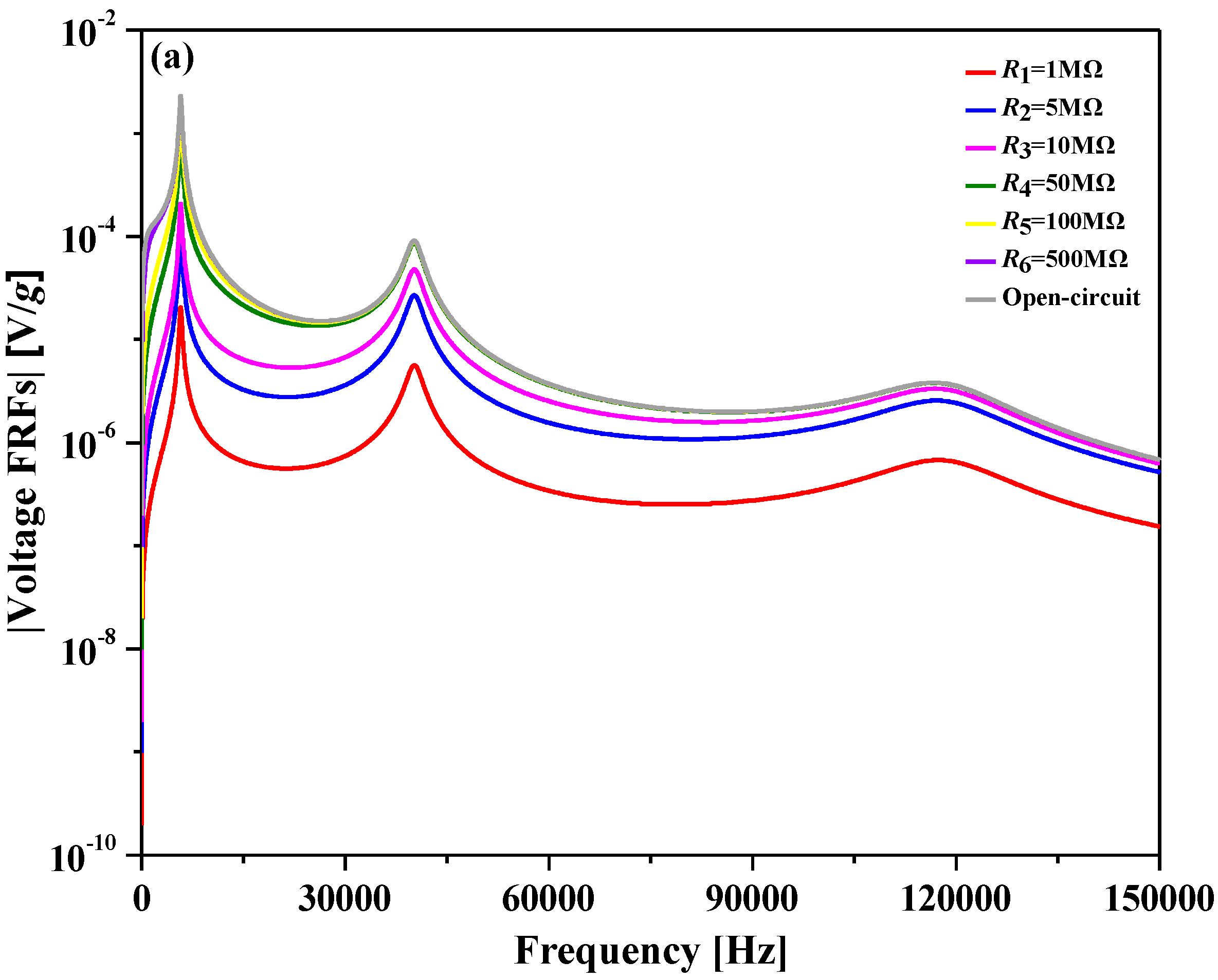
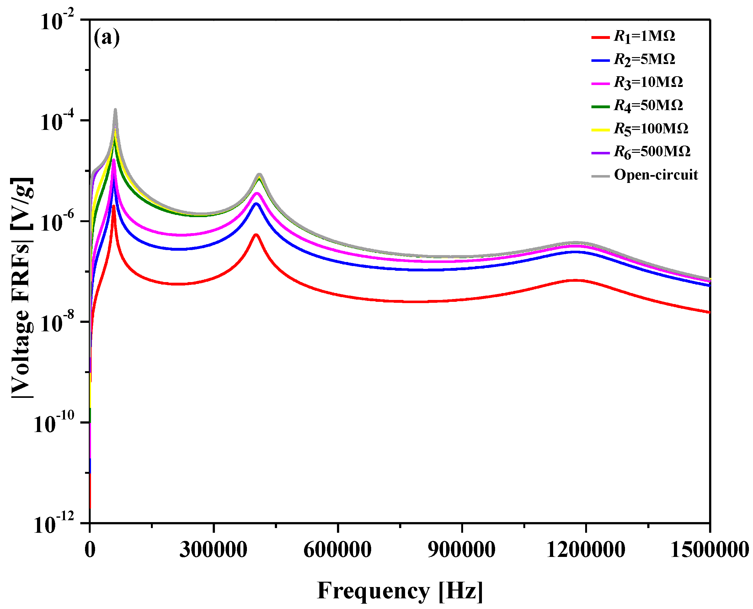
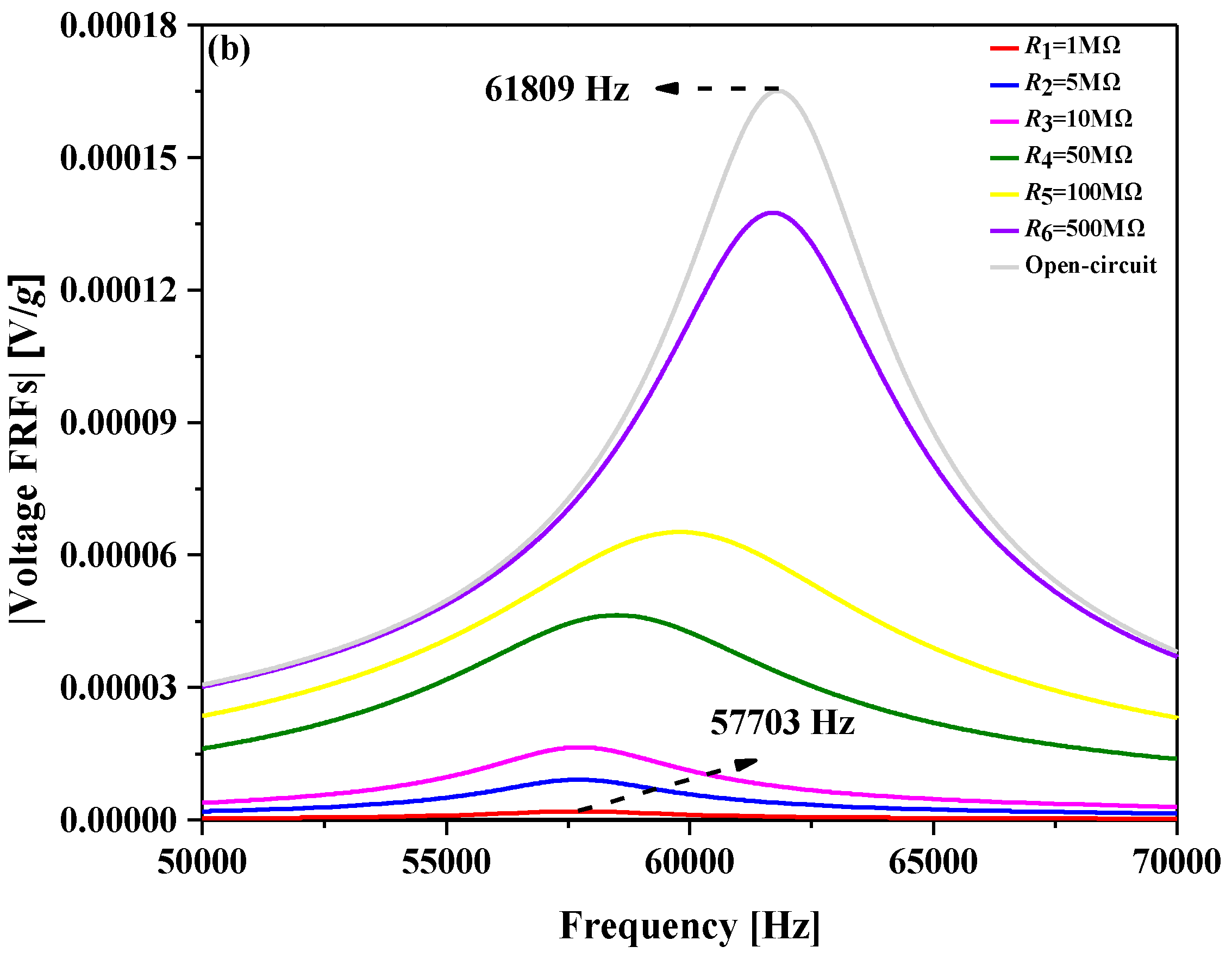
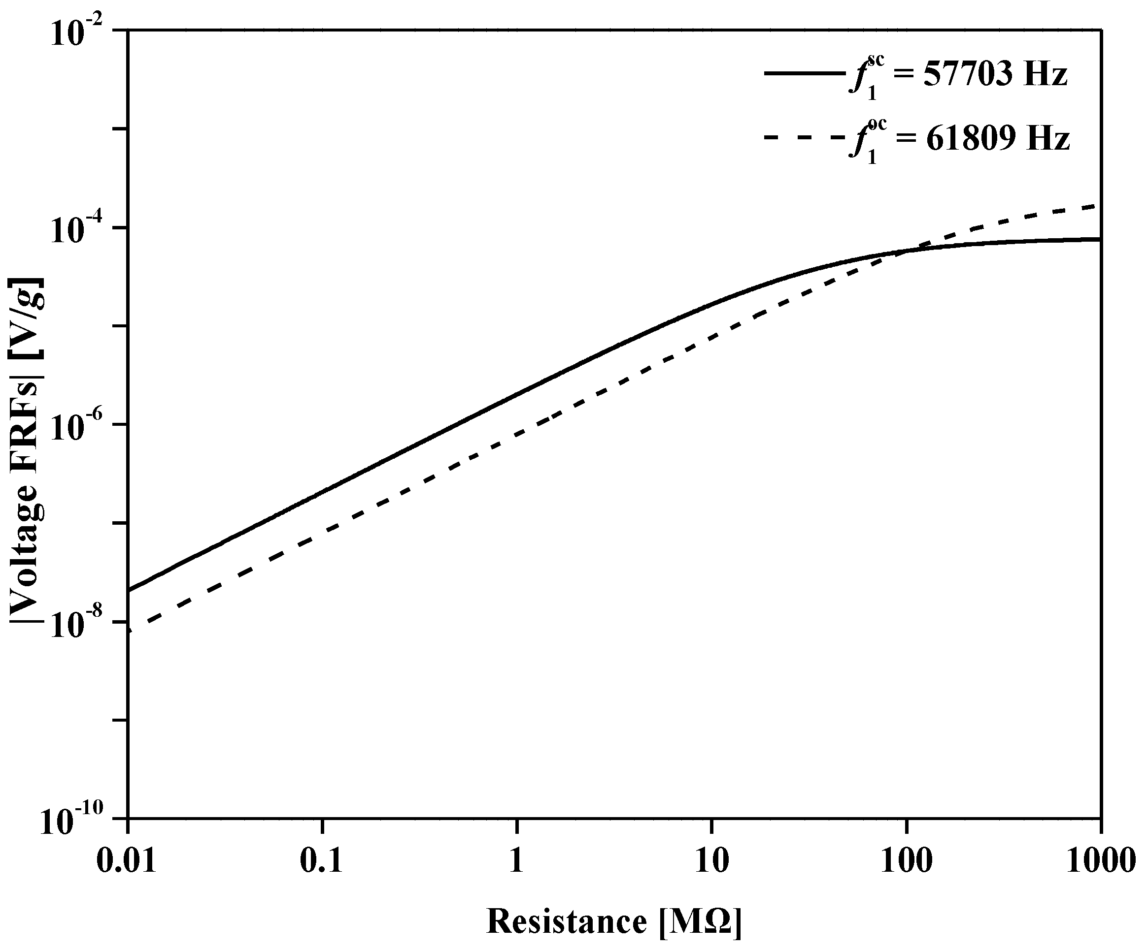
In this section, polyvinylidene difluoride (PVDF) is taken as an example material to demonstrate the effects of size and the electric resistance on flexoelectric energy harvesting. The PVDF is a flexible piezoelectric polymer material, which has the following properties: mass density $\rho =1.78\times {10}^3\mathrm{kg}/{\mathrm{m}}^3$, elastic modulus $c_{1111}=3.7\mathrm{GPa}$ [37], piezoelectric coefficient $e_{311}=-0.01 \mathrm{N}/\mathrm{V}·\mathrm{m}$, dielectric permittivity ${\kappa }_{33}=8.15\times {10}^{-11} {\mathrm{C}}^2/\left(\mathrm{N}·{\mathrm{m}}^2\right)$, and flexoelectric coefficient ${\mu }_{3113}=2.3\times {10}^{-2}\mathsf{\mu }\mathrm{C}/\mathrm{m}$ [44]. In all analyses, the length/width/thickness aspect ratio of the beam, $100:10:1$, was maintained constant over the entire frequency range. For the tip mass, $M_{\mathrm{t}}=0.2\times m\times L$ was chosen in the following simulations. The damping ratios were given by ${\xi }_1={\xi }_2=0.0285$, with which the two damping coefficients ($c_{\mathrm{s}}$ and $c_{\mathrm{a}}$) can be obtained [42]. For convenience, all the simulation results are given in form of FRFs, which were normalized by the base excitation acceleration ${\ddot{w}}_{\mathrm{b}}=-{\omega }^2{W}_0{\mathrm{e}}^{\mathrm{j}\omega t}$.

4.1. Voltage FRFs

The voltage FRFs in Equation (33) can be re-written as

$$\frac{V\left(t\right)}{-{\omega }^2{W}_0{\mathrm{e}}^{\mathrm{j}\omega t}}=-\frac{{\sum }_{r=1}^3\frac{\mathrm{j}\omega K_r{\lambda }_r}{\left({\omega }_r^2-{\omega }^2\right)+2\mathrm{j}\omega {\xi }_r{\omega }_r}}{\left(\frac{1}{R}+\frac{{\kappa }_{33}BL}{h}\mathrm{j}\omega \right)+{\sum }_{r=1}^3\frac{\mathrm{j}\omega K_r^2}{\left({\omega }_r^2-{\omega }^2\right)+2\mathrm{j}\omega {\xi }_r{\omega }_r}},$$

(35)

where ${\lambda }_r=-m{\int }_0^L{\varphi }_r\left(x_1\right)\mathrm{d}x-M_{\mathrm{t}}{\varphi }_r\left(L\right)$. In subsequent simulations, the first three modes were calculated and discussed.

Figure 2 shows the multi-mode voltage FRFs of the flexoelectric beam with a thickness of $3\mathsf{\mu }\mathrm{m}$ for arbitrary frequency excitations. By increasing the loading resistance from a small value ($R=1 \mathrm{M}\mathsf{\Omega }$) to open circuit ($R=1 \mathrm{G}\mathsf{\Omega }$, as an approximation for the open circuit condition) conditions, the voltage output increases monotonically at all frequencies. From the response around the first mode in Figure 2b, we found the resonance frequency (~5770 Hz) was almost identical for all loading resistances. This indicates that the resonance frequencies were insensitive to the variation of the loading resistances in the flexoelectric beam. It should be noted that, based on the present linear model, the electromechanical responses would perform well only in the narrow frequency zone close to the natural frequency. In practice, methods for performance enhancement have been developed by the use of nonlinearity [45,46,47,48] and multimodal techniques [49,50,51,52].

When the flexoelectric beam was shrunk proportionally to $0.3\mathsf{\mu }\mathrm{m}$ in thickness, the voltage FRFs are plotted in Figure 3. It is clear to observe that the resonance frequency increases about 10 times compared to Figure 2 for the beam with thickness $3\mathsf{\mu }\mathrm{m}$, as expected by Equation (25). The enlarged view of the voltage FRFs near the first mode is shown in Figure 3b. It is interesting to see that the resonance frequency corresponding to the peak voltage FRFs shifts from the short circuit resonance frequency ($f_1^{\mathrm{sc}}=\mathrm{57,703} \mathrm{Hz}$) to the open circuit resonance frequency ($f_1^{\mathrm{oc}}=\mathrm{61,809} \mathrm{Hz}$) as the loading resistance increases. The short circuit resonance frequencies can be obtained by solving Equations (23) and (25), and the open circuit resonance frequencies can be predicted using the previous result [53]. This result indicates that the resonance frequency of a small-scale flexoelectric energy harvesting device is dependent on the external loading resistance. Indeed, a resonance frequency shift was observed previously in piezoelectric and flexoelectric energy harvesting devices [37,41,42,54].

Figure 4 gives the variation of the voltage FRFs for the external excitations at the short circuit resonance frequency and the open circuit resonance frequency, respectively. In log-log scale, both voltage outputs increase with increasing loading resistance, and trend to constant values at large loading resistance. The two curves intersect at a point where the loading resistance is about $97 \mathrm{M}\mathsf{\Omega }$. If the loading resistance was greater than 97 $\mathrm{M}\mathsf{\Omega }$, the voltage output at the open circuit resonance frequency was larger because the system was closer to the open circuit condition. On the other hand, for lower loading resistance, the voltage output at the short circuit resonance frequency was larger. Therefore, when the loading resistance was larger than this special value, choosing the open circuit resonance frequency as the external excitation frequency would be optimal for the voltage FRFs since the system was closer to the open circuit condition and vice versa.

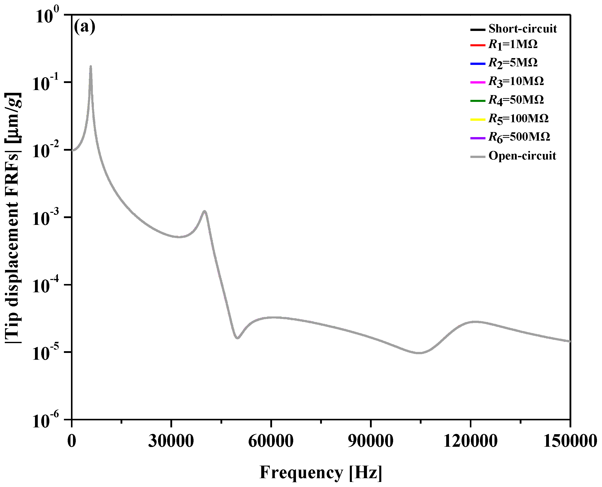
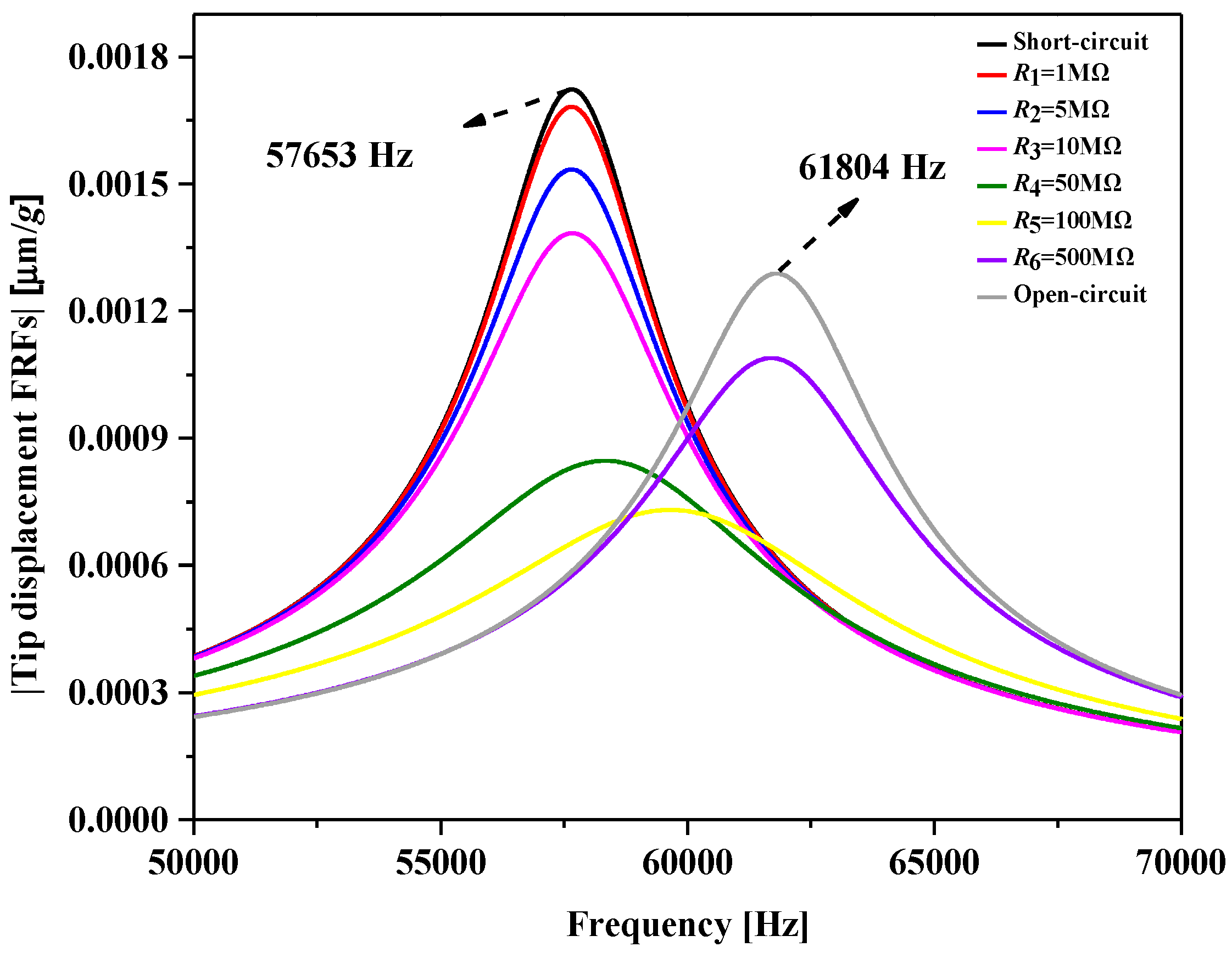
4.2. Tip Displacement FRFs

The multi-modes expression for the tip displacement FRFs can be obtained as

$$\frac{w\left(L,t\right)}{-{\omega }^2{W}_0{\mathrm{e}}^{\mathrm{j}\omega t}}={\sum }_{r=1}^3\left\{\left[{\lambda }_r-\frac{{\sum }_{r=1}^3\frac{\mathrm{j}\omega K_r{\lambda }_r}{\left({\omega }_r^2-{\omega }^2\right)+2\mathrm{j}\omega {\xi }_r{\omega }_r}}{\left(\frac{1}{R}+\frac{{\kappa }_{33}BL}{h}\mathrm{j}\omega \right)+{\sum }_{r=1}^3\frac{\mathrm{j}\omega K_r^2}{\left({\omega }_r^2-{\omega }^2\right)+2\mathrm{j}\omega {\xi }_r{\omega }_r}}{K}_r\right]\frac{{\varnothing }_r\left(L\right)}{\left({\omega }_r^2-{\omega }^2\right)+2\mathrm{j}\omega {\xi }_r{\omega }_r}\right\}.$$

(36)

The tip displacement FRFs of the beam with the excitation frequency for the $3 \mathsf{\mu }\mathrm{m}$ thickness beam with the tip mass $M_{\mathrm{t}}$ are plotted in Figure 5. For the different load resistances, the values of the tip displacement FRFs were almost equal. In other words, the tip displacement FRFs were independent of the loading resistance. It is interesting to see that in Figure 5, there are two small anti-resonance frequencies between mode 2 and mode 3, which is different from the result of piezoelectric energy harvesting devices [42]. In the piezoelectric case without the tip mass, there was just one intense mechanical anti-resonance frequency between mode 2 and mode 3.

Figure 6 plots the tip displacement FRFs of the $0.3 \mathsf{\mu }\mathrm{m}$ thickness beam with the tip mass $M_{\mathrm{t}}$ near the first mode. Comparing Figure 5 and Figure 6, it is clear to observe that the tip displacement FRFs depend on the external loading resistance for the small scale flexoelectric energy harvesting. The significant resonance frequency shift from $f_1^{\mathrm{sc}}$ to $f_1^{\mathrm{oc}}$ could be observed with increasing load resistance. Apparently, at a small scale, the electromechanical coupling of the flexoelectric energy harvesting is enhanced, which was not the case for the piezoelectric energy harvesting. It is interesting to see that the peak amplitude of the tip displacement FRFs first decreases and then increases with increasing load resistance. This was due to the power dissipation as a result of Joule heating in the electrical domain with the finite values of load resistance [42]. This phenomenon can also be found in the case of piezoelectric energy harvesting systems.

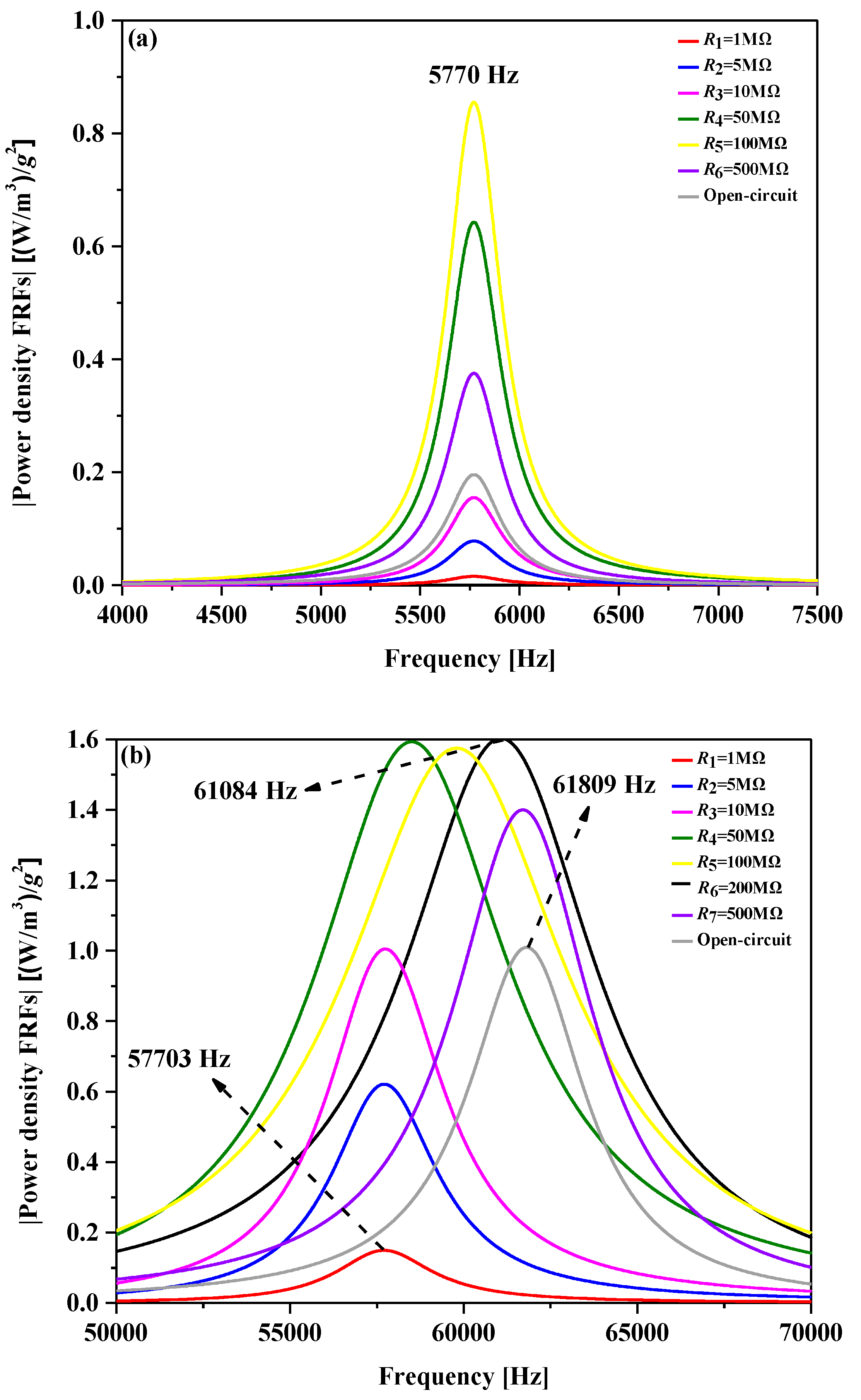
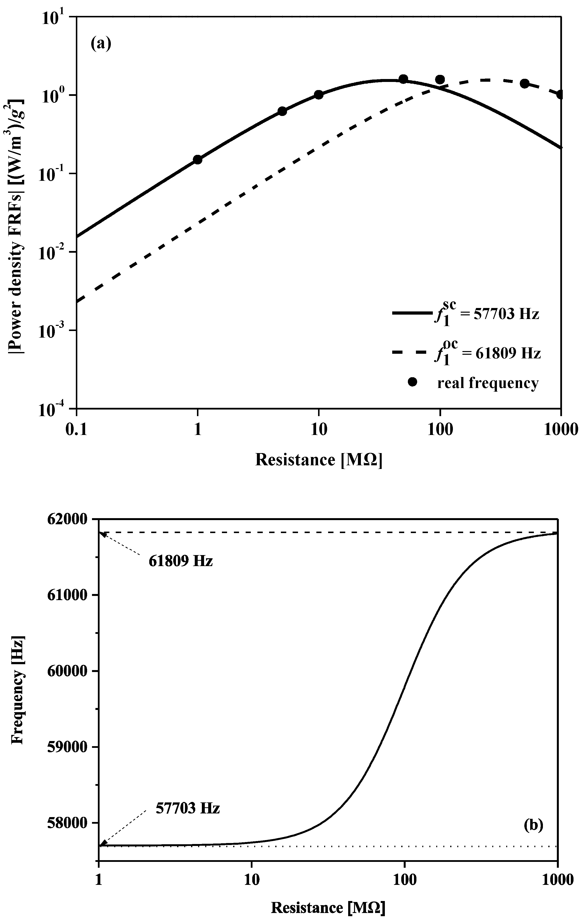
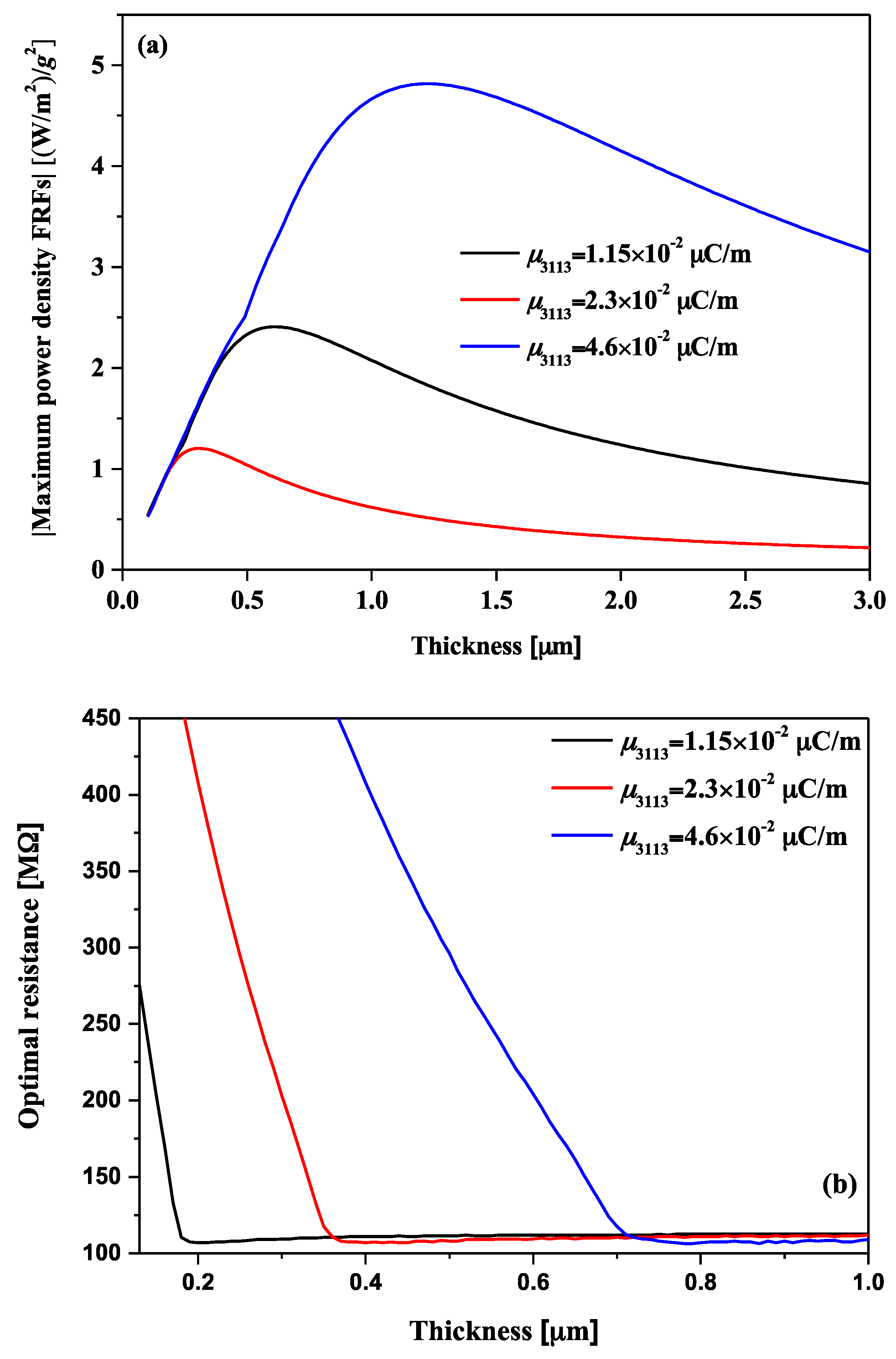
4.3. Power Density FRFs

For energy harvesting, the power density is an important measure of performance. In the case of the flexoelectric beam, the power density FRFs could be expressed as follows

$$\frac{P_{\mathrm{d}}\left(t\right)}{-{\omega }^2{W}_0{\mathrm{e}}^{\mathrm{j}\omega t}}={\left[\frac{{\sum }_{r=1}^3\frac{-\mathrm{j}\omega K_r{\lambda }_r}{\left({\omega }_r^2-{\omega }^2\right)+2\mathrm{j}\omega {\xi }_r{\omega }_r}}{\left(\frac{1}{R}+\frac{{\kappa }_{33}BL}{h}\mathrm{j}\omega \right)+{\sum }_{r=1}^3\frac{\mathrm{j}\omega K_r^2}{\left({\omega }_r^2-{\omega }^2\right)+2\mathrm{j}\omega {\xi }_r{\omega }_r}}\right]}^2\frac{1}{R}\frac{1}{Vol} ,$$

(37)

where $Vol=B\times L\times h$ is the volume of the beam. Figure 7 shows the power density FRFs of the flexoelectric beams for the first mode. The frequency of peak power density is almost unchanged in Figure 7a for the $3 \mathsf{\mu }\mathrm{m}$ thickness beam. The optimum power density was achieved with a finite load resistance of $~100 \mathrm{M}\mathsf{\Omega }$. For the $0.3 \mathsf{\mu }\mathrm{m}$ thickness beam, Figure 7b shows the variation of the power density FRFs with the various load resistances for the external excitations. Due to enhanced electromechanical coupling in the small scale, the resonance frequency of the power density shifts from $f_1^{\mathrm{sc}}$ to $f_1^{\mathrm{oc}}$ with increasing load resistance, which is consistent with the result of Figure 3b. The corresponding peak power density increases to a certain value (at frequency ~61,084 Hz and the load resistance ~$200 \mathrm{M}\mathsf{\Omega }$) and then decreases with increasing load resistance. Comparing the results of Figure 7a,b, it should be noted that the maximum power density for the $0.3 \mathsf{\mu }\mathrm{m}$ thickness beam was around 2 times that of the $3 \mathsf{\mu }\mathrm{m}$ thickness beam. This suggests that the flexoelectric energy harvesting was enhanced in the smaller scale. Compared to piezoelectric energy harvesting, the peak power density of the flexoelectric energy harvesting was dependent on the structure size. Hence, we could find the optimal structure parameters to obtain the maximum power density.

The behaviors of power density FRFs with various load resistances for the external excitations at the short and open circuit resonance frequencies are shown in Figure 8a. In log-log scale, the power density increases linearly with increasing load resistance for low values of load resistance, and then decreases for high values of load resistance. For low load resistances, the power density at the short circuit resonance frequency was larger than that at the open circuit resonance frequency. For high values of load resistance, there was the opposite phenomenon. There was an intersect point at the load resistance of about $100 \mathrm{M}\mathsf{\Omega }$. The solid symbols in Figure 8a indicate the peak power density with various resonance frequencies corresponding to the load resistances as shown in Figure 7b. For low values of load resistance, the peak values were almost equal to those at the short circuit resonance frequency. For high values of load resistance, the peak power density values were almost equal to those at the open circuit resonance frequency. However, in the transition region of about $100 \mathrm{M}\mathsf{\Omega }$, the optimal power density at the resonance frequency was larger than those at both the short and open circuit resonance frequencies. Figure 8b plots the variation of the optimum external frequencies with the load resistances. When the load resistances locate between $10 \mathrm{M}\mathsf{\Omega }$ and $1000 \mathrm{M}\mathsf{\Omega }$, the optimum external frequencies should be greater than the short circuit resonance frequency and smaller than the open circuit resonance frequency.

Figure 9a gives the variation of the peak power density FRFs with beam thickness for the different flexoelectric coefficients. With decreasing thickness, the peak power density FRFs increases first and then decreases. When the thickness was small, the relatively large induced potential due to the large strain gradient opposes the mechanical bending of the beam, which would reduce the beam bending. When the thickness was large, the induced potential could not increase sufficiently to overcome the increasing volume due to small strain gradient in elastic deformation. For a particular flexoelectric coefficient, there was an optimal size for the flexoelectric energy harvesting, which could achieve the maximum power density. This optimal size increases with increasing flexoelectric coefficient. Our previous work [33] obtained the thickness $h_0$ for the maximum induced electric potential in the flexoelectric sensors:

$$h_0=\sqrt{\frac{12{\mu }_{3113}^2}{c_{1111}{\kappa }_{33}+e_{311}^2}}.$$

(38)

When flexoelectric coefficients were $1.15\times {10}^{-2}$, $2.3\times {10}^{-2}$, and $4.6\times {10}^{-2}\mathsf{\mu }\mathrm{C}/\mathrm{m}$, the thicknesses $h_0$ were about 0.07, 0.14, and 0.28 $\mathsf{\mu }\mathrm{m}$, respectively. Figure 9a shows that the optimal thickness for the maximum power density in the flexoelectric energy harvesting was about four times as long as $h_0$ for the induced electric potential in the flexoelectric sensor. Figure 9b shows the optimal resistance for the peak power density as a function of the beam thickness for different flexoelectric coefficients. When the thickness was large, the optimal resistance of the flexoelectric energy harvesting was nearly independent of the thickness. It is interesting that the optimal resistance (about 110 $\mathrm{M}\mathsf{\Omega }$) corresponding to the large thickness was almost independent on the flexoelectric coefficient. For a particular flexoelectric coefficient, there was a critical thickness, below which the optimal resistance increases with decreasing thickness. The critical thickness decreases with decreasing flexoelectric coefficient. Therefore, Figure 9 could provide optimal design parameters in terms of beam thickness and load resistance for flexoelectric energy harvesting. It should be noted that, although the small structure considered in the present study may not be applicable for the ambient vibration energy harvesting because of its super high frequency, it is possible to design large size PVDF energy harvesting with giant flexoelectricity [55] for the ambient vibration frequency because the optimal thickness for the maximum power density is proportional to the flexoelectric coefficient.

5. Conclusions

The flexoelectric energy harvesting based on the Euler–Bernoulli beam model has been investigated in this paper. Using the electric Gibbs free energy and the generalized Hamilton’s principle for the flexoelectric body, the electromechanically-coupled dynamics and electrical circuit equations of the flexoelectric cantilever beams have been developed. The mode-superposition method was used to obtain the closed-form analytical expressions of the electrical and mechanical responses in the modal space. The numerical results indicate that the frequency of the peak vibration response exhibits a shift from low frequency to high frequency with increasing load resistance in the small scale. The peak voltage and power density with finite values of the loading resistance depend on the external excitations. Interestingly, there is an intrinsic length scale for the optimal power density, which depends on the material properties. Different from piezoelectricity, flexoelectric energy harvesting has an enhancement of the electromechanical coupling with decreasing size and thus could be more effective in micro- or nanoscale electromechanical systems.

References

1. Hudak, N.S.; Amatucci, G.G. Small-scale energy harvesting through thermoelectric, vibration, and radiofrequency power conversion. J. Appl. Phys. 2008, 103, 101301. [Google Scholar] [CrossRef]
2. Williams, C.B.; Yates, R.B. Analysis of a micro-electric generator for microsystems. Sens. Actuat. A Phys. 1996, 52, 8–11. [Google Scholar] [CrossRef]
3. Glynne-Jones, P.; Tudor, M.J.; Beeby, S.P.; White, N.M. An electromagnetic, vibration-powered generator for intelligent sensor systems. Sens. Actuat. A Phys. 2004, 110, 344–349. [Google Scholar] [CrossRef] [Green Version]
4. Mathúna, C.O.; O’Donnell, T.; Martinez-Catala, R.V.; Rohan, J.; O’Flynn, B. Energy scavenging for long-term deployable wireless sensor networks. Talanta 2008, 75, 613–623. [Google Scholar] [CrossRef] [PubMed]
5. Mitcheson, P.D.; Miao, P.; Stark, B.H.; Yeatman, E.M.; Holmes, A.S.; Green, T.C. MEMS electrostatic micropower generator for low frequency operation. Sens. Actuat. A Phys. 2004, 115, 523–529. [Google Scholar] [CrossRef] [Green Version]
6. Roundy, S.; Wright, P.K.; Rabaey, J. A study of low level vibrations as a power source for wireless sensor nodes. Comput. Commun. 2003, 26, 1131–1144. [Google Scholar] [CrossRef]
7. Jeon, Y.B.; Sood, R.; Jeong, J.H.; Kim, S.G. MEMS power generator with transverse mode thin film PZT. Sens. Actuat. A Phys. 2005, 122, 16–22. [Google Scholar] [CrossRef]
8. Anton, S.R.; Sodano, H.A. A review of power harvesting using piezoelectric materials (2003–2006). Smart Mater. Struct. 2007, 16, R1–R21. [Google Scholar] [CrossRef]
9. Lu, C.; Tsui, C.Y.; Ki, W.H. A batteryless vibration-based energy harvesting system for ultra low power ubiquitous applications. IEEE Int. Sym. Circuit Syst. 2007, 1349–1352. [Google Scholar]
10. Lu, C.; Tsui, C.Y.; Ki, W.H. Vibration energy scavenging system with maximum power tracking for micropower applications. IEEE Trans. VLSI Syst. 2011, 19, 2109–2119. [Google Scholar] [CrossRef]
11. Lu, C.; Raghunathan, V.; Roy, K. Efficient design of micro-scale energy harvesting systems. IEEE J. Emerg. Sel. Top. Circuit Syst. 2011, 1, 254–266. [Google Scholar] [CrossRef]
12. Ma, W.; Cross, L.E. Large flexoelectric polarization in ceramic lead magnesium niobate. Appl. Phys. Lett. 2001, 79, 4420–4422. [Google Scholar] [CrossRef]
13. Ma, W.; Cross, L.E. Strain-gradient-induced electric polarization in lead zirconate titanate ceramics. Appl. Phys. Lett. 2003, 82, 3293–3295. [Google Scholar] [CrossRef] [Green Version]
14. Zubko, P.; Catalan, G.; Buckley, A.; Welche, P.R.L.; Scott, J.F. Strain-gradient-induced polarization in SrTiO3 single crystals. Phys. Rev. Lett. 2007, 99, 167601. [Google Scholar] [CrossRef]
15. Sharma, N.D.; Maranganti, R.; Sharma, P. On the possibility of piezoelectric nanocomposites without using piezoelectric materials. J. Mech. Phys. Solids 2007, 55, 2328–2350. [Google Scholar] [CrossRef]
16. Sharma, N.D.; Landis, C.M.; Sharma, P. Piezoelectric thin-film superlattices without using piezoelectric materials. J. Appl. Phys. 2010, 108, 024304. [Google Scholar] [CrossRef] [Green Version]
17. Majdoub, M.S.; Sharma, P.; Cagin, T. Enhanced size-dependent piezoelectricity and elasticity in nanostructures due to the flexoelectric effect. Phys. Rev. B 2008, 77, 125424. [Google Scholar] [CrossRef] [Green Version]
18. Qi, Y.; Kim, J.; Nguyen, T.D.; Lisko, B.; Purohit, P.K.; McAlpine, M.C. Enhanced piezoelectricity and stretchability in energy harvesting devices fabricated from buckled PZT ribbons. Nano Lett. 2011, 11, 1331. [Google Scholar] [CrossRef]
19. Zhu, W.; Fu, J.Y.; Li, N.; Cross, L. Piezoelectric composite based on the enhanced flexoelectric effects. Appl. Phys. Lett. 2006, 89, 192904. [Google Scholar] [CrossRef]
20. Chu, B.; Zhu, W.; Li, N.; Cross, L.E. Flexure mode flexoelectric piezoelectric composites. J. Appl. Phys. 2009, 106, 104109. [Google Scholar] [CrossRef]
21. Zubko, P.; Catalan, G.; Tagantsev, A.K. Flexoelectric effect in solids. Ann. Rev. Mater. Res. 2013, 43, 387–421. [Google Scholar] [CrossRef]
22. Lee, D.; Noh, T.W. Giant flexoelectric effect through interfacial strain relaxation. Philos. Trans. R. Soc. A Math. Phys. Eng. Sci. 2012, 370, 4944–4957. [Google Scholar] [CrossRef]
23. Petrov, A.G. Electricity and mechanics of biomembrane systems: Flexoelectricity in living membranes. Anal. Chim. Acta 2006, 568, 70–83. [Google Scholar] [CrossRef]
24. Abdollahi, A.; Peco, C.; Millan, D.; Arroyo, M.; Arias, I. Computational evaluation of the flexoelectric effect in dielectric solids. J. Appl. Phys. 2014, 116, 093502. [Google Scholar] [CrossRef]
25. Hu, S.L.; Sheng, S.P. Electric field gradient theory with surface effect for nano-dielectrics. Comput. Mater. Conit. 2009, 13, 63–87. [Google Scholar]
26. Zhang, Z.; Yan, Z.; Jiang, L. Flexoelectric effect on the electroelastic responses and vibrational behaviors of a piezoelectric nanoplate. J. Appl. Phys. 2014, 116, 014307. [Google Scholar] [CrossRef]
27. He, L.; Lou, J.; Zhang, A.; Wu, H.; Du, J.; Wang, J. On the coupling effects of piezoelectricity and flexoelectricity in piezoelectric nanostructures. AIP Adv. 2017, 7, 105106. [Google Scholar] [CrossRef]
28. Xiang, S.; Li, X.F. Elasticity solution of the bending of beams with the flexoelectric and piezoelectric effect. Smart Mater. Struct. 2018, 27, 105023. [Google Scholar] [CrossRef]
29. Su, Y.X.; Zhou, Z.D.; Yang, F.P. Electromechanical analysis of bilayer piezoelectric sensors due to flexoelectricity and strain gradient elasticity. AIP Adv. 2019, 9, 015207. [Google Scholar] [CrossRef] [Green Version]
30. Toupin, R.A. The elastic dielectric. Arch. Ration. Mech. Anal. 1956, 5, 849–915. [Google Scholar] [CrossRef]
31. Shen, S.P.; Hu, S.L. A theory of flexoelectricity with surface effect for elastic dielectrics. J. Mech. Phys. Solids 2010, 58, 655–677. [Google Scholar] [CrossRef]
32. Liang, X.; Hu, S.; Shen, S. Effects of surface and flexoelectricity on a piezoelectric nanobeam. Smart Mater. Struct. 2014, 23, 035020. [Google Scholar] [CrossRef]
33. Yan, Z.; Jiang, L.Y. Flexoelectric effect on the electroelastic responses of bending piezoelectric nanobeams. J. Appl. Phys. 2013, 113, 194102. [Google Scholar] [CrossRef]
34. Liang, X.; Hu, S.; Shen, S. Size-dependent buckling and vibration behaviors of piezoelectric nanostructures due to flexoelectricity. Smart Mater. Struct. 2015, 24, 105012. [Google Scholar] [CrossRef]
35. Wang, X.; Zhang, R.; Jiang, L. A study of the flexoelectric effect on the electroelastic fields of a cantilevered piezoelectric nanoplate. Int. J. Appl. Mech. 2017, 9, 1750056. [Google Scholar] [CrossRef]
36. Zhou, Z.D.; Yang, C.P.; Su, Y.X.; Huang, R.; Lin, X.H. Electromechanical coupling in piezoelectric nanobeams due to flexoelectric effect. Smart Mater. Struct. 2017, 26, 095025. [Google Scholar] [CrossRef]
37. Deng, Q.; Kammoun, M.; Erturk, A.; Sharma, P. Nanoscale flexoelectric energy harvesting. Int. J. Solids Struct. 2014, 51, 3218–3225. [Google Scholar] [CrossRef] [Green Version]
38. Moura, A.G.; Erturk, A. Electroelastodynamics of flexoelectric energy conversion and harvesting in elastic dielectrics. J. Appl. Phys. 2017, 121, 064110. [Google Scholar] [CrossRef]
39. Yan, Z. Modeling of a nanoscale flexoelectric energy harvester with surface effects. Physical E 2017, 88, 125–132. [Google Scholar] [CrossRef]
40. Liang, X.; Zhang, R.; Hu, S.; Shen, S. Flexoelectric energy harvesters based on Timoshenko laminated beam theory. J. Intell. Mater. Syst. Strust. 2017, 28, 2064–2073. [Google Scholar] [CrossRef]
41. Erturk, A.; Inman, D.J. An experimentally validated bimorph cantilever model for piezoelectric energy harvesting from base excitations. Smart Mater. Struct. 2009, 18, 025009. [Google Scholar] [CrossRef]
42. Erturk, A.; Inman, D.J. Piezoelectric Energy Harvesting; Wiley: Hoboken, NJ, USA, 2011. [Google Scholar]
43. Tang, L.; Wang, J. Size effect of tip mass on performance of cantilevered piezoelectric energy harvester with a dynamic magnifier. Acta Mech. 2017, 228, 3997–4015. [Google Scholar] [CrossRef]
44. Chu, B.; Salem, D.R. Flexoelectricity in several thermoplastic and thermosetting polymers. Appl. Phys. Lett. 2012, 101, 103905. [Google Scholar] [CrossRef]
45. Daqaq, M.F.; Stabler, C.; Qaroush, Y.; Seuaciuc-Osorio, T. Investigation of power harvesting via parametric excitations. J. Intell. Mater. Syst. Struct. 2009, 20, 545–557. [Google Scholar] [CrossRef]
46. Ferrari, M.; Ferrari, V.; Guizzetti, M.; Ando, B.; Baglio, S.; Trigona, C. Improved energy harvesting from wideband vibrations by nonlinear piezoelectric converters. Sens. Actuat. A Phys. 2010, 162, 425–431. [Google Scholar] [CrossRef] [Green Version]
47. Mahmoudi, S.; Kacem, N.; Bouhaddi, N. Enhancement of the performance of a hybrid nonlinear vibration energy harvester based on piezoelectric and electromagnetic transductions. Smart Mater. Struct. 2014, 23, 075024. [Google Scholar] [CrossRef]
48. Drezet, C.; Kacem, N.; Bouhaddi, N. Design of a nonlinear energy harvester based on high static low dynamic stiffness for low frequency random vibrations. Sens. Actuat. A Phys. 2018, 283, 54–64. [Google Scholar] [CrossRef] [Green Version]
49. Yang, B.; Lee, C.; Xiang, W.; Xie, J.; He, J.H.; Kotlanka, R.K.; Low, S.P.; Feng, H. Electromagnetic energy harvesting from vibrations of multiple frequencies. J. Micromech. Microeng. 2009, 19, 035001. [Google Scholar] [CrossRef]
50. Sari, I.; Balkan, T.; Kulah, H. An electromagnetic micro power generator for wideband environmental vibrations. Sens. Actuat. A Phys. 2008, 145–146, 405–413. [Google Scholar] [CrossRef]
51. Abed, I.; Kacem, N.; Bouhaddi, N.; Bouazizi, M.L. Multi-modal vibration energy harvesting approach based on nonlinear oscillator arrays under magnetic levitation. Smart Mater. Struct. 2016, 25, 025018. [Google Scholar] [CrossRef]
52. Abed, I.; Kacem, N.; Bouhaddi, N.; Bouazizi, M.L. Nonlinear dynamics of magnetically coupled beams for multi-modal vibration energy harvesting. In Proceedings of the 2016 SPIE Smart Structures and Materials + Nondestructive Evaluation and Health Monitoring, Las Vegas, NV, USA, 15 April 2016; p. 97992C. [Google Scholar]
53. Lin, X.H.; Su, Y.X.; Zhou, Z.D.; Yang, J.P. Analysis of the natural frequency for flexoelectric cantilever beams under the open-circuit condition. Chin. Q. Mech. 2018, 39, 383–394. (In Chinese) [Google Scholar]
54. Dutoit, N.E.; Wardle, B.L. Experimental verification of models for microfabricated piezoelectric vibration energy harvesters. AIAA J. 2007, 45, 1126–1137. [Google Scholar] [CrossRef]
55. Baskaran, S.; Ramachandran, N.; He, X.; Thiruvannamalai, S.; Lee, H.J.; Heo, H.; Chen, Q.; Fu, J.Y. Giant flexoelectricity in polyvinylidene fluoride films. Phys. Lett. A 2011, 375, 2082–2084. [Google Scholar] [CrossRef]
Figure 1. A cantilever beam model of the flexoelectric energy harvesting with a tip mass under base excitations.
Applsci 09 02273 g001
Figure 2. Voltage frequency response functions (FRFs) of the flexoelectric beam with 3   μ m thickness over the frequency range of (a) the first three modes; (b) around the first mode.
Applsci 09 02273 g002aApplsci 09 02273 g002b
Figure 3. Voltage FRFs of the flexoelectric beam with 0.3   μ m thickness over the frequency range of (a) the first three modes; (b) around the first mode.
Applsci 09 02273 g003aApplsci 09 02273 g003b
Figure 4. Variation of the voltage output with load resistance under excitations at the short and open circuit resonance frequencies of the first vibration mode ( h = 0.3   μ m ).
Applsci 09 02273 g004
Figure 5. Tip displacement FRFs of the 3   μ m thickness beam for the first three modes.
Applsci 09 02273 g005
Figure 6. Tip displacement FRFs of the 0.3   μ m thickness beam with the tip mass M t for the first mode.
Applsci 09 02273 g006
Figure 7. Power density FRFs of the beam for the first order mode for (a) h = 3   μ m thickness; (b) h = 0.3   μ m thickness beams.
Applsci 09 02273 g007
Figure 8. (a) Variation of the power density FRFs with load resistance for excitations at the short and open circuit resonance frequencies of the first order mode ( h = 0.3   μ m ). (b) Variation of the optimal external frequencies with the load resistances.
Applsci 09 02273 g008
Figure 9. (a) Variation of the peak power density FRFs and (b) variation of the corresponding optimal resistance with beam thicknesses at different flexoelectric coefficients.
Applsci 09 02273 g009