Abstract
An aerial manipulator is a new kind of flying robot system composed of a rotorcraft unmanned aerial vehicle (UAV) and a multi-link robotic arm. It gives the flying robot the capacity to complete manipulation tasks. Steady flight is essential for an aerial manipulator to complete manipulation tasks. This paper focuses on the steady flight control performance of the aerial manipulator. A separate control strategy is used in the aerial manipulator system, in which the UAV and the manipulator are controlled separately. In order to complete tasks in environments with strong wind disturbance, an acceleration feedback enhanced robust H∞ controller was designed for the UAV in the aerial manipulator. The controller is based on the hierarchical inner-outer loop control structure of the UAV and composed of a robust H∞ controller and acceleration feedback enhanced term, which is used to compensate for the wind disturbance. Experimental results of aerial grasping of a target object show that the controller can suppress the wind disturbance effectively, and make the aerial manipulator hover steadily with sufficient accuracy to complete aerial manipulation tasks in strong wind.
1. Introduction
In recent years, aerial manipulation has become a hot research topic in the field of UAVs [1,2]. To complete aerial manipulation tasks, researchers have integrated tools with UAVs. For example, in one study, a gripper was installed on an UAV in so that the UAV could complete aerial grasping tasks [3,4]. For canopy sampling tasks, a quadrotor was equipped with scissors [5]. Although an UAV with a tool can accomplish simple aerial manipulation tasks, it has weaker operational capability. When a multilink robotic arm is installed on the UAV, it will give the traditional UAV a strong operational capability. So, the aerial manipulator composed of a rotorcraft UAV and a multi-link robotic arm can extend the application prospects of the UAV greatly. For example, a dual-arm aerial manipulator is used to screw the valve in disaster scenarios [6]. An open-tilted hex-rotor with a passive arm aids human operators to move long bars for assembly tasks [7], and a hex-rotor with a 7 degree of freedom (DoF) manipulator grasps a moving target [8]. In addition, an aerial manipulator system with advanced manipulation capability for industrial inspection and maintenance is being developed in such projects as AEROARMS [9] and AEROWORKS [10] financed by the European Community.
Without doubt, the steady flight of the UAV and the accurate operation of the end-effector are essential for an aerial manipulator to complete manipulation tasks. Thus, the aerial manipulator system control has attracted considerable attention, and a variety of control methods have been used in aerial manipulator systems. These include adaptive control [11,12,13], back-stepping [14,15], model predictive control (MPC) [16,17,18], impedance control [19,20], and so on. In one study, in order to carry and transport an unknown payload, an adaptive controller was designed for an aerial manipulator, composed of a quadrotor and a 2-DoF of robotic arm, which can estimate parameters of the payload online and track the desired trajectory [12]. In another study, a passive decomposition method is applied to decouple the dynamic of the aerial manipulator [14]. Based on the decoupled dynamic, a back-stepping controller was designed to control the UAV and end-effector simultaneously. In order to achieve optimal performance in the pick-and-place task, the nonlinear MPC method was used in an aerial manipulator composed of a quadrotor and a 2-DoF of robotic arm in [17]. To complete contact tasks, in one study an impedance control mothed was applied in an aerial manipulator composed of a helicopter and 7-DoF manipulator to pull a pole out of the fixing [20].
The above works on aerial manipulator system control have provided various methods to complete different manipulation tasks. These methods have been applied in experiments in structured environments, in which nothing can affect UAV control performance. However, in practical applications, there are various threats from the environment, such as strong gusty wind. The wind disturbance seriously damages the steady flight performance of the aerial manipulator, since the UAV’s driving force almost comes from aerodynamic force. Thus, robustness against wind disturbance is a critical characteristic of the aerial manipulator in practical applications.
So far, numerous studies have been focused on disturbance rejection control of the UAV, using different disturbance estimators. In one study a wind disturbance estimator was used in quadrotor control to reject wind disturbance based on the wind model, in which measurement of wind velocity is needed to estimate the disturbance [21]. In another study, a generalized extend state observer (GESO)-based disturbance estimator is used in the quadrotor attitude wind disturbance reject control, in which the disturbance is considered as a time polynomial function [22]. In a third study, a disturbance observer (DOB)-based method was used in quadrotor position control to reject the external force disturbance, in which the disturbance was estimated by the disturbance observer [23]. Whether wind disturbance or other external disturbance, their effects are always reflected by acceleration information. Thus, acceleration can be used to estimate the external disturbance of the UAV [24], and we call this method the acceleration feedback method for disturbance rejection control. In our previous work [25], the acceleration feedback method was applied to unmanned helicopter disturbance rejection control in simulations.
In this paper, a separate control strategy was used in the aerial manipulator system in which the UAV and the manipulator were controlled separately. In the UAV controller, the system center of mass (CoM) offset was used to compensate partial disturbance of the robotic arm. In the manipulator controller, the inverse kinematics of the aerial manipulator system was used to eliminate effects of the kinematic coupling between the UAV and the manipulator. Our previous work [8] showed that this control strategy works well in the target grasping tasks.
This paper pays more attention to the steady flight of the aerial manipulator in strong wind, and the acceleration feedback control method was applied into aerial manipulator control. The main contributions of this article are as follows:
- An acceleration feedback enhanced robust H∞ controller of UAV was designed, which can give the aerial manipulator the ability to reject the wind disturbance. The proof of bounded input bounded output) stability of the UAV under the H∞ controller is also presented.
- Successful grasping of an object using an aerial manipulator in a strong wind was performed. To the best of our knowledge, this is the first time an aerial manipulator system has completed this task in strong wind.
The rest of this paper is organized as follows. In Section 2, kinematics and dynamics of the aerial manipulator system are introduced. After that, the control scheme of the aerial manipulator system and acceleration feedback enhanced robust H∞ controller are given in Section 3. Then, the composition of the aerial manipulator system and the experiments of aerial grasping in the wind are presented in Section 4. Finally, conclusions are presented in Section 5.
2. System Model
In this section, firstly, system kinematics that reflect the kinematic coupling between the UAV and the robotic arm are introduced. Then, the dynamics of UAV with CoM offset are introduced, in which CoM offset term is used to describe the effect of the robotic arm on the dynamics of the UAV. They are both necessary for the system controller design based on the separate control strategy.
2.1. System Kinematics
The aerial manipulator presented in this paper is composed of a hex-rotor and a 7-DoF manipulator. The coordinate frames of the whole system are defined in Figure 1. The North-East-Down (NED) inertial frame, the body fixed frame of the hex-rotor and the end-effector frame are denoted by ΣI, ΣB and ΣE, respectively. Point O is the coordinate origin of ΣB and it coincides with the CoM of the hex-rotor. The CoM of the whole aerial manipulator system is denoted by point C. When the manipulator moves, the position of point C relative to point O will change. Hence, we use to denote the relative position between point O and point C. The position and attitude of the hex-rotor and the end-effector are represented by those of ΣB and ΣE, respectively.
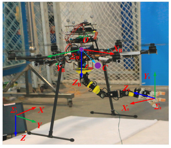
Figure 1.
Frames in aerial manipulator system.
The absolute position of the hex-rotor with respect to ΣI is denoted by , and the attitude is described by the Z−Y−X Euler angles denoted by , where φ, θ and ψ are roll, pitch and yaw angle, respectively. The rotation matrix from ΣB to ΣI is denoted by . The detail of is as follow:
where c and s denote trigonometric functions cos( ) and sin( ), respectively.
The absolute position of the end-effector with respect to ΣI is denoted by . The absolute attitude of the end-effector with respect to ΣI is denoted by . The attitude of the end-effector relative to hex-rotor with respect to ΣB is denoted by . As in Equation (1), determines the rotation matrix from ΣE to ΣI, denoted by , and determines the rotation matrix from ΣE to ΣB, denoted by . They have relation with the position and attitude of the hex-rotor as follows:
where is position of the end-effector relative to hex-rotor with respect to ΣB. For and , they can be got through forward kinematics of the manipulator with the joint angle [26]. denotes the absolute velocity of the hex-rotor with respect to ΣI. denotes the absolute angular velocity of hex-rotor with respect to ΣB. They have a relationship with and as follows:
where .
The absolute velocity and angular velocity of end-effector with respect to ΣI are denoted by and , respectively. They have a relationship with and as follows:
where and are the velocity and angular velocity of the end-effector relative to the UAV body fixed frame with respect to ΣB. and can be got through velocity kinematics of the robotic arm, as follow:
where q is the joint angle vector of the robotic arm. is joint velocity vector of the robotic arm. is the Jacobian matrix of the robotic arm and it is a function of q.
2.2. Dynamic of the UAV
The aerial manipulator can be taken as a special aerial platform whose mass distribution could be changed due to the movement of the robotic arm. The disturbance that the manipulator imposes on the hex-rotor can be partially represented by the motion of the CoM offset. Thus, the CoM offset in the UAV’s dynamic model can partially reflect influence of the robotic arm, as in a previous work [27]. The dynamics of the hex-rotor with the CoM offset, , is expressed as follows [28]:
where is the total mass of the aerial manipulator system. g is the gravity acceleration. , and are the unit vectors with three dimensions. is the inertia matrix of the hex-rotor. Ft and τ are the thrust and torque acting on the hex-rotor, respectively, and they are generated by the rotors of the hex-rotor. is CoM offset with respect to ΣB. is a function of the q that is joint angle vector of the robotic arm. Thus, based on the kinematics of the robotic arm [26], can be calculated through the measurement of the joint angles. and are force and torque disturbance, respectively, and they include wind disturbance and disturbance of the robotic arm excepting CoM offset terms.
Remark I: The CoM offset terms in the hex-rotor dynamics, Equations (6) and (7), contain the partial static disturbance of the robotic arm, and don’t contain the disturbance caused by the inertia matrix changing, and don’t contain the dynamic disturbance that is caused by joint velocity and acceleration of the robotic arm. We consider other parts of the disturbance in and .
As we know, the driving thrust and torque of the hex-rotor come from the aerodynamic force of high speed rotating rotors. The hex-rotor totally has six rotors, and serial number and rotation direction of the rotors are shown in Figure 2. The angular velocity of rotor i is denoted by (i = 1; 2; …; 6). Thrust and torque are related to the rotor speed of the rotors as follow:
where is thrust coefficient. is torque coefficient. d is the distance from center of rotor to the geometrical center of the hex-rotor. M is the mixer matrix of the hex-tor and is the vector of square of rotor speed.
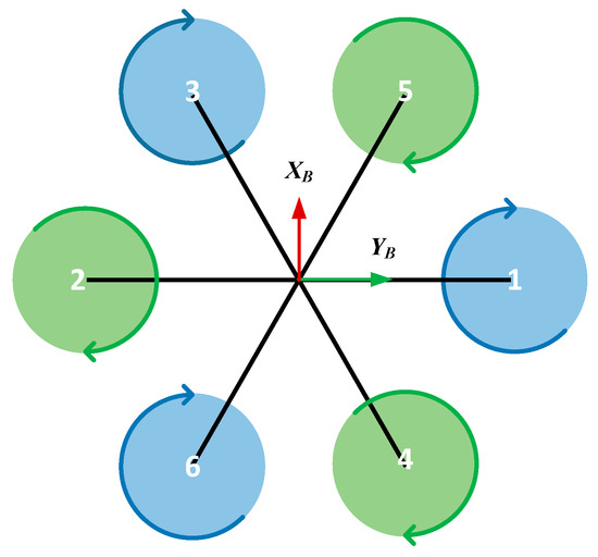
Figure 2.
Illustration of hex-rotor.
3. System Control
3.1. Hex-rotor Control
The control structure of the aerial manipulator is shown in Figure 3. The hex-rotor controller is composed of a H∞ controller and acceleration feedback enhance term. The controller is based on a hierarchical inner-outer loop structure, in which the inner loop is the attitude control loop and the outer loop is the position control loop [29]. The H∞ controller is designed to ensure the BIBO stability of the hex-rotor. The acceleration feedback enhance term is used to compensate for wind disturbance, to improve control performance.
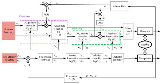
Figure 3.
Control structure of the aerial manipulator system.
3.1.1. Translational and Rotational Dynamic Decoupling
The system dynamic models in Equations (6) and (7) are the translational dynamic and rotational dynamic, respectively. In the hierarchical inner-outer loop control structure, the UAV is seen as a cascade system composed of two subsystems, that is, the translational dynamic subsystem and rotational dynamic subsystem, respectively. From Equation (6), we can see that the translational dynamic couples with the rotational dynamic through the rotation matrix . In order to decouple them, a virtual control input, , is introduced [29], and it is defined as follows:
where is the rotation matrix determined by the desired attitude angle, , which is needed in the position control loop. Substituting Equation (9) into Equation (6), the translational dynamic of the hex-rotor can be expressed as follows:
where is the attitude error defined as . is the interconnection term between the translational and rotational dynamic after decoupled by the virtual input . This virtual input is given by the H∞ position controller, which will be presented in the next subsection. Then, in order to actuate the outer loop actually, we need to translate the virtual input into the thrust and desired attitude angle, which can be tracked fast enough in the attitude control loop [29]. We define the virtual input vector as . Combining Equation (1) and Equation (9), we get the thrust, desired roll angle and desired pitch angle as follows:
Linearization of the rotational dynamic is essential to design the H∞ controller. Based on the feedback linearization theory of the MIMO (Multiple Input Multiple Output) system [30], the rotational dynamic in Equation (7) is feedback linearizable at through the following equation:
where is the virtual input of the linearized system, and it is given by the H∞ attitude controller. Thus, after decoupling and linearizing, the system dynamic will be as follows:
3.1.2. H∞ Controller
The new system in Equation (14) becomes a linear system including the interconnection term and disturbance. For a system without disturbance, a linear controller can guarantee the asymptotic stability [29]. In this section, the design of a robust H∞ control to ensure the BIBO stability of the system with the interconnection term and disturbance is described. The robust H∞ controller was designed under the assumption that the external disturbance is bounded. Although several works show such an assumption is restrictive [31,32], such an assumption can be taken in practice for an aerial manipulator system, because the manipulator always works as a fixed base manipulator in real aerial manipulation applications. So, we consider it as bound disturbance in this paper. There exist works in the literature [31,33] that tackle uncertainty in a better way, which can be considered in the future.
Remark II: In practice, the unmodeled part disturbance of the manipulator, and , can be seen as bound disturbance in the working states.
For the hex-rotor, the position and yaw angle are usually chosen as system outputs. We use to denote the desired position. The system state error is denoted by , , and . Combining Equation (3) with Equation (14), the error dynamic of the system can be written as the following equation:
where , , , , , , , , .
For the interconnection term , we have following theorem.
Theorem 1.
Forin the system (15), there exists a constant, such that
where.
The proof of Theorem 1 is given in the Appendix A.
Theorem 2.
If a feedback controllerand a positive definite symmetric matrix P can be found satisfying the following inequality:
where, λ is a positive constant. Then, system in Equation (15) will be finite gain L2-stable from disturbances Δ to outputs y and the L2 gain is less than or equal to γ.
Proof.
The Lyapunov function of the closed-loop system is defined as follow:
Thus we have,
Combining Equation (16) with Equation (19), yields,
If Equation (17) is satisfied, we have,
This means that, for any T>0,
That is,
This means that the system is finite gain L2-stable from disturbance Δ to outputs y and the L2 gain is less than or equal to γ.
The gain matrix K can be got through the following LMI:
where X is a positive definite matrix. Once W and X are obtained, the control law is as follow:
Then the closed-loop system will become asymptotically stable and the H∞ norm from disturbance ∆ to output y is less than or equal to γ. So, the virtual inputs, and , are as follows:
Combining Equation (12) and Equation (13), the Ft and τ needed for the hex-rotor can be found. It is the H∞ controller of the hex-rotor that can ensure system BIBO stability and compensate partial disturbance of the robotic arm. □
3.2. Acceleration Feedback Enhanced
When the aerial manipulator works in strong wind, although the H∞ controller can ensure system stability with proper parameters, the control performance will be seriously reduced by the wind disturbance. To attenuate disturbance of wind and unmolded part of the robotic arm, the acceleration feedback enhanced method is used in the H∞ controller. Firstly, we used the Kalman Filter to estimate the acceleration and angular acceleration of the hex-rotor, and they are denoted by and , respectively [34]. As we know, velocity and acceleration can form a first order linear system:
where, is true velocity at time . ∆t is the time interval, and is the process noise which is assumed to be zero mean multivariate normal distribution with covariance , and . is the measurement velocity at time . is the observation noise, assumed to be zero mean Gaussian white noise with covariance , and . The critical elements for the Kalman Filter are the covariance of process and observation noise. With the measurement velocity and system Equation (27), the acceleration can be estimated by Kalman Filter. For the angular acceleration, it is similar to the linear acceleration.
Based on Equation (14), the total disturbance in the translational and rotational dynamic can be estimated as follows:
where and are the estimated disturbance in the translational and rotational dynamic, respectively
Usually, the estimated acceleration includes high frequency noise because of the vibration, so that estimated disturbance, , cannot be used directly in the controller. The wind disturbance tends to lower frequency. As shown in Figure 3, to eliminate high frequency noise, is combined with a low pass filter as follow:
where is a second order low frequency pass filter. is an acceleration feedback enhanced term, and can be added into the controller of Equation (12) and (13) to compensate wind disturbance.
3.3. Manipulator Control
The manipulator controller structure is shown in Figure 3. The position controller of the end-effector is a PID (Proportion Integral Derivative) controller, so that we can get the desired velocity of the end-effector in the frame ΣI, and they are denoted by and , respectively. The velocity control of the end-effector is realized in the frame ΣB. The desired velocities of the end-effector in the frame ΣB are denoted by and , respectively. To get and , inverse velocity kinematics of the aerial manipulator system is used in the manipulator controller. Through inversing Equation (4), and can be found as follows:
The theme of velocity control of a manipulator is to find the right joint velocity that can generate the desired velocity of the manipulator end-effector. After getting the desired joint velocity, denoted by , the actuators have a low level controller, which can track the desired joint velocity with enough accuracy. The velocity control of the redundant manipulator has a framework that is introduced in a previous work [35], which can minimize , where W is a symmetric positive-definite weighting matrix and is a scalar. This frame can be described as follow:
where . is a matrix whose columns are a spanning set of the null space of . That is . is the gradient of f(q), which is a function of the joint angle vector.
4. Experiments and Results
In order to validate the wind disturbance rejection performance of the acceleration feedback enhanced H∞ controller presented in Section 3, the experiments of aerial grasping of a target object in the wind are conducted. The experimental platform and results will be introduced in this section.
4.1. Experimental Platform
The experimental platform is shown in Figure 4. The axial flow fan is used to generate wind disturbance. The anemometer is used to measure the wind speed. The aerial manipulator system mainly consists of a hex-rotor UAV, a 7-DoF robotic arm and an under-actuated gripper. The main parameters of the aerial manipulator are listed in Table 1. The tuned propulsion system of the hex-rotor is E800 of DJI powered by a 6 cell Li-Po battery. The flight stack of the hex-rotor is an open source controller for autonomous drones named PixHawk. The robotic arm is composed of Dynamixel smart actuators. The computer used as the arm controller is Intel NUC with a core-i7 processor. The under-actuated gripper is designed based on the Yale OpenHand Project [36], with some structures and parameters changed. The experiments are conducted in the OptiTrack, an indoor motion capture system.
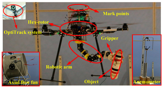
Figure 4.
Experimental platform.

Table 1.
Parameters of aerial manipulator.
The operational space of the aerial manipulator system is shown in Figure 5. The operational space Ω is a space in the front of the hex-rotor, in which the target object is away from the hex-rotor with a safe distance, and is also reachable for the robotic arm. The space is part of the space between two concentric spherical surfaces, whose center is point O (the coordinate origin ΣB.) and radiuses are lmin and lmax, respectively. The area is also limited in four planes. Its projection on the XB-O-YB and XB-O-ZB planes are shown in Figure 6. Any point T in the space will satisfy the following inequalities:
where is the position of point T relative to hex-rotor body fixed frame with respect to ΣB. Proj(.) is a function that projects a vector in the coordinate plane (X-O-Y or X-O-Z plane). α is the yaw angle range of the space Ω. βmin and βmax are the pitch angle range limit of the space Ω.
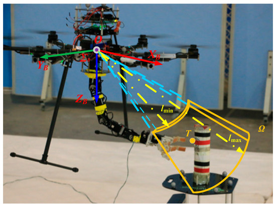
Figure 5.
Operational space of aerial manipulator.
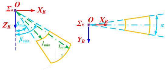
Figure 6.
Projection of the operational space Ω in the XB-O-ZB (left) and XB-O-YB (right) planes.
4.2. Aerial Grasping in the Wind
When the aerial manipulator grasps a target object, the hex-rotor is hovering at one point to keep the object in the operational space, so that the manipulator can grasp the target safely. Thus, high precision hovering is essential for the aerial manipulator to grasp a target in the wind. If the hex-rotor cannot keep the target in the operational space all the time, the target will not be reachable for the robotic arm.
The speed of wind disturbance in the experiments is shown in Figure 7a. The wind was sweeping periodically, as in Figure 7a, because the axial flow fan is switched between turn-on and turn-off to generate gusty wind disturbance. The mean and variance of the gusty wind speed were 6.54 m/s and 1.5265 m/s, respectively. The wind speed in the frequency domain is shown in Figure 7b. The main frequency of the wind disturbance was 0-0.9 Hz. Therefore, to eliminate the main part of the wind disturbance, 0.9 Hz was chosen as the cut-off frequency of the low pass filter, Q(S), in the acceleration feedback enhanced controller.
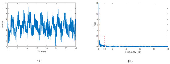
Figure 7.
The speed and frequency of the gusty wind disturbance in the experiments: (a) The speed of the gusty wind disturbance; (b) The frequency domain diagram of the of the gusty wind disturbance.
In order to validate the wind disturbance rejection performance of the acceleration feedback method, in the experiments the aerial manipulator was controlled by the robust H∞ controller without and with the acceleration feedback enhanced term. The system output control results are shown in Figure 8. The mean and variance of absolute value of control errors are shown in Figure 9. Contrasting the position and yaw error in the two experiments, we can see that the position control accuracy of the hex-rotor was improved significantly with acceleration feedback enhanced term. It means that the acceleration feedback term can reject the wind disturbance effectively.
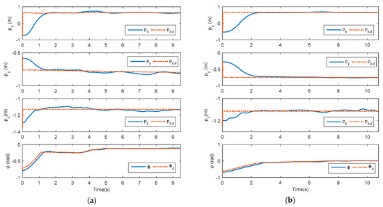
Figure 8.
The position and yaw angle of the hex-rotor: (a) The hex-rotor is controlled without the acceleration feedback enhance term; (b) The hex-rotor is controlled with the acceleration feedback enhance term.
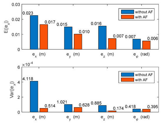
Figure 9.
The mean and variance of absolute errors of the position and yaw angle of the hex-rotor controlled with and without the acceleration feedback enhanced term.
The position of the target object in the operational space in the experiments is shown in Figure 10. It can be seen that without the acceleration feedback enhanced term, the aerial manipulator cannot keep the target object in the operational space all the time because of the weaker disturbance rejection ability. Therefore, the target becomes unreachable for the manipulator, as shown in Figure 11. As a result, the aerial grasping task fails. With the acceleration feedback enhanced term, the hex-rotor has sufficient disturbance rejection ability, and the position control accuracy of the hex-rotor is improved. Thus, the target object is kept within the operational space all the time, and the aerial grasping task is accomplished in the end, as shown in Figure 11. (The experimental video is available at the following website: https://v.youku.com/v_show/id_XNDA4NDEwODE4NA==.html?spm=a2h3j.8428770.3416059.1)
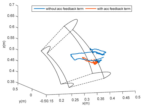
Figure 10.
Target position in the operational space when hex-rotor is controlled with and without the acceleration feedback enhanced term, respectively.
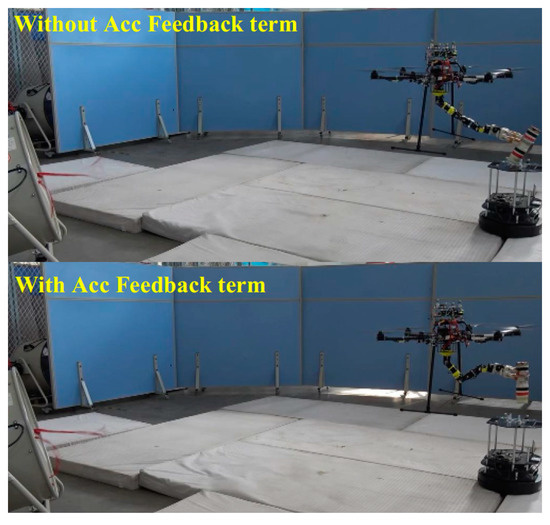
Figure 11.
Aerial grasping of target object in the wind and the hex-rotor controlled without (up) and with (down) the acceleration feedback enhanced term.
5. Conclusions
In this paper, in order to give an aerial manipulator the ability to work in the wind, we present an acceleration feedback enhanced H∞ controller. The proposed controller is based on the hierarchical inner-outer loop structure, and composed of a robust H∞ controller and the acceleration feedback enhanced term, which is used to reject the wind disturbance. This controller can improve the position control accuracy of an aerial manipulator in the wind, so that it can complete grasping tasks with wind disturbance. In future work, we will pay more attention to impedance control of the aerial manipulator to complete more complicated tasks.
Author Contributions
Conceptualization, G.Z. and Y.H.; methodology, G.Z.; software, G.Z. and B.D.; validation, G.Z. and B.D.; formal analysis, F.G. and L.Y.; investigation, G.Z.; resources, Y.H.; data curation, G.Z. and B.D.; writing—original draft preparation, G.Z., J.H. and G.L.; writing—review and editing, G.Z., J.H. and G.L.; visualization, G.Z.; supervision, Y.H., J.H. and G.L.; project administration, F.G. and L.Y.; funding acquisition, Y.H. and F.G.
Funding
This research was funded by National Key Research and Development Program of China grant number 2017YFC1405401, National Nature Sciences Foundation of China, grant number 61433016 and U1608253, and Science and Technology Planning Project of Guangdong Province, grant number 2017B010116002.
Conflicts of Interest
The authors declare no competing financial interests.
Appendix A
Proof of Theorem 1.
We define , and attitude error . Combining with Equation (1) we have,
For hx in Equation (32), replacing by and utilizing the following trigonometric functions:
we can get:
Utilizing the following inequalities into Equation (A2):
So we can get:
Similarly, we can get the property of hy and hz:
So, with Equations (A4) and (A5), we can get:
where For the hex-rotor we can assume the maximum value of the Ft is k2. So,
where, . □
References
- Bonyan Khamseh, H.; Janabi-Sharifi, F.; Abdessameud, A. Aerial manipulation—A literature survey. Robot. Auton. Syst. 2018, 107, 221–235. [Google Scholar] [CrossRef]
- Ruggiero, F.; Lippiello, V.; Ollero, A. Aerial manipulation: A literature review. IEEE Robot. Autom. Lett. 2018, 3, 1957–1964. [Google Scholar] [CrossRef]
- Mellinger, D.; Lindsey, Q.; Shomin, M.; Kumar, V. Design, modeling, estimation and control for aerial grasping and manipulation. In Proceedings of the 2011 IEEE/RSJ International Conference on Intelligent Robots and Systems, San Francisco, CA, USA, 25–30 September 2011; pp. 2668–2673. [Google Scholar]
- Pounds, P.E.I.; Bersak, D.R.; Dollar, A.M. Grasping from the air: Hovering capture and load stability. In Proceedings of the 2011 IEEE International Conference on Robotics and Automation, Shanghai, China, 9–13 May 2011; pp. 2491–2498. [Google Scholar]
- Kutia, J.R.; Stol, K.A.; Xu, W. Canopy sampling using an aerial manipulator: A preliminary study. In Proceedings of the 2015 International Conference on Unmanned Aircraft Systems (ICUAS), Denver, CO, USA, 9–12 June 2015; pp. 477–484. [Google Scholar]
- Korpela, C.; Orsag, M.; Oh, P. Towards valve turning using a dual-arm aerial manipulator. In Proceedings of the 2014 IEEE/RSJ International Conference on Intelligent Robots and Systems, Chicago, IL, USA, 14–18 September 2014; pp. 3411–3416. [Google Scholar]
- Staub, N.; Bicego, D.; Sablé, Q.; Arellano, V.; Mishra, S.; Franchi, A. Towards a flying assistant paradigm: The OTHex. In Proceedings of the 2018 IEEE International Conference on Robotics and Automation (ICRA), Brisbane, Australia, 21–25 May 2018; pp. 6997–7002. [Google Scholar]
- Zhang, G.; He, Y.; Dai, B.; Gu, F.; Yang, L.; Han, J.; Liu, G. Grasp a moving target from the air: System & control of an aerial manipulator. In Proceedings of the 2018 IEEE International Conference on Robotics and Automation (ICRA), Brisbane, Australia, 21–25 May 2018; pp. 1681–1687. [Google Scholar]
- AEROARMS. Available online: https://aeroarms-project.eu/ (accessed on 23 February 2019).
- Collaborative Aerial Workers. Available online: http://www.aeroworks2020.eu/ (accessed on 23 February 2019).
- Caccavale, F.; Giglio, G.; Muscio, G.; Pierri, F. Adaptive control for UAVs equipped with a robotic arm. IFAC Proc. Vol. 2014, 47, 11049–11054. [Google Scholar] [CrossRef]
- Lee, H.; Kim, H.J. Estimation, control, and planning for autonomous aerial transportation. IEEE Trans. Ind. Electron. 2017, 64, 3369–3379. [Google Scholar] [CrossRef]
- Pierri, F.; Muscio, G.; Caccavale, F. An adaptive hierarchical control for aerial manipulators. Robotica 2018, 36, 1527–1550. [Google Scholar] [CrossRef]
- Yang, H.; Lee, D. Dynamics and control of quadrotor with robotic manipulator. In Proceedings of the 2014 IEEE International Conference on Robotics and Automation (ICRA), Hong Kong, China, 31 May–7 June 2014; pp. 5544–5549. [Google Scholar]
- Kobilarov, M. Nonlinear trajectory control of multi-body aerial manipulators. J. Intell. Robot. Syst. 2014, 73, 679–692. [Google Scholar] [CrossRef]
- Seo, H.; Kim, S.; Kim, H.J. Aerial grasping of cylindrical object using visual servoing based on stochastic model predictive control. In Proceedings of the 2017 IEEE International Conference on Robotics and Automation (ICRA), Singapore, 29 May–3 June 2017; pp. 6362–6368. [Google Scholar]
- Garimella, G.; Kobilarov, M. Towards model-predictive control for aerial pick-and-place. In Proceedings of the 2015 IEEE International Conference on Robotics and Automation (ICRA), Seattle, WA, USA, 26–30 May 2015; pp. 4692–4697. [Google Scholar]
- Lunni, D.; Santamaria-Navarro, A.; Rossi, R.; Rocco, P.; Bascetta, L.; Andrade-Cetto, J. Nonlinear model predictive control for aerial manipulation. In Proceedings of the 2017 International Conference on Unmanned Aircraft Systems (ICUAS), Miami, FL, USA, 13–16 June 2017; pp. 87–93. [Google Scholar]
- Lippiello, V.; Ruggiero, F. Cartesian Impedance Control of a UAV with a Robotic Arm. IFAC Proc. Vol. 2012, 45, 704–709. [Google Scholar] [CrossRef]
- Huber, F.; Kondak, K.; Krieger, K.; Sommer, D.; Schwarzbach, M.; Laiacker, M.; Kossyk, I.; Parusel, S.; Haddadin, S.; Albu-Schäffer, A. First analysis and experiments in aerial manipulation using fully actuated redundant robot arm. In Proceedings of the 2013 IEEE/RSJ International Conference on Intelligent Robots and Systems, Tokyo, Japan, 3–7 November 2013; pp. 3452–3457. [Google Scholar]
- Waslander, S.; Wang, C. Wind disturbance estimation and rejection for quadrotor position control. In Proceedings of the AIAA Infotech@Aerospace Conference, Seattle, WA, USA, 6–9 April 2009; American Institute of Aeronautics and Astronautics: Reston, VA, USA, 2009. [Google Scholar]
- Shi, D.; Wu, Z.; Chou, W. Generalized extended state observer based high precision attitude control of quadrotor vehicles subject to wind disturbance. IEEE Access 2018, 6, 32349–32359. [Google Scholar] [CrossRef]
- Lee, S.J.; Kim, S.; Johansson, K.H.; Kim, H.J. Robust acceleration control of a hexarotor UAV with a disturbance observer. In Proceedings of the 2016 IEEE 55th Conference on Decision and Control (CDC), Las Vegas, NV, USA, 12–14 December 2016; pp. 4166–4171. [Google Scholar]
- Tomić, T. Evaluation of acceleration-based disturbance observation for multicopter control. In Proceedings of the 2014 European Control Conference (ECC), Strasbourg, France, 24–27 June 2014; pp. 2937–2944. [Google Scholar]
- He, Y.Q.; Han, J.D. Acceleration-feedback-enhanced robust control of an unmanned helicopter. J. Guid. Control. Dyn. 2010, 33, 1236–1250. [Google Scholar] [CrossRef]
- Spong, M.W. Robot Dynamics and Control, 1st ed.; John Wiley & Sons, Inc.: New York, NY, USA, 1989; ISBN 978-0-471-61243-8. [Google Scholar]
- Jimenez-Cano, A.; Heredia, G.; Bejar, M.; Kondak, K.; Ollero, A. Modelling and control of an aerial manipulator consisting of an autonomous helicopter equipped with a multi-link robotic arm. Proc. Inst. Mech. Eng. Part G J. Aerosp. Eng. 2016, 230, 1860–1870. [Google Scholar] [CrossRef]
- Kemper, M.; Fatikow, S. Impact of center of gravity in quadrotor helicopter controller design. IFAC Proc. Vol. 2006, 39, 157–162. [Google Scholar] [CrossRef]
- Fantoni, I.; Lozano, R.; Kendoul, F. Asymptotic stability of hierarchical inner-outer loop-based flight controllers. IFAC Proc. Vol. 2008, 41, 1741–1746. [Google Scholar] [CrossRef]
- Alberto, I. Nonlinear Control Systems; Springer Science & Business Media: Berlin/Heidelberg, Germany, 2013. [Google Scholar]
- Roy, S.; Roy, S.B.; Kar, I.N. Adaptive–robust control of euler–lagrange systems with linearly parametrizable uncertainty bound. IEEE Trans. Control. Syst. Technol. 2018, 26, 1842–1850. [Google Scholar] [CrossRef]
- Roy, S.; Roy, S.B.; Kar, I.N. A new design methodology of adaptive sliding mode control for a class of nonlinear systems with state dependent uncertainty bound. In Proceedings of the 2018 15th International Workshop on Variable Structure Systems (VSS), Graz, Austria, 9–11 July 2018; pp. 414–419. [Google Scholar]
- Roy, S.; Lee, J.; Baldi, S. A new continuous-time stability perspective of time-delay control: Introducing a state-dependent upper bound structure. IEEE Control. Syst. Lett. 2019, 3, 475–480. [Google Scholar] [CrossRef]
- Jianda, H.; Yuqing, H.; Weiliang, X. Angular acceleration estimation and feedback control: An experimental investigation. Mechatronics 2007, 17, 524–532. [Google Scholar]
- English, J.D.; Maciejewski, A.A. On the implementation of velocity control for kinematically redundant manipulators. IEEE Trans. Syst. Man Cybern. Part. Syst. Hum. 2000, 30, 233–237. [Google Scholar] [CrossRef]
- Yale OpenHand Project. Available online: https://www.eng.yale.edu/grablab/openhand/ (accessed on 12 February 2019).
© 2019 by the authors. Licensee MDPI, Basel, Switzerland. This article is an open access article distributed under the terms and conditions of the Creative Commons Attribution (CC BY) license (http://creativecommons.org/licenses/by/4.0/).