Influence of Time Delay in Signal Transmission on Synchronization between Two Coupled FitzHugh-Nagumo Neurons

Featured Application

The paper provides a new method to consider the synchronization between two neurons, which can be used to analyze other coupled oscillators.

Abstract

In this paper, the energy method is employed to analytically investigate the influence of time delay in signal transmission on synchronization between two coupled FitzHugh-Nagumo (FHN) neurons. Unlike pre-existing methods that deal with synchronization problems, our major idea is to consider the change rate of the energy of the synchronization error system, since the original system’s synchronization is equivalent to the disappearance of the energy of the error system. In rewriting the original coupled system in the corresponding energy coordinates based on the energy method, we find that the change rate of energy of the error system can be divided into two parts (periodic and non-periodic). The synchronization criterion for the original system can then be obtained by letting the non-periodic part of the change rate of the energy be less than zero. The correctness of the analysis is illustrated with numerical simulations. Our analytical results show that time delay in signal transmission has very significant effects on the synchronization between two FHN neurons. If the time delay in signal transmission is not taken into account in the two coupled FHN neurons, synchronous spikes cannot be achieved in the system for any given coupling strength. By adjusting the value of the time delay in signal transmission, the neural system can freely switch between neural rest and synchronous spikes. This means that time delay in signal transmission is crucial for the occurrence of synchronous spikes in the FHN neural system, which contributes to our understanding of the interaction between neurons. We analytically show the influence of the time delay on the synchronization between two FHN neurons, which was seldom considered by other researchers.

1. Introduction

Neural systems have received much interest over the last few years due to the great significance of technological and scientific fields. The neural system is composed of a large number of neurons, which are considered as basic units. However, a realistic neuron is too complex to be modeled using precise dynamical equations. For simplicity, the four variable Hodgkin–Huxley (HH) equation and its modified versions [1,2] are usually used to construct neural networks. The FitzHugh–Nagumo (FHN) model [3], with cubic nonlinearity is a simplified model of the HH equation as it extracts excitability of the behavior dynamics, which can exhibit hard oscillations, separatrix loops, as well as cause bifurcation of equilibria and limit cycles [4]. The FHN-like systems are of fundamental importance in the description of the qualitative nature of nerve impulse propagation and neural activity. In recent years, the FHN model was commonly used to investigate neural behavior by applying nonlinear dynamical theory [5,6,7].

On the other hand, considerable time delays are ubiquitous in all biological processes. For connected neurons, time delay occurs in the propagation of action potentials along the axon and in the transmission of signals across the synapse. The speed of signal transmission through unmyelinated axonal fibers is in the order of 1 m/s, which results in the existence of time delays of up to 80 m/s for propagation through the cortical network [8,9]. The interaction delay between the oscillators can even be as large as the oscillation period [10]. Thus, time delay is inevitable in signal transmission for real neurons. Furthermore, it has been found that time delays play an important role in the system dynamics and cannot be ignored in the modeling [11,12,13,14,15]. Coupled FHN neurons with time-delays were investigated for bifurcation [16,17,18,19]. The coupled FHN neurons had Gaussian noise and a time delay added to study the stochastic resonance phenomenon [20].

Synchronization is a common and crucial phenomenon in neural systems, which can help to understand the mutual interactions of coupled neurons and to obtain a consensus and phase locking among the corresponding states [21,22,23,24,25]. In many regions of the brain, synchronization activity has been observed and is considered as a correlate of behavior and cognition [26]. To understand information processing in the brain, complex dynamics and synchronization of oscillatory phenomena have been studied [27,28]. The synchronization conditions of coupling strength, the influence of noise and the effects of parameter mismatch have also been studied [29,30,31].

Many methods have been proposed to investigate the dynamical system synchronization and to obtain some synchronization conditions. The Lyapunov function technology is very commonly adopted to tackle synchronization problems with or without time delays. However, it is very difficult to find an appropriate Lyapunov function for nonlinear systems, especially for highly nonlinear systems with multiple delays. There is still no general approach for constructing a proper Lyapunov function. Furthermore, the synchronization conditions derived by using the Lyapunov approach are usually sufficient and highly conserved. In addition, the approach seems to be infeasible for systems with multiple components of different types [32]. For delay differential systems, the synchronization conditions based on the Lyapunov function approach are typically delay-independent, where the synchronization system often reduces to the situation system so that every solution converges asymptotically to a unique synchronous equilibrium point [33]. Pecora and Carroll [34] proposed the famous master stability function (MSF) method to discuss the local stability of the synchronization manifold. However, the stability analysis in the MSF method still requires the numerical calculation of the conditional Lyapunov exponents. This problem is also met in the matrix measure approach proposed by Chen [35]. Lu and Chen [36] analytically obtained the synchronization conditions by calculating the distance between trajectories and the synchronization manifold. Their synchronization conditions require knowledge of the synchronization trajectory, which is usually unknown before solving the system. As mentioned above, a shortcoming in the methods presented is the difficulty to analytically derive synchronization conditions for dynamical systems, especially for the delay differential systems. The influence of delay on synchronization conditions has seldom been analytically treated in previous research.

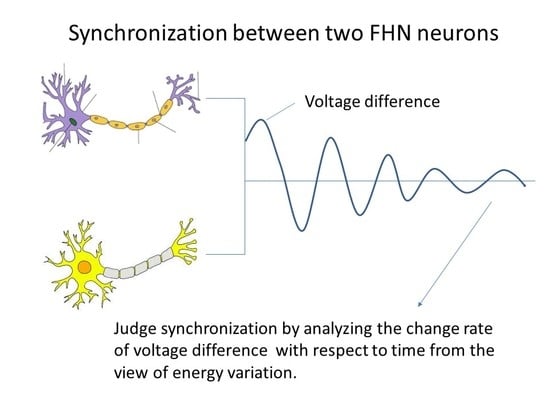
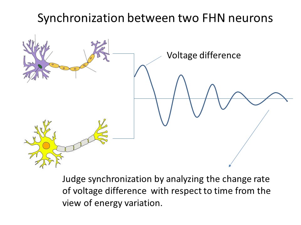
In this paper, we analytically investigate the effects of time delay in signal transmission on synchronization between two coupled FHN neurons. It is easy to understand that synchronization between two neurons will be achieved when the energy of the synchronization error system derived from the original neural system disappears. To study the change of the energy of the error system, we first rewrite the original neural system in its corresponding energy coordinates according to the energy method proposed [37]. Then, we calculate the rate of change of the energy of the error system to judge whether the energy disappears. The disappearance of energy of the error system requires for the rate of the change of the energy to be less than zero. In this way, we derive the synchronization conditions for two coupled FHN neurons without and with delay, respectively. Therefore, we can analytically estimate the influence of time delay on the synchronization conditions and study how the time delay affects the synchronous dynamics of the FHN neural system. We show that whether or not synchronization occurs between two FHN neurons, it is entirely dependent on the value of the time delay in signal transmission between two neurons. If the time delay is ignored, synchronization does not appear for any given coupling strength.

The rest of the paper is organized as follows. In Section 2, the synchronization between two coupled FHN neurons without time delay is investigated by using the energy method. In this case, a stability analysis is completed in order to prove that synchronous spikes do not occur, the correctness of which is demonstrated by numerical simulations. In Section 3, the influence of the time delay on synchronization conditions and synchronous dynamics are discussed analytically and numerically. Conclusions are drawn in Section 4.

2. Synchronization of Two Coupled FHN Neurons without Time Delay

A single FHN neuron [38] is modeled in this paper by the following equation:

$$\begin{array}{l}{\dot{u}}_1=-u_1(u_1-1)(u_1-a)-u_2,\\ {\dot{u}}_2=b(u_1-\gamma u_2).\end{array}$$

(1)

The FHN system describes the generation of the nerve impulse in a squid as well as its propagation along the giant axon. Here $u_1$ represents the potential difference at time $t$ across the membrane of the axon and $u_2$ is a recovery current caused by all ion flows. According to experiments [1], for the space clamp segment of the axon it is required that $0<a<0.5$, $b$, $\gamma >0$ in Equation (1). Furthermore, from biophysical considerations, it is rational to let $1/\gamma -(1-a+a^2)/3>0$, $(1-a+a^2)/3-b\gamma >0$.

We consider the coupled FHN neural system as:

$$\begin{array}{l}{\dot{u}}_1=-u_1(u_1-1)(u_1-a)-u_2+c(u_1-u_3),\\ {\dot{u}}_2=b(u_1-\gamma u_2),\\ {\dot{u}}_3=-u_3(u_3-1)(u_3-a)-u_4+c(u_3-u_1),\\ {\dot{u}}_4=b(u_3-\gamma u_4),\end{array}$$

(2)

where $c$ is the coupling strength. It is said that the two FHN neurons are synchronized if:

$$\underset{t\to \infty }{\lim }(u_1-u_3)=0\begin{array}{cc},& \underset{t\to \infty }{\lim }(u_2-u_4)=0\end{array}.$$

For the first and third equations in Equation (2), taking derivative with respect to time $t$ on both sides yields:

$$\begin{array}{l}{\ddot{u}}_1=[-3u_1^2+2(a+1)u_1-a+c]{\dot{u}}_1-{\dot{u}}_2-c{\dot{u}}_3,\\ {\ddot{u}}_3=[-3u_3^2+2(a+1)u_3-a+c]{\dot{u}}_3-{\dot{u}}_4-c{\dot{u}}_1.\end{array}$$

Substituting the second and forth equations in Equation (2) into the above two equations, respectively, we are able to eliminate the variables $u_2$ and $u_4$ in Equation (2), which become:

$$\begin{array}{l}{\ddot{u}}_1+(3u_1^2+{\alpha }_1{u}_1+{\alpha }_2){\dot{u}}_1+{\alpha }_3{u}_1^3+{\alpha }_4{u}_1^2+{\alpha }_5{u}_1+{\alpha }_6{u}_3+c{\dot{u}}_3=0,\\ {\ddot{u}}_3+(3u_3^2+{\alpha }_1{u}_1+{\alpha }_2){\dot{u}}_3+{\alpha }_3{u}_3^3+{\alpha }_4{u}_3^2+{\alpha }_5{u}_3+{\alpha }_6{u}_1+c{\dot{u}}_1=0,\end{array}$$

(3)

where ${\alpha }_1=-2(a+1)$, ${\alpha }_2=b\gamma +a-c$, ${\alpha }_3=b\gamma$, ${\alpha }_4=-(a+1)b\gamma$, ${\alpha }_5=b[(a-c)\gamma +1]$, ${\alpha }_6=bc\gamma$.

Therefore, we only need to consider the condition $\underset{t\to \infty }{\lim }(u_1-u_3)=0$ in system (3). By letting:

$$e_1=\frac{u_1-u_3}{2},e_2=\frac{u_1+u_3}{2},$$

Equation (3) can be written as:

$$\begin{array}{l}{\ddot{e}}_1+[3(e_1^2+e_2^2)+{\alpha }_1{e}_2+{\alpha }_2-c]{\dot{e}}_1+(6e_2+{\alpha }_1)e_1{\dot{e}}_2+{\alpha }_3{e}_1^3+(3{\alpha }_3{e}_2^2+2{\alpha }_4{e}_2+{\alpha }_5-{\alpha }_6)e_1=0\\ {\ddot{e}}_2+[3(e_1^2+e_2^2)+{\alpha }_1{e}_2+{\alpha }_2+c]{\dot{e}}_2+(6e_2+{\alpha }_1)e_1{\dot{e}}_1+{\alpha }_3{e}_2^3+(3{\alpha }_3{e}_1^2+{\alpha }_5+{\alpha }_6)e_2+{\alpha }_4(e_1^2+e_2^2)=0.\end{array}$$

(4)

Clearly, $e_1$ represents the difference between $u_1$ and $u_3$. When $e_1\to 0$, that is when $e_1$ approaches 0, Equation (2) will achieve the synchronization state. Furthermore, we use the energy method [37] to investigate the evolution tendency of $e_1$. We firstly denote four functions:

$$\begin{array}{l}{g}_1(e_1)={\alpha }_3{e}_1^3,\\ g_2(e_2)={\alpha }_3{e}_2^3+({\alpha }_5+{\alpha }_6)e_2,\\ f_1(e,\dot{e})=[3(e_1^2+e_2^2)+{\alpha }_1{e}_2+{\alpha }_2-c]{\dot{e}}_1+(6e_2+{\alpha }_1)e_1{\dot{e}}_2\\ \begin{array}{cc}& +(3{\alpha }_3{e}_2^2+2{\alpha }_4{e}_2+{\alpha }_5-{\alpha }_6)e_1\end{array},\\ f_2(e,\dot{e})=[3(e_1^2+e_2^2)+{\alpha }_1{e}_2+{\alpha }_2+c]{\dot{e}}_2+(6e_2+{\alpha }_1)e_1{\dot{e}}_1\\ \begin{array}{cc}& +3{\alpha }_3{e}_1^2{e}_2+{\alpha }_4(e_1^2+e_2^2)\end{array}.\end{array}$$

By considering the physical meanings of parameters ${\alpha }_{3,5,6}$, it is easy to check that:

$$\begin{array}{l}{e}_1{g}_1{(e_1)}_{e_1\ne 0}={\alpha }_3{e}_1^4>0,\\ e_2{g}_2{(e_2)}_{e_2\ne 0}={\alpha }_3{e}_2^4+({\alpha }_5+{\alpha }_6)e_2^2>0.\end{array}$$

On the other hand, the two variables $u_1$ and $u_3$ in system (3) represent membrane voltage difference, which are obviously bound in the real world. Correspondingly, $e_1$ and $e_2$ are bound. Therefore, the energy method [37] can be applied to Equation (4).

According to the energy method, we can observe that Equation (4) describes the movements of two oscillators. $e_1$ and $e_2$ represent the positions of two oscillators, respectively. $e_1\to 0$ means that the mechanical energy of the corresponding oscillator finally disappears. This implies that we can judge whether $e_1\to 0$ by analyzing the variation of mechanical energy of the oscillator. We denote the potential and mechanical energy of two oscillators in Equation (4) by $V_i(e_i)$ and $E_i(e_i,{\dot{e}}_i)$, $i=1,2,$ respectively, which can be written as:

$$\begin{array}{l}{V}_1(e_1)={\displaystyle {\int }_0^{e_1}({\alpha }_3{e}_1^3)}d{e}_1=\frac{1}{4}{\alpha }_3{e}_1^4,\\ V_2(e_2)={\displaystyle {\int }_0^{e_2}[{\alpha }_3{e}_2^3+({\alpha }_5+{\alpha }_6)e_2]}d{e}_2=\frac{1}{4}{\alpha }_3{e}_2^4+\frac{1}{2}({\alpha }_5+{\alpha }_6)e_2^2,\\ E_i(e_i,{\dot{e}}_i)=V_i(e_i)+\frac{1}{2}{\dot{e}}_i,i=1,2.\end{array}$$

Since $V_i(e_i)$, $i=1$, $2$, are even functions, the energy coordinate system corresponding to Equation (4) is obtained by the following transformation:

$$\begin{array}{l}{e}_i=a_i\cos ({\theta }_i),(i=1,2),\\ {\dot{e}}_1=-\sqrt{2(V_1(a_1)-V_1(a_1\cos ({\theta }_1)))}=\pm \frac{a_1^2\sqrt{{\alpha }_3}}{4}\sqrt{5-\cos (4{\theta }_1)-4\cos (2{\theta }_1)},\\ {\dot{e}}_2=-\sqrt{2(V_2(a_2)-V_2(a_2\cos ({\theta }_2)))}\\ =\pm \frac{a_2}{4}\sqrt{5{\alpha }_3{a}_2^2+8({\alpha }_5+{\alpha }_6)-{\alpha }_3{a}_2^2\cos (4{\theta }_2)-4[{\alpha }_3{a}_2^2+2({\alpha }_5+{\alpha }_6)]\cos (2{\theta }_2)}.\end{array}$$

(5)

Neglecting the terms higher than second-order, the last two equations in Equation (5) can be written approximately as:

$$\begin{array}{l}{\dot{e}}_1=-A_1(1-\frac{1}{10}\cos (4{\theta }_1)-\frac{2}{5}\cos (2{\theta }_1)),\\ {\dot{e}}_2=-A_2(1-A_3\cos (4{\theta }_2)-A_4\cos (2{\theta }_2)),\end{array}$$

(6)

where

$$\begin{array}{l}{A}_1=\frac{\sqrt{5{\alpha }_3}{a}_1^2}{4}>0,A_2=\frac{\sqrt{5{\alpha }_3{a}_2^2+8({\alpha }_5+{\alpha }_6)}{a}_2}{4}>0,\\ 0<A_3=\frac{{\alpha }_3{a}_2^2}{2(5{\alpha }_3{a}_2^2+8({\alpha }_5+{\alpha }_6))}<\frac{1}{2},0<A_4=\frac{2({\alpha }_3{a}_2^2+2({\alpha }_5+{\alpha }_6))}{5{\alpha }_3{a}_2^2+8({\alpha }_5+{\alpha }_6)}<\frac{1}{2}.\end{array}$$

From Equations (4) and (5), we have:

$$\begin{array}{l}\frac{d{E}_1}{dt}=-f_1(e,\dot{e}){\dot{e}}_1=B_1+B_2\cos ({\theta }_1)+B_3\cos (2{\theta }_1)+B_4\cos ({\theta }_2)\\ +B_5\cos (2{\theta }_2)+B_6\cos ({\theta }_1-{\theta }_2)+B_7\cos (2{\theta }_1-2{\theta }_2)+H({\theta }_1,{\theta }_2),\end{array}$$

(7)

where

$$\begin{array}{l}{B}_1=(-\frac{651a_2^2}{400}-\frac{423a_1^2}{400}+\frac{217c}{200}-\frac{217{\alpha }_2}{200})A_1^2,\\ B_2=\frac{2}{5}(3{\alpha }_3{a}_2^2-2A_2{\alpha }_1-2{\alpha }_6+2{\alpha }_5)a_1{A}_1,\\ B_3=(-\frac{19c}{25}+\frac{19{\alpha }_2}{25}-\frac{159a_1^2}{400}+\frac{57a_2^2}{50})A_1^2,\\ B_4=-\frac{217}{200}{A}_1^2{\alpha }_1{a}_2,B_5=-\frac{651}{400}{A}_1^2{a}_2^2,\\ B_6=\frac{2}{5}(2{\alpha }_4-6A_2+3A_2{A}_4)a_2{a}_1{A}_1,B_7=\frac{57}{100}{A}_1^2{a}_2^2,\end{array}$$

and $H({\theta }_1$,${\theta }_2)$ represents the rest of the periodic functions of ${\theta }_1$,${}_2$. Obviously, $e_1\to 0$ holds when $E_1\to 0$. To make $E_1\to 0$, a non-periodic term in $d{E}_1/dt$, it should be less than zero, which means $B_1<0$ holds. Since ${\alpha }_i^2\ge 0$, $i=1$, $2$, $c-{\alpha }_2<0$, it leads to the synchronization condition:

$$c<\frac{1}{2}(a+b\gamma )<\frac{1}{6}{(1+a)}^2.$$

(8)

Next, we prove that synchronous spikes do not occur in Equation (2) under Equation (8) by analyzing the stability of the origin of Equation (2). Linearizing Equation (2) around its origin yields:

$$\frac{dU}{dt}=DU,$$

(9)

in which $U=[u_1$,$u_2$,$u_3$,$u_4{]}^T$ and:

$$D=\left[\begin{array}{cc}{D}_1& D_2\\ D_2& D_1\end{array}\right],$$

where

$$D_1=\left[\begin{array}{cc}c-a& -1\\ b& -b\gamma \end{array}\right],D_2=\left[\begin{array}{cc}-c& 0\\ 0& 0\end{array}\right].$$

(10)

The matrix $D$ can be diagonalized as:

$$\left[\begin{array}{cc}{D}_1& O\\ O& D_3\end{array}\right],$$

where $O$ is a $2\times 2$ zero matrix and $D_3=D_1-D_2{D}_1^{-1}{D}_2$. The eigenvalues of matrix $D$ consist of eigenvalues of matrixes $D_1$ and $D_3$. All eigenvalues of matrix $D$ have negative real parts if and only if:

$$\begin{array}{l}c<a+b\gamma <\frac{{(1+a)}^2}{3},c<a+\frac{1}{\gamma }<\frac{{(1+a)}^2}{3},\\ \frac{(a\gamma +1)(b\gamma +a)-c(b{\gamma }^2+2a\gamma +1)}{(a-c)\gamma +1}>0,\\ \frac{b(a\gamma +1)[(a-2c)\gamma +1]}{(a-c)\gamma +1}>0.\end{array}$$

(11)

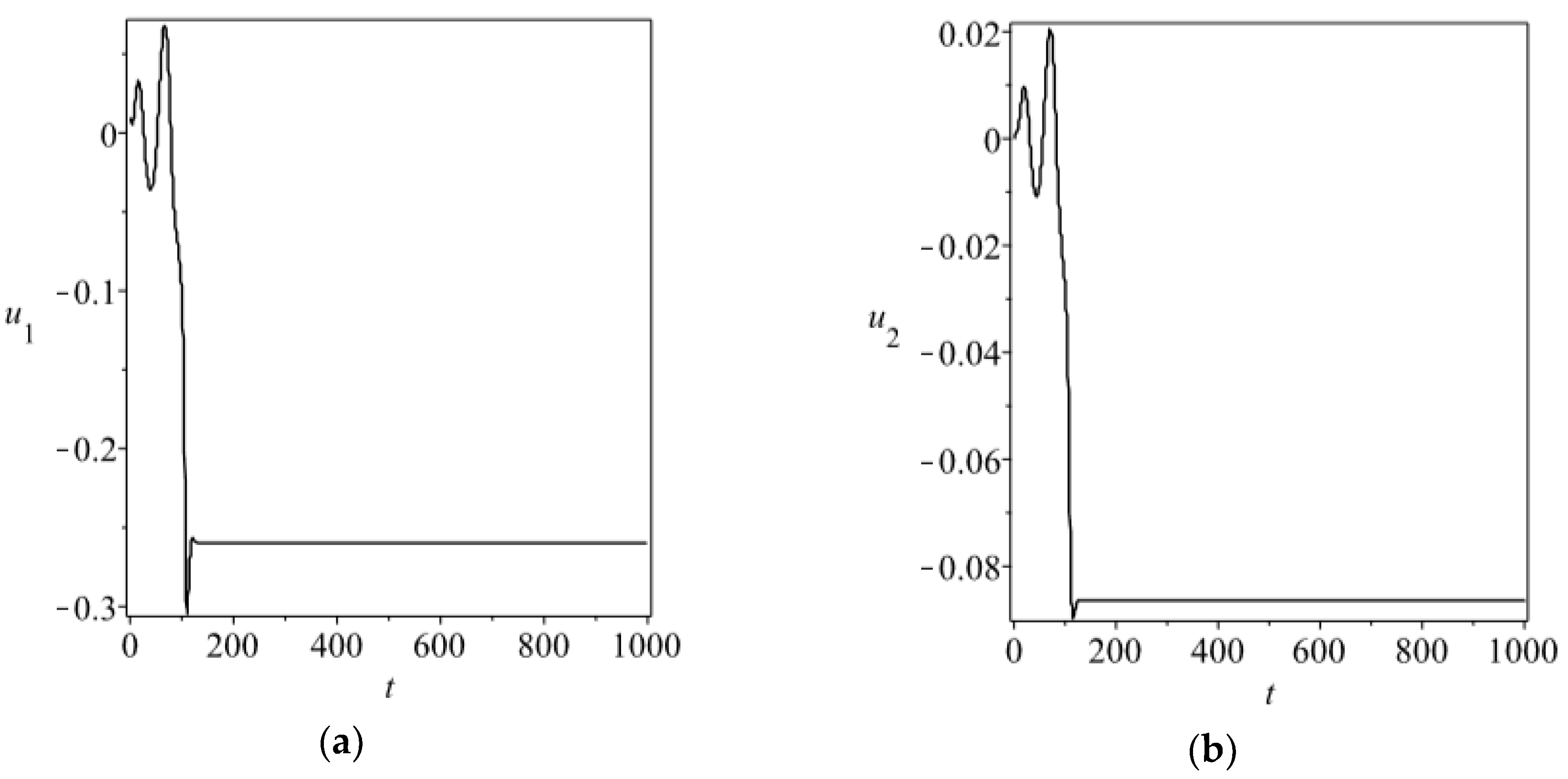
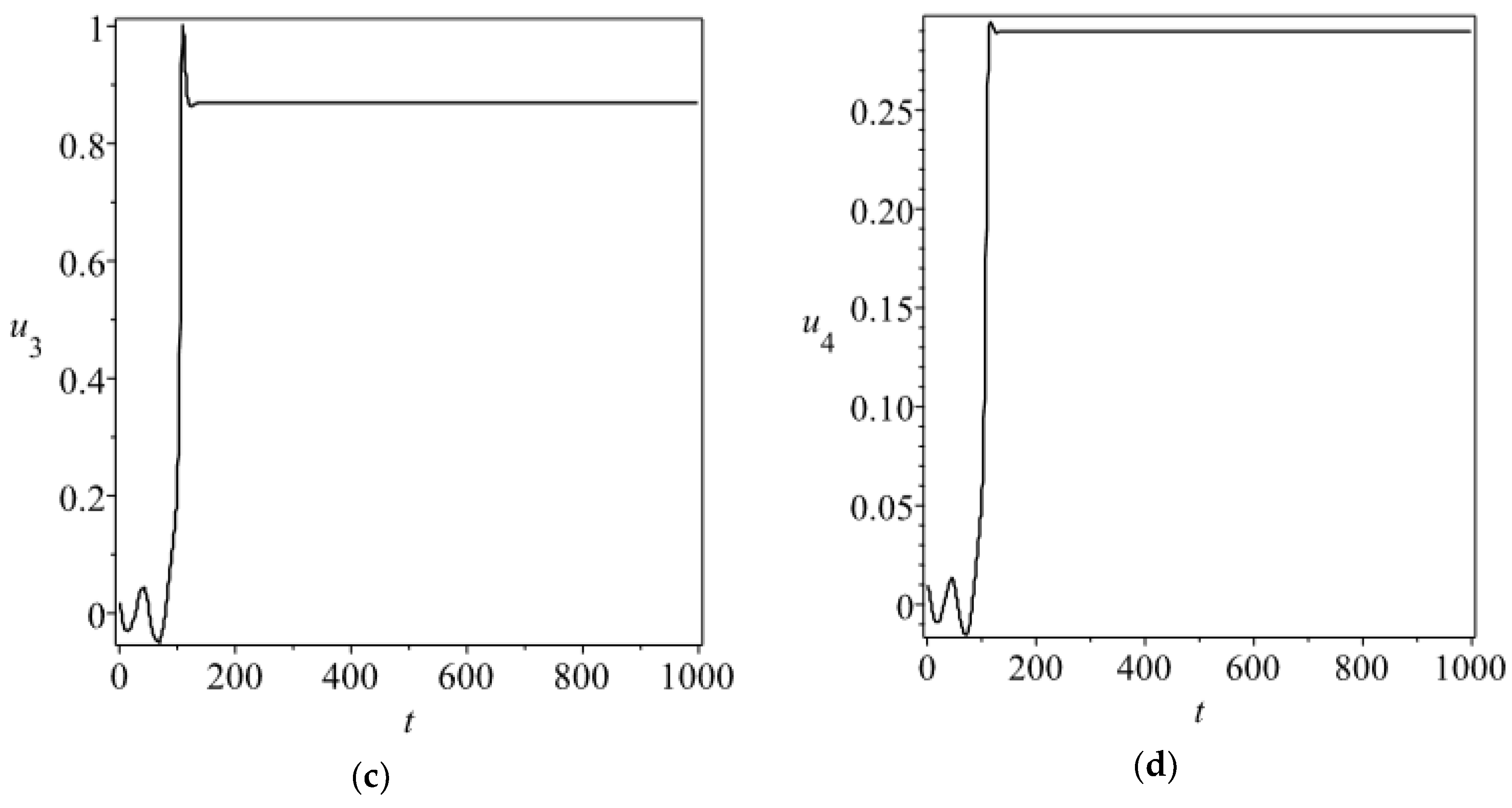
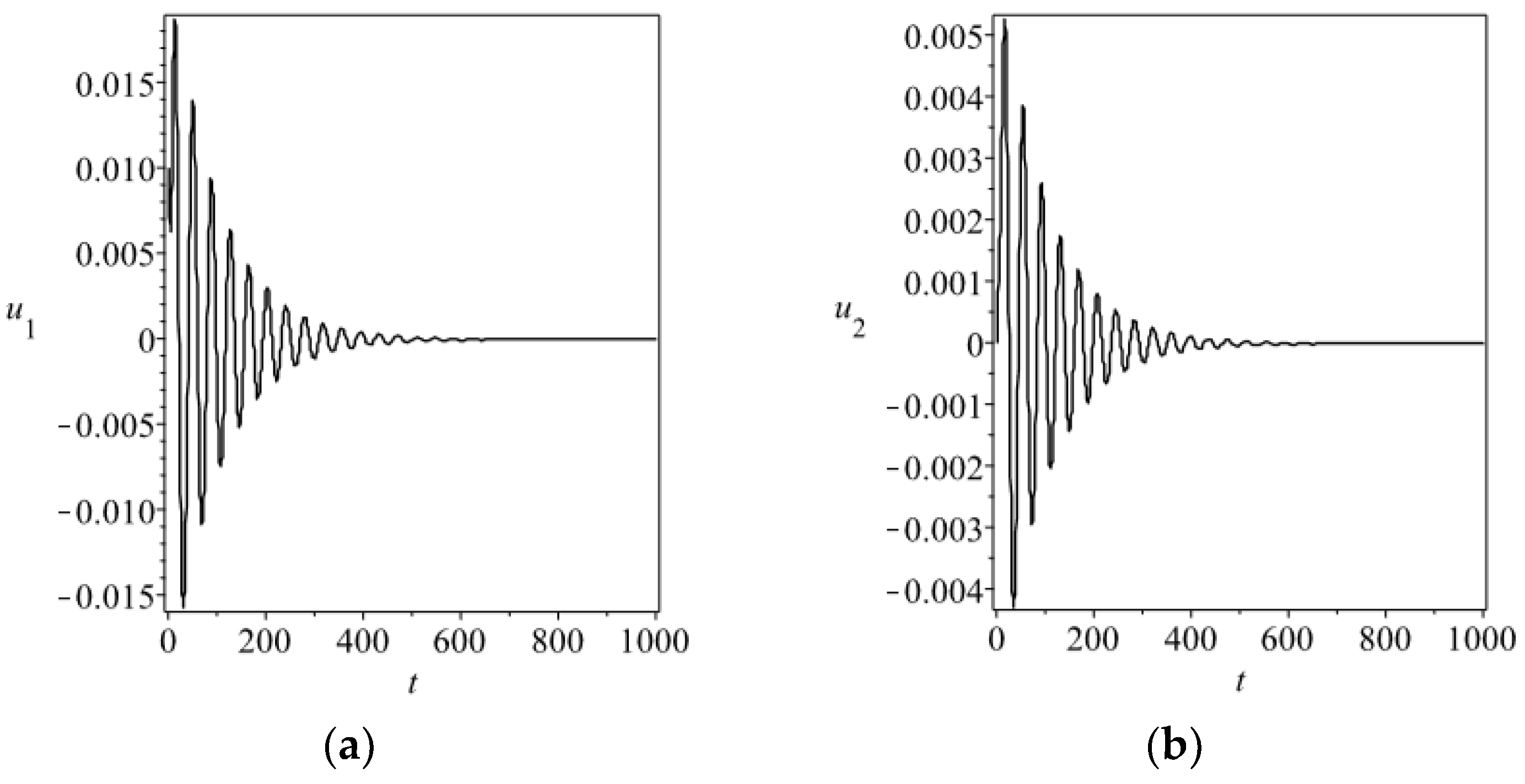
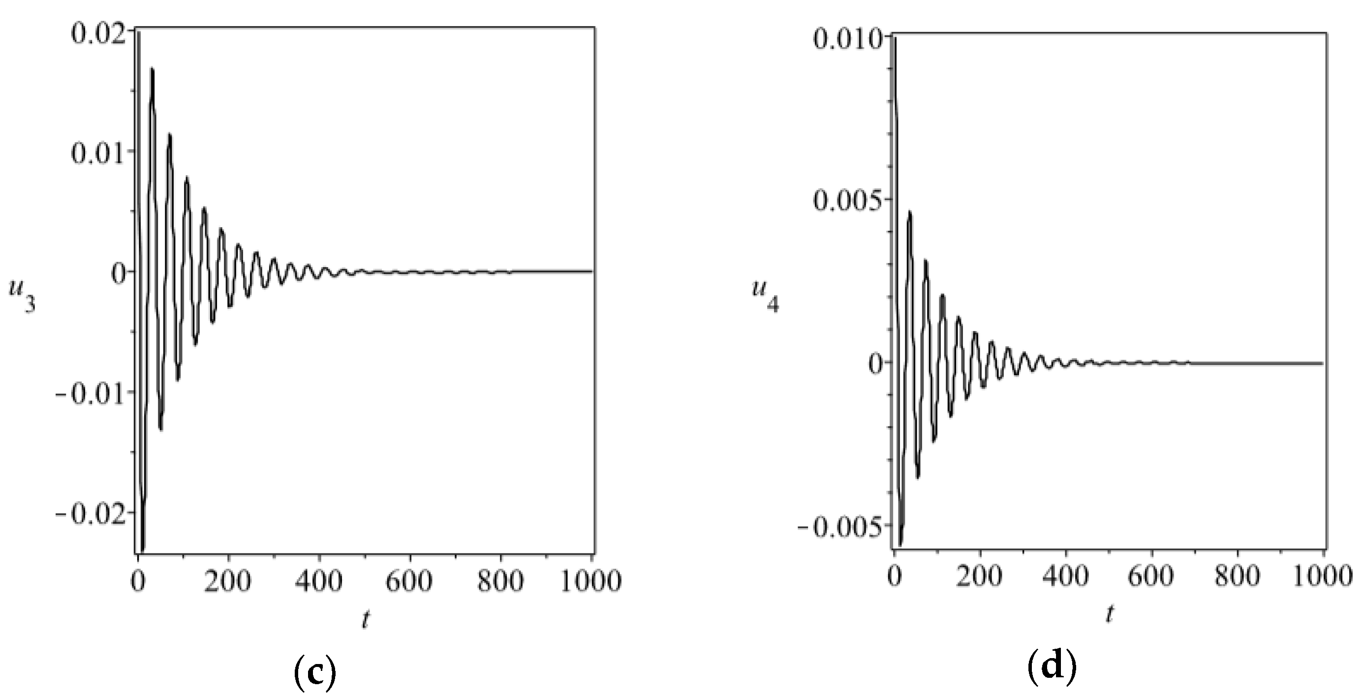
Recalling the parameter ranges defined in Equation (1), it is easy to check that all inequations in (11) hold if Equation (8) is satisfied. Therefore, the origin of Equation (2) is asymptotically stable, corresponding to the neural rest, if Equation (8) holds. This means that for any given coupling, strength $c$ synchronous spikes in Equation (1) do not occur. To demonstrate the validity of the synchronization Equation (8), we carry out some numerical simulations for Equation (2) with $a=0.1$, $b=0.08$, $\gamma =3$. The initial conditions are given by $u_1(0)=0.01$, $u_2(0)=0$, $u_3(0)=0.02$, $u_4(0)=0.01$. From Equation (8), the synchronization condition by the energy method can be written as $c<0.17$. We separately take $c=0.16$ and $c=0.18$ to carry out the numerical simulations for Equation (2), the results of which are illustrated in Figure 1 and Figure 2, respectively. Numerical simulations demonstrate the correctness of the theoretical analysis in this section. Moreover, our criterion obtained by calculating the rate of change of the energy of the error system is necessary and sufficient.

Remark 1.

In this section, we employ the energy method to analyze the synchronization between two coupled FHN neurons without time delay in signal transmission (Equation (2)). By considering the change rate of energy difference between the two neurons, we analytically derive the synchronization condition in the case of no time delay. The stability analysis for Equation (2) shows that if the time delay of signal transmission is ignored, the two neurons can only maintain neural rest when synchronization is achieved between them.

3. Two Coupled FHN Neural Systems with Time Delay

In this section, in order to consider the effects of time delay in signal transmission between two neurons, we modify Equation (2) into:

$$\begin{array}{l}{\dot{u}}_1=-u_1(u_1-1)(u_1-a)-u_2+c(u_1-u_3(t-{\tau }_1)),\\ {\dot{u}}_2=b(u_1-\gamma u_2),\\ {\dot{u}}_3=-u_3(u_3-1)(u_3-a)-u_4+c(u_3-u_1(t-{\tau }_2)),\\ {\dot{u}}_4=b(u_3-\gamma u_4),\end{array}$$

(12)

where ${\tau }_1({\tau }_2)$ represents the time delay in signal transmission from $u_3(u_1)$ to $u_1(u_3)$ and other parameters remain the same as that in Equation (2). In this paper, we place emphasis on presenting the influence of time delay in signal transmission between two neurons on synchronization conditions. We take ${\tau }_1={\tau }_2=\tau$ in Equation (12) to simplify the synchronization analysis. Similar to that of Equation (2), synchronization in Equation (12) is said to be achieved if:

$$\underset{t\to \infty }{\lim }(u_1-u_3)=0\begin{array}{cc},& \underset{t\to \infty }{\lim }(u_2-u_4)=0\end{array}.$$

Substituting:

$$e_1=\frac{u_1-u_3}{2},e_2=\frac{u_1+u_3}{2},e_3=\frac{u_2-u_4}{2},e_4=\frac{u_2+u_4}{2},$$

into Equation (12) leads to:

$$\begin{array}{l}{\dot{e}}_1=-e_1^3+[-3e_2^2+2(a+1)e_2+c-a]e_1+c{e}_1(t-\tau )-e_3,\\ {\dot{e}}_3=b(e_1-\gamma e_3),\\ {\dot{e}}_2=-e_2^3+(1+a)(e_1^2+e_2^2)-(3e_1^2+a-c)e_2-c{e}_2(t-\tau )-e_4,\\ {\dot{e}}_4=b(e_2-\gamma e_4).\end{array}$$

(13)

By eliminating $e_3$ and $e_4$, Equation (13) becomes:

$$\begin{array}{l}{\ddot{e}}_1+[3(e_1^2+e_2^2)+{\alpha }_1{e}_2+{\alpha }_2]{\dot{e}}_1+(6e_2+{\alpha }_1)e_1{\dot{e}}_2+{\alpha }_3{e}_1^3\\ \begin{array}{ccc}& & \end{array}+(3{\alpha }_3{e}_2^2+2{\alpha }_4{e}_2+{\alpha }_5)e_1-{\alpha }_6{e}_1(t-\tau )-c{\dot{e}}_1(t-\tau )=0,\\ {\ddot{e}}_2+[3(e_1^2+e_2^2)+{\alpha }_1{e}_2+{\alpha }_2]{\dot{e}}_2+(6e_2+{\alpha }_1)e_1{\dot{e}}_2+{\alpha }_3{e}_2^3\\ \begin{array}{ccc}& & \end{array}+(3{\alpha }_3{e}_1^2+{\alpha }_5)e_2+{\alpha }_4(e_1^2+e_2^2)+{\alpha }_6{e}_2(t-\tau )+c{\dot{e}}_2(t-\tau )=0,\end{array}$$

(14)

where ${\alpha }_{1,2,3,4,5,6}$, have been defined in Equation (3). We successfully applied the energy method to calculate periodic solutions of a delay differential equation [39], which involved the computations of the mechanical energy of oscillators. This illustrated that although the solution space of a delay differential system has infinite dimensions, approximate calculations of mechanical energy of oscillators are still feasible based on the energy method. Thus, we can use the energy method to analyze the mechanical energy variation of $e_1$ in Equation (14). To this end, we redefine the following functions:

$$\begin{array}{cc}\hfill g_1\left(e_1\right)={\alpha }_3{e}_1^3,g_2\left(e_2\right)& ={\alpha }_3{e}_2^3,\hfill \\ \hfill f_1(e,\dot{e},e(t-\tau ),\dot{e}(t-\tau ))& =[3(e_1^2+e_2^2)+{\alpha }_1{e}_2+{\alpha }_2]{\dot{e}}_1+(6e_2+{\alpha }_1)e_1{\dot{e}}_2\hfill \\ & +(3{\alpha }_3{e}_2^2+2{\alpha }_4{e}_2+{\alpha }_5)e_1-{\alpha }_6{e}_1(t-\tau )-c{\dot{e}}_1(t-\tau ),\hfill \\ \hfill f_2(e,\dot{e},e(t-\tau ),\dot{e}(t-\tau ))& =[3(e_1^2+e_2^2)+{\alpha }_1{e}_2+{\alpha }_2]{\dot{e}}_2+(6e_2+{\alpha }_1)e_1{\dot{e}}_1\hfill \\ & +(3{\alpha }_3{e}_1^2+{\alpha }_5)e_1+{\alpha }_4(e_1^2+e_2^2)+{\alpha }_6{e}_2(t-\tau )+c{\dot{e}}_2(t-\tau ).\hfill \end{array}$$

The potential and mechanical energy of Equation (14) can be expressed by:

$$\begin{array}{l}{V}_1(e_1)={\displaystyle {\int }_0^{e_1}({\alpha }_3)}{e}_1^{3}d{e}_1=\frac{1}{4}{\alpha }_3{e}_1^4,\\ V_2(e_2)={\displaystyle {\int }_0^{e_2}({\alpha }_3)}{e}_2^{3}d{e}_2=\frac{1}{4}{\alpha }_3{e}_2^4,\\ E(e,\dot{e})=V(e)+\frac{1}{2}\dot{e}.\end{array}$$

We define the transformation between Equation (14) and its energy coordinate $(E$,$\theta )$ as:

$$\begin{array}{l}{e}_i=a_i\cos ({\theta }_i),i=1,2,\\ {\dot{e}}_1=-C_1(1-\frac{1}{10}\cos (4{\theta }_1)-\frac{2}{5}\cos (2{\theta }_1)),\\ {\dot{e}}_2=-C_2(1-\frac{1}{10}\cos (4{\theta }_2)-\frac{2}{5}\cos (2{\theta }_2)),\end{array}$$

(15)

where

$$C_1=\frac{\sqrt{5{\alpha }_3}{a}_1^2}{4},C_2=\frac{\sqrt{5{\alpha }_3}{a}_2^2}{4},$$

(16)

Employing the energy method, we have:

$$\begin{array}{l}\frac{d{E}_1}{dt}=-f_1(e_1,{\dot{e}}_1,e_1(t-\tau ),{\dot{e}}_1(t-\tau )){\dot{e}}_1\\ =[(3(e_1^2+e_2^2)+{\alpha }_1{e}_2+{\alpha }_2){\dot{e}}_1+(6e_2+{\alpha }_1)e_1{\dot{e}}_2\\ +(3{\alpha }_3{e}_2^2+2{\alpha }_4{e}_2+{\alpha }_5)e_1-{\alpha }_6{e}_1(t-\tau )-c{\dot{e}}_1(t-\tau )]{\dot{e}}_1.\end{array}$$

(17)

Consider ${\theta }_1$ and ${\theta }_2$ have the following forms:

$$\begin{array}{l}{\theta }_1=\omega t+{\phi }_1,\\ {\theta }_2=\omega t+{\phi }_2,\end{array}$$

(18)

where $\omega \ge 0$, which will be determined later. Substituting Equations (15) and (18) into Equation (17), we have:

$$\begin{array}{l}\frac{d{E}_1}{dt}=-\frac{423a_1^2+651a_2^2}{400}+c[1+\frac{2\cos (2\omega \tau )}{25}+\frac{\cos (4\omega \tau )}{200}]-\frac{217}{200}(b\gamma +a-c)\\ +Cosineterms.\end{array}$$

(19)

Similar to that in the previous section, $E_1\to 0$ means that the non-periodic terms in Equation (19) should be less than zero. From Equation (19), the synchronization condition is given by:

$$c<\frac{217}{2{[\cos (2\omega \tau )+4]}^2+384}(a+b\gamma ).$$

(20)

$\omega$ Equation (20) can be approximately obtained from the following. The characteristic equation of Equation (12) at the origin is given by:

$${\lambda }^4+d_1{\lambda }^3+d_2{\lambda }^2+d_3\lambda +d_4+(d_5{\lambda }^2+d_6\lambda +d_7)e^{-2\lambda \tau }=0,,$$

(21)

where

$$\begin{array}{l}{d}_1=2(b\gamma +a-c),d_2=b[b{\gamma }^2+4\gamma (a-c)+2]+{(a-c)}^2,\\ d_3=2b[(a-c)\gamma +1](b\gamma +a-c),d_4=b^2{[(a-c)\gamma +1]}^2,\\ d_5=-c^2,d_6=-2b\gamma c^2,d_7=-{(bc\gamma )}^2.\end{array}$$

Substituting $\lambda =i\omega$ into Equation (21) and separating real and imaginary parts yields:

$$\begin{array}{l}{\omega }^4-d_2{\omega }^2+d_4-(d_5{\omega }^2-d_7)\cos (2\omega \tau )+d_6\omega \sin (2\omega \tau )=0,\\ d_3\omega -d_1{\omega }^3+d_6\omega \cos (2\omega \tau )+(d_5{\omega }^2-d_7)\sin (2\omega \tau )=0.\end{array}$$

(22)

Eliminating $\tau$ from Equation (22), we have:

$$p(y)=y^4+r_1{y}^3+r_2{y}^2+r_{3}y+r_4=0,$$

(23)

where

$$\begin{array}{l}y={\omega }^2,\\ r_1=d_1^2-2d_2,\\ r_2=-2d_1{d}_3+d_2^2-d_5^2+2d_4,\\ r_3=-2d_2{d}_4+d_3^2+2d_5{d}_7-d_6^2,\\ r_4=d_4^2-d_7^2.\end{array}$$

$\omega$ in Equation (20) exists and means that Equation (23) has one positive root. Assume that $\omega ={\omega }_0$ is one simple positive root of Equation (23). From Equation (22), we have:

$$\cos (2{\omega }_0\tau )=\frac{{\omega }_0^6{d}_5+(d_1{d}_6-d_2{d}_5-d_7){\omega }_0^4+(d_2{d}_7-d_3{d}_6+d_4{d}_5){\omega }_0^2-d_4{d}_7}{{\omega }_0^4{d}_5^2+(d_6^2-2d_5{d}_7){\omega }_0^2+d_7^2},,$$

(24)

In addition, by regarding $\lambda$ in Equation (21) as a function of $\tau$ and taking the derivative of both sides of Equation (21) with respect to $\tau$ yields:

$$\frac{d\lambda }{d\tau }=\frac{(2d_5{\lambda }^2+2d_6\lambda +2d_7)\lambda e^{-2\lambda \tau }}{(2{\lambda }^2\tau d_5+2\lambda \tau d_6-2\lambda d_5+2\tau d_7-d_6)e^{-2\lambda \tau }-4{\lambda }^3-3d_1{\lambda }^2-2d_2\lambda -d_3}.$$

(25)

Under Equation (11), Equation (12) with $\tau =0$ has a stable origin. At the same time if:

$$Re\left\{\frac{d\lambda }{d\tau }\right\}>0,$$

(26)

for $\omega ={\omega }_0$ and some critical value of delay determined by Equation (24), the origin of Equation (12) will lose its stability. In such a case, the coupled neural system cannot remain at neural rest. Synchronous spikes in the coupled system will occur due to an appropriate value of time delay.

The distribution of positive real roots of an algebraic equation similar to Equation (23) has been treated in other studies [40,41]. In the following, we will employ a complete discrimination system for polynomials [42,43] and the Descartes sign method to analyze the condition that Equation (23) has one or more positive real roots. We denote the Sylvester matrix of $p(y)$ and $p^{\prime }(y)$ by $Discr(p)$, where $p^{\prime }(y)$ is the derivative of $p(y)$ with respect to $y$ and denote the determinant of the submatrix of $Discr(p)$ formed by the first $2k$ rows and the first $2k$ columns by $D_k(p)$, $k=$ 1, 2, 3, 4. If the number of the sign changes in the discriminant sequence:

$$\{D_1(p),D_2(p),D_3(p),D_4(p)\}$$

(27)

is $\upsilon$, then the number of pairs of distinct conjugate imaginary roots of $p(y)$ is equal to $\upsilon$. Furthermore, if the number of nonvanishing members of the list is $l$, then the number of the distinct real roots of $p(y)$ equals to $l-2\upsilon$.

According to the procedure [42], we have:

$$\begin{array}{l}{D}_1=1,\\ D_2=3r_1^2-8r_2,\\ D_3=-4r_2^3+r_1^2{r}_2^2+2(7r_3{r}_1+8r_4)r_2-6r_1^2{r}_4-18r_3^2-3r_1^3{r}_3,\\ D_4=-27r_1^4{r}_4^2+18r_1^3{r}_2{r}_3{r}_4-4r_1^3{r}_3^3-4r_1^2{r}_2^3{r}_4+r_1^2{r}_2^2{r}_3^2\\ \begin{array}{cc}& \end{array}+144r_1^2{r}_2{r}_4^2-6r_1^2{r}_3^2{r}_4-80r_1{r}_2^2{r}_3{r}_4+18r_1{r}_2{r}_3^3+16r_2^4{r}_4\\ \begin{array}{cc}& \end{array}-4r_2^3{r}_3^2-192r_1{r}_3{r}_4^2-128r_2^2{r}_4^2+144r_2{r}_3^2{r}_4-27r_3^4+256r_4^3.\end{array}$$

(28)

We can further determine the number of positive real roots of Equation (23) based on the Descartes sign method by considering the number of the sign changes in the discriminant sequence:

$$\{1,r_1,r_2,r_3,r_4\}.$$

(29)

Then we have the following:

-

If $r_4<0$, Equation (23) has at least one positive real root.

-

If the number of sign changes in Equation (27) is zero, Equation (23) only has real roots. The number of the positive real roots equals to the number of the sign changes in Equation (29).

-

If the number of the sign changes in Equation (27) is one and the number of nonvanishing members in the sequence is 4, Equation (23) has two different real roots, the sign of which can be determined by the Descartes sign method.

-

If the number of sign changes in Equation (27) is one and the number of nonvanishing members in the sequence is 3, Equation (23) has two identical real roots, the sign of which can be determined by the Descartes sign method.

Next, we numerically show that the existence of time delay in signal transmission can make the synchronous spikes occur in Equation (12). For comparison, we keep $a=0.1$, $b=0.08$ and $\gamma =3$ in Equation (12). If $c=0.16$ or $c=0.18$, we have the following two sequences:

$$\begin{array}{l}\{D_1>0,D_2<0,D_3<0,D_4<0\},\\ \{1,r_1<0,r_2>0,r_3<0,r_4>0\}.\end{array}$$

(30)

If the number of sign changes in Equation (27) is one, then Equation (23) has two different real roots. Under such conditions, by substituting $y=-z$ into Equation (23), we have:

$$p(z)=z^4-r_1{z}^3+r_2{z}^2-r_{3}z+r_4=0.$$

(31)

Then the number of sign changes in the sequence $\{1$,$-r_1$,$r_2$,$-r_3$,$r_4\}$ is zero. Equation (31) has no positive real root, which means that Equation (23) has no negative real root. Therefore, Equation (23) with $a=0.1$, $b=0.08$, $\gamma =3$ and $c=0.16$ or $c=0.18$ has just two positive real roots. In fact, if $c=0.16$, Equation (23) has two positive real roots:

$${\omega }_1=0.173,{\omega }_2=0.307,$$

the two corresponding critical values of $\tau$ are:

$${\tau }_1=0.529+\frac{2n\pi }{0.529},n=0,1,2\dots ,$$

and:

$${\tau }_2=3.712+\frac{2n\pi }{3.712},n=0,1,2\dots ,$$

respectively. The transversality condition (Equation (26)) is satisfied only for ${\omega }_2=0.307$ and ${\tau }_2=3.712$. If $c=0.18$, Equation (23) has two positive real roots:

$${\omega }_1=0.128,{\omega }_2=0.335,$$

the two corresponding critical values of $\tau$ separately, are:

$${\tau }_1=0.516+\frac{2n\pi }{0.516},{\tau }_2=4.149+\frac{2n\pi }{4.149},n=0,1,2\dots ,$$

(32)

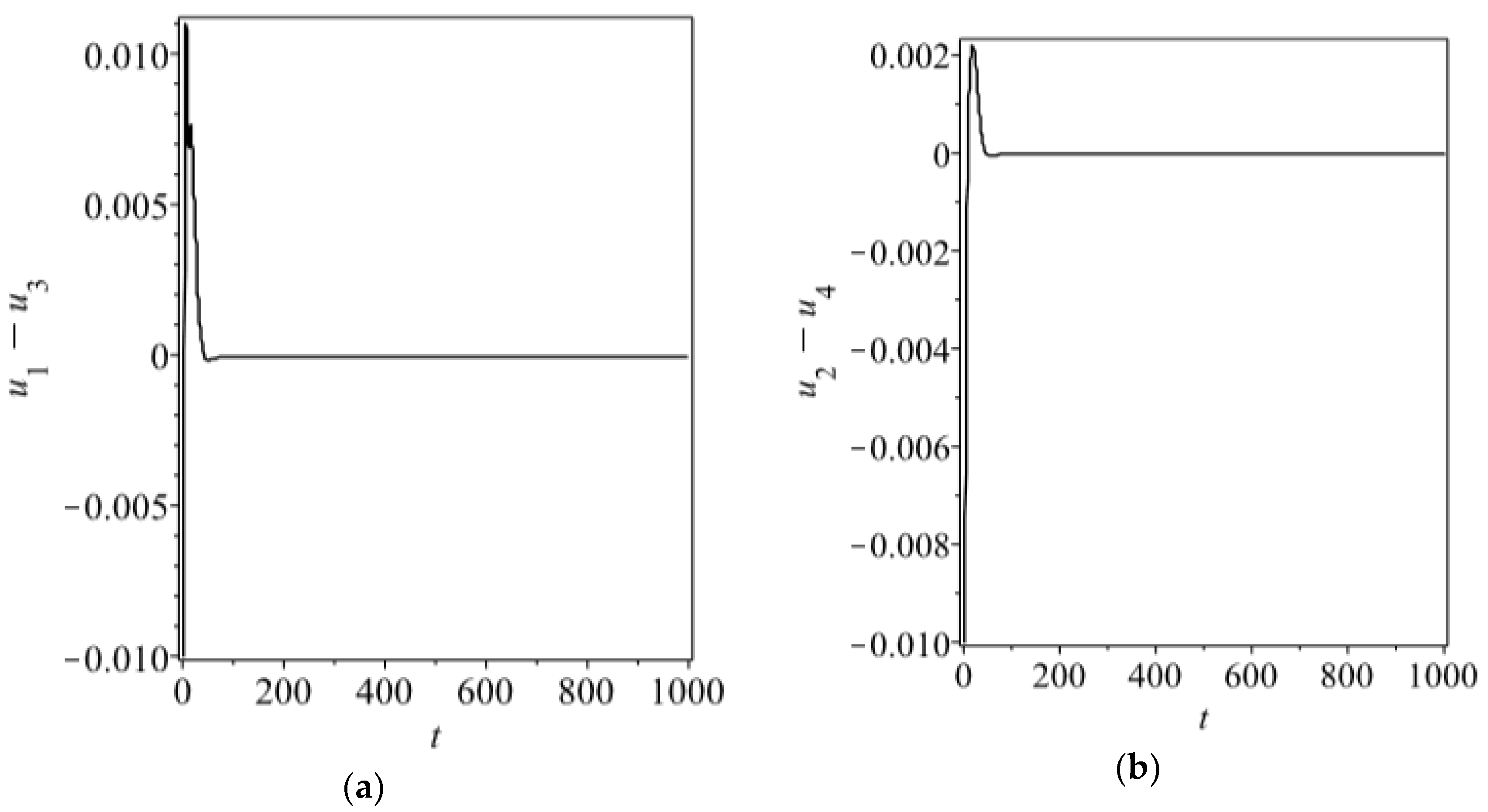
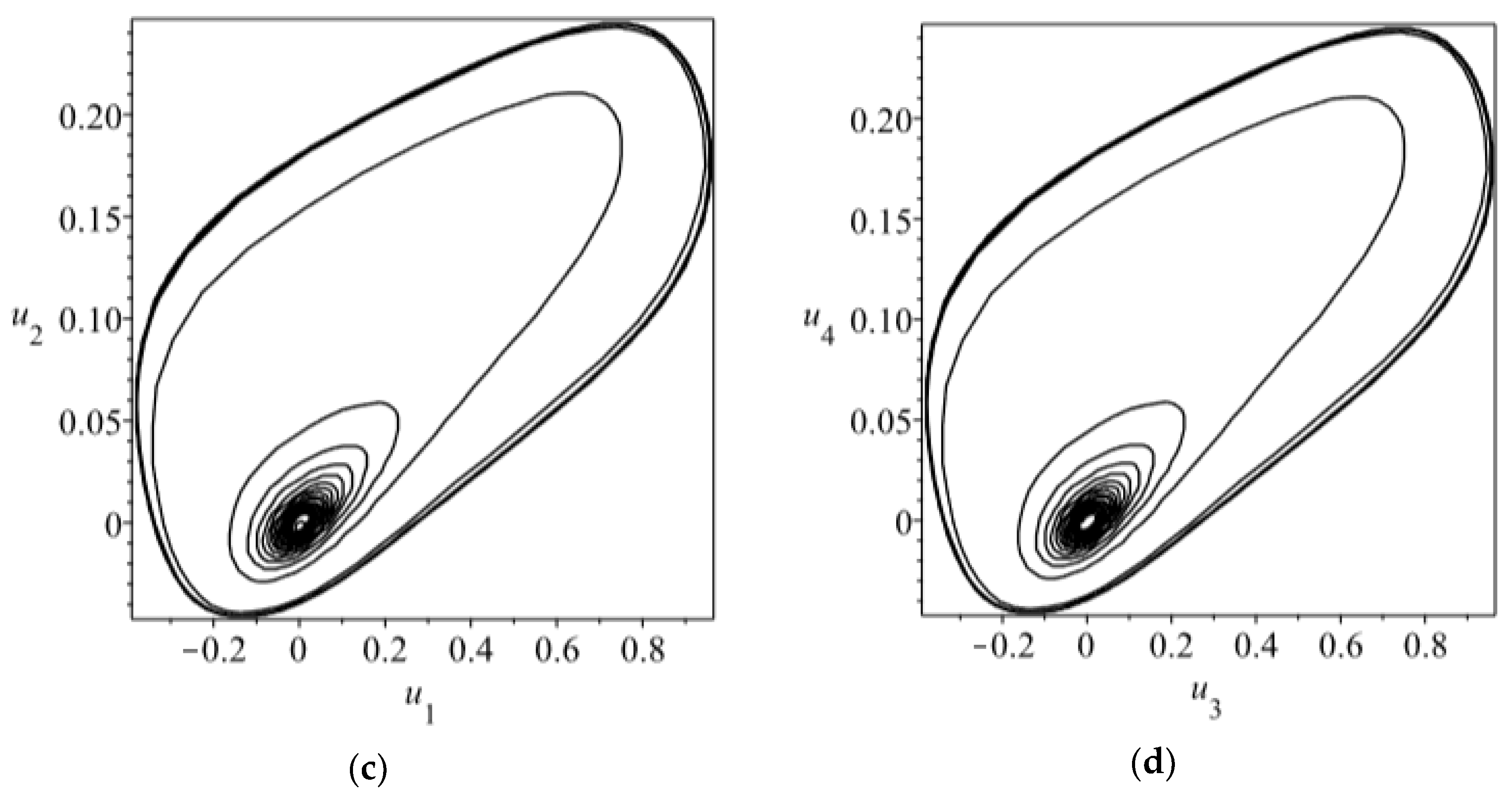
The transversality condition (Equation (26)) holds only when ${\omega }_2=0.335$ and ${\tau }_2=4.149$. Then we can choose an appropriate value of time delay to satisfy the synchronization condition (20), for instance, $\tau =7$. In addition, the initial conditions are taken by $u_1(t-\tau )=0.01$, $u_2(t-\tau )=0$, $u_3(t-\tau )=0.02$, $u_4(t-\tau )=0.01$ for $t\in (-\tau$,$0]$ in the numerical simulations. We present the synchronization errors and phase diagrams of Equation (12) for $c=0.16$ and $c=0.18$ in Figure 3 and Figure 4, respectively, which demonstrate the validity of the synchronization condition (Equation (20)) for Equation (12).

Remark 2.

In this section, we apply the energy method to obtain the synchronization condition for Equation (12), in which the time delay of signal transmission between two neurons is taken into account. The time delay in the signal transmission is involved in the synchronization conditions, the change of which can dramatically affect the synchronous dynamics of two coupled FHN neurons. Comparing the analysis results in this section with the results from Section 2 (see Figure 1, Figure 2, Figure 3 and Figure 4), it is clear that time delay in signal transmission can be used to control the appearance of synchronous spikes in Equation (12).

4. Conclusions

In this paper, we investigate synchronization between two FHN neurons by using the energy method to estimate the influence of time delay in signal transmission on synchronization conditions and synchronous dynamics. According to the concept of the energy method, we can calculate the change rate of energy of the synchronization error system from the original system. If the rate of change of the energy varies periodically, the energy will remain unchanged in one period. Since the energy change rate of the error system can be divided into two parts (periodic and non-periodic), we only need to consider the non-periodic part to determine the evolution tendency of the error system’s energy. The error system’s energy will eventually disappear if the non-periodic part is less than zero. According to this line of thinking, we first derive the synchronization criterion for two coupled FHN neurons without time delay in signal transmission. Analytical and numerical results indicate that it is a feasible approach, to derive synchronization conditions by calculating the rate of change of energy of synchronization error system. Our analysis shows that if time delay in signal transmission is ignored in two coupled FHN neurons, synchronous spikes do not occur for any given coupling strength.

Further investigation shows that the energy method is also valid for the delay differential system. A synchronization condition depending on time delay can be derived if the neural system has an unstable trivial equilibrium. Our research suggests that the existence of the time delay in signal transmission can not only slightly change the synchronization range of coupling strength, but also affect the synchronous dynamics. The two FHN neurons can easily control the occurrence of synchronous spikes or neural rest by only adjusting the time delay in signal transmission. The research result helps us to understand the regulatory mechanisms of synchronization and the synchronous dynamics of neural networks.

In addition, it is worth pointing out that the method of analysis used in this paper can be easily developed to judge synchronization of N coupled FHN neurons. For N coupled FHN neurons, we need to calculate the rate of change of the energy of the error system, consisting of N–1 second-order differential equations with or without time delay. This is feasible for small calculation quantities.

References

1. Hodgkin, A.L.; Huxley, A.F. A quantitative description of membrane current and its application to conduction and excitation in nerve. J. Physiol. 1952, 117, 500–544. [Google Scholar] [CrossRef] [PubMed]
2. Izhikevich, E.M. Which model to use for cortical spiking neurons? IEEE Trans. Neural Netw. 2004, 15, 1063–1070. [Google Scholar] [CrossRef]
3. Fitzhugh, R. Mathematical models of threshold phenomena in the nerve membrane. Bull. Math. Biophys. 1955, 17, 257–278. [Google Scholar] [CrossRef]
4. Bautin, A.N. Qualitative investigation of a particular nonlinear system. J. Appl. Math. Mech. 1975, 39, 606–615. [Google Scholar] [CrossRef]
5. Bin, Z.; Jian, X. Simple zero singularity analysis in a coupled FitzHugh-Nagumo neural system with delay. Neurocomputing 2010, 73, 874–882. [Google Scholar] [CrossRef]
6. Bin, Z.; Jian, X. Fold-Hopf bifurcation analysis for a coupled FitzHuang-Nagumo neural system with time delay. Int. J. Bifurc. Chaos 2010, 20, 3919–3934. [Google Scholar] [CrossRef]
7. Zhen, B.; Xu, J. Bautin bifurcation analysis for synchronous solution of a coupled FHN neural system with delay. Commun. Nonlinear Sci. Numer. Simulat. 2010, 15, 442–458. [Google Scholar] [CrossRef]
8. Swadlow, H.A.; Waxman, S.G. Axonal conduction delays. Scholarpedia 2012, 7. [Google Scholar] [CrossRef]
9. Dhamala, M.; Jirsa, V.K.; Ding, M. Enhancement of neuralsynchrony by time delay. Phys. Rev. Lett. 2004, 92, 074104.1–074104.4. [Google Scholar] [CrossRef]
10. Izhikevich, E.M. Phase models with explicit time delays. Phys. Rev. E 1998, 58, 905–908. [Google Scholar] [CrossRef] [Green Version]
11. Han, Q.; Yang, T.; Zeng, C.; Wang, H.; Liu, Z.; Fu, Y.; Zhang, C.; Tian, D. Impact of time delays on stochastic resonance in an ecological system describing vegetation. Phys. A 2014, 408, 95–105. [Google Scholar] [CrossRef]
12. Song, Z.; Wang, C.; Zhen, B. Codimension-two bifurcation and multistability coexistence in an inertial two-neuron system with multiple delays. Nonlinear Dyn. 2016, 85, 2099–2113. [Google Scholar] [CrossRef]
13. Song, Z.; Xu, J. Codimension-two bursting analysis in the delayed neural system with external stimulations. Nonlinear Dyn. 2012, 67, 309–328. [Google Scholar] [CrossRef]
14. Zhang, X.; Han, Q.; Seuret, A.; Gouaisbaut, F.; He, Y. Overview of recent advances in stability of linear systems with time-varying delays. IET Control Theory Appl. 2019, 13, 1–16. [Google Scholar] [CrossRef]
15. Zhang, X.; Han, Q.; Ge, X.; Ding, D. An overview of recent developments in Lyapunov-Krasovskii functionals and stability criteria for recurrent neural networks with time- varying delays. Neurocomputing 2018, 313, 392–401. [Google Scholar] [CrossRef]
16. Zigen, S.; Jian, X.; Bin, Z. Multitype activity coexistence in an inertial two-neuron system with multiple delays. Int. J. Bifurc. Chaos 2015, 25. [Google Scholar] [CrossRef]
17. Song, Z.; Xu, J. Stability switches and Bogdanov-Takens bifurcation in an inertial two-neurons coupling system with multiple delays. Sci. China Technol. 2014, 57, 893–904. [Google Scholar] [CrossRef]
18. Anderson, H.; Juliana, V.S.; Cesar, M.; Holokx, A.A. Numerical bifurcation analysis of two coupled FitzHugh-Nagumo oscillator. Eur. Phys. J. B 2014, 87. [Google Scholar] [CrossRef]
19. Jia, J.; Liu, H.; Xu, C.; Yan, F. Dynamic effects of time delay on a coupled FitzHugh-Nagumo neural system. Alex. Eng. J. 2015, 54, 241–250. [Google Scholar] [CrossRef]
20. Gan, C.B.; Matjaz, P.; Wang, Q. Delay-aided stochastic multiresonances on scale-free FitzHugh Nagumo neural networks. Chin. Phys. B 2010, 19, 040508.1–040508.6. [Google Scholar] [CrossRef]
21. Jun, M.; Jun, T. A review for dynamics in neuron and neural network. Nonlinear Dyn. 2017, 89, 1569–1578. [Google Scholar] [CrossRef]
22. Ma, J.; Tang, J. A review for dynamics of collective behaviors of network of neurons. Sci. China Technol. Sci. 2015, 58, 2038–2045. [Google Scholar] [CrossRef]
23. Ma, J.; Mi, L.; Zhou, P.; Xu, Y.; Hayat, T. Phase synchronization between two neurons induced by coupling of electromagnetic field. Appl. Math. Comput. 2017, 307, 321–328. [Google Scholar] [CrossRef]
24. Ma, J.; Wu, F.; Wang, C. Synchronization behaviors of coupled neurons under electromagnetic radiation. Int. J. Mod. Phys. B 2017, 31. [Google Scholar] [CrossRef]
25. Lian, H.; Xiao, S.; Wang, Z.; Zhang, X.; Xiao, H. Further results on sampled-date synchronization control for chaotic neural networks with actuator saturation. Neurocomputing 2019, in press. [Google Scholar] [CrossRef]
26. White, J.A.; Chow, C.C.; Rit, J.; Soto-Trevino, C.; Kopell, N. Synchronization and oscillatory dynamics in heterogeneous, mutually inhibited neurons. J. Comput. Neuronsci. 1998, 5, 5–16. [Google Scholar] [CrossRef]
27. Shyam, K.J.; Shaunak, S.; Indra, N.K. Synchronization of coupled oscillator dynamics. IFAC-PapersOnLine 2016, 49, 320–325. [Google Scholar] [CrossRef]
28. Wang, Q.; Lu, Q.; Chen, G.; Feng, Z.; Duan, L. Bifurcation and synchronization of synaptically coupled FHN models with time delay. Chaos Soliton Fract. 2019, 39, 918–925. [Google Scholar] [CrossRef]
29. Rosenblum, M.G.; Pikovsky, A.S.; Kurths, J. Phase synchronization of chaotic oscillators. Phys. Rev. Lett. 1996, 76, 1804–1807. [Google Scholar] [CrossRef] [PubMed]
30. Yanchuk, S.; Maistrenko, Y.; Lading, B.; Mosekilde, E. Effects of a parameter mismatch on the synchronization of two coupled chaotic oscillators. Int. J. Bifurcat. Chaos 2000, 10, 2629–2648. [Google Scholar] [CrossRef]
31. Wang, Y.; Ma, J.; Xu, Y.; Wu, F.; Zhou, P. The Electrical Activity of Neurons Subject to Electromagnetic Induction and Gaussian White Noise. Int. J. Bifurcat. Chaos 2017, 27, 1750030.1–1750030.12. [Google Scholar] [CrossRef]
32. Shih, C.W.; Tseng, J.P. A general approach to synchronization of coupled cells. SIAM J. Appl. Dyn. Syst. 2013, 12, 1354–1393. [Google Scholar] [CrossRef]
33. Campbell, S.A.; Ncube, I.; Wu, J. Multistability and stable asynchronous periodic oscillations in a multiple-delayed neural system. Phys. D 2006, 214, 101–119. [Google Scholar] [CrossRef]
34. Pecora, M.L.; Carroll, T.L. Master stability functions for synchronization coupled systems. Phys. Rev. Lett. 1998, 80, 2109–2112. [Google Scholar] [CrossRef]
35. Chen, M. Synchronization in time-varying networks: A matrix measure approach. Phys. Rev. E 2007, 76, 016104.1–016104.10. [Google Scholar] [CrossRef]
36. Lu, W.L.; Chen, T.P. New approach to synchronization analysis of linearly coupled ordinary differential systems. Phys. D 2006, 213, 214–230. [Google Scholar] [CrossRef]
37. Li, L.; Ye, H. Energy method for computing periodic solutions of strongly nonlinear autonomous systems with multi-degree-of-freedom. Nonlinear Dyn. 2003, 31, 23–47. [Google Scholar] [CrossRef]
38. Kakiuchi, N.; Tchizawa, K. On an explicit duck solution and delay in the FitzHugh-Nagumo equation. J. Diff. Eq. 1997, 114, 327–339. [Google Scholar] [CrossRef]
39. Zhen, B.; Xu, J.; Song, Z. Lateral periodic vibrations of footbridges under crowd excitation. Nonlinear Dyn. 2016, 86, 1701–1710. [Google Scholar] [CrossRef]
40. Karaoglu, E.; Yilmaz, E.; Merdan, H. Hopf bifurcation analysis of coupled two-neuron system with discrete and distributed delays. Nonlinear Dyn. 2016, 85, 1039–1051. [Google Scholar] [CrossRef]
41. Li, X.; Hu, G. Stability and Hopf bifurcation on a neuron network with discrete and distributed delays. Appl. Math. Sci. 2011, 5, 2077–2084. [Google Scholar] [CrossRef]
42. Yang, L.; Hou, X.R.; Zeng, Z.B. A complete discrimination system for polynomials. Sci. China E 1996, 39, 628–646. [Google Scholar] [CrossRef]
43. Yang, L.; Hou, X.R.; Zeng, Z.B. An alternative algorithm for determining the number of real roots of a polynomial. In Proceedings of the International Workshop on Logic and Software Engineering; World Scientific: Singapore, 1996. [Google Scholar]
Figure 1. Dynamics of Equation (2) with a = 0.1 , b = 0.08 , γ = 3 , c = 0.16 . The initial conditions are taken as u 1 ( 0 ) = 0.01 , u 2 ( 0 ) = 0 , u 3 ( 0 ) = 0.02 , u 4 ( 0 ) = 0.01 ; (a) u 1 ( t ) vs. t ; (b) u 2 ( t ) vs. t ; (c) u 3 ( t ) vs. t ; (d) u 4 ( t ) vs. t .
Applsci 09 02159 g001aApplsci 09 02159 g001b
Figure 2. Dynamics of Equation (2) with a = 0.1 , b = 0.08 , γ = 3 , c = 0.18 . The initial conditions are taken as u 1 ( 0 ) = 0.01 , u 2 ( 0 ) = 0 , u 3 ( 0 ) = 0.02 , u 4 ( 0 ) = 0.01 . (a) u 1 ( t ) vs. t ; (b) u 2 ( t ) vs. t ; (c) u 3 ( t ) vs. t ; (d) u 4 ( t ) vs. t .
Applsci 09 02159 g002aApplsci 09 02159 g002b
Figure 3. Synchronization errors (a,b) and phase diagrams (c,d) for Equation (12) with a = 0.1 , b = 0.08 , γ = 3 , c = 0.16 and τ = 7 . The initial conditions are chosen as u 1 ( t τ ) = 0.01 , u 2 ( t τ ) = 0 , u 3 ( t τ ) = 0.02 , u 4 ( t τ ) = 0.01 for t ( τ , 0 ] .
Applsci 09 02159 g003aApplsci 09 02159 g003b
Figure 4. Synchronization errors (a,b) and phase diagrams (c,d) for Equation (12) with a = 0.1 , b = 0.08 , γ = 3 , c = 0.18 and τ = 7 . The initial conditions are chosen as u 1 ( t τ ) = 0.01 , u 2 ( t τ ) = 0 , u 4 ( t τ ) = 0.01 , u 4 ( t τ ) = 0.01 for t ( τ , 0 ] .
Applsci 09 02159 g004