1. Introduction
The increasing use of distributed renewable energy sources (RES) is one of the primary steps towards the global transition to the smart grid paradigm [
1,
2]. On the other hand, uncertainties and intermittency of RES result in unpredictable electricity generation profiles having an impact on power system balance and stability [
3]. There are many technological and economic issues associated with high rates of renewables penetration in the electrical grid; in particular, daily and seasonal fluctuations in energy production and load demand profiles, high cost of energy storage, and the delicate balance between grid reliability and flexibility are among the most troubling aspects [
4,
5].
To deal with such issues, suitable Energy Management Systems (EMSs) have been discussed in the technical literature [
6,
7,
8]. The key functions of EMSs are monitoring and optimization of power flows. These systems, at the end-user level, allow customers to play an active role in the energy market. On the other hand, they provide support to the grid operator in terms of optimized decisions, for example implementing Demand Side Management schemes [
9,
10].
Along with the industrial and commercial sectors, EMSs are also advantageous in the context of smart homes, where different kinds of system components (i.e., hardware elements, software algorithms, network connections, and sensors) cooperate with each other to provide various services supporting human lifestyle [
11]. An EMS should exhibit distinct features to be engaging for end users. Besides providing a commodity and an advantage, it should seamlessly integrate with the ecosystem of home devices and appliances, it should require an effortless setup and a small amount of wiring, and it should not be bulky. Therefore, besides the research on the functional aspects of EMSs (e.g., how they are defined, what they optimize, and which strategy they use), for their real-world adoption, it is important to investigate how to perform their embedded implementation and to integrate them into a smart home more easily. To this aim, the Internet of Things (IoT) paradigm is currently the favored solution.
However, most works on EMSs disregard these aspects and focus solely on the implementation of support technologies (e.g., networking, smart metering, controllable devices and appliances), or architectural aspects. In fact, networking technologies such as Home Area Networks (HAN) or Personal Area Networks (PAN) are extensively studied to enable the implementation of EMSs [
12,
13]. Furthermore, some authors focus on the implementation of smart devices that support the interaction with an EMS. For example, the embedded implementation of network-enabled Battery Management System (BMS) is presented in [
14]. Instead, Ozadowicz and Grela [
15] proposed a smart meter that uses the IoT paradigm to provide a universal device interface. Other examples of IoT system prototypes have been proposed in the technical literature for home automation and energy monitoring inside the smart home/building [
16,
17,
18].
Several works propose architectural approaches for the smart integration of appliances, devices, and energy management facilities. For example, Khamphanchai et al. [
19] proposed a platform for energy management of buildings that is based on distributed agents. Furthermore, architectures based on the IoT paradigm are presented in [
20,
21]. A cloud-based architecture that permits data collection, control of appliances, and the definition of EMSs as cloud-based services is presented in [
22]. Following a similar approach, Al Faruque and Vatanparvar [
23] and Yaghmaee Moghaddam and Leon-Garcia [
24] proposed architectures based on fog computing [
25]. In particular, Al Faruque and Vatanparvar [
23] proposed the concept of energy management as a service.
Few works have proposed embedded implementations of EMSs. The authors of [
26] implemented an optimization algorithm on embedded devices but did not describe the details of the algorithm. Other works implemented just rule-based EMSs or short-term controllers. For example, some works implemented very simple on/off appliance switching functionalities based either on the hour of the day and the presence of users [
27] or on a user-selected power consumption limit [
28]. In other works, more complex EMSs are proposed. However, only the rule-based short-term layer of the EMS are implemented on microcontrollers, whereas the medium- and long-term layers run on a centralized outside-of-the-house controller [
29] or a dedicated PC [
30]. A more sophisticated approach is presented in [
31,
32], which implement EMSs on microcontrollers to perform load-shifting. These EMSs, however, do not use optimization techniques but a set of preprogrammed rules (fuzzy or deterministic). Although this choice simplifies the implementation, the obtained results are suboptimal in the medium/long term. To the authors’ knowledge, the literature misses a detailed description of an embedded EMS implementation that optimizes power flows among renewable generators, loads, and storage systems.
To provide a further step towards the real-world deployment of EMSs, this paper presents an embedded implementation and an extended validation of the EMS proposed in [
33]. This EMS is very promising because it provides advantages for both the end user and the utility. In fact, it applies optimization algorithms: (1) to obtain a reduction of the end user’s electricity bill; and (2) to reduce the uncertainty, due to forecasting errors, on the daily profile of the power exchanged between the user and the public utility. The EMS is designed to preserve user habits and to require little communication with the grid manager. These are some of the key requirements for the domestic adoption of an EMS. However, another important requirement is the easy connection to home appliances and to the grid manager. To this aim, it is advantageous to implement the EMS as an IoT device (rather than as a software module of the smart meter) that connects wirelessly to the appliances’ sensors and actuators and exposes its services to the grid manager and the user [
34].
For the above reasons, the EMS proposed in [
33] is particularly suitable for the smart home context. Therefore, the main aim of the present paper is the embedded implementation of such an EMS in order to make it compatible with the IoT paradigm. To this aim, the EMS must be redesigned guaranteeing a feasible implementation and the optimality of the results. Specifically, Di Piazza et al. [
33] used Mixed Integer Linear Programming (MILP) and exhibited software dependencies from third-party solvers, which are currently unavailable for embedded platforms; thus, MILP should be replaced with other techniques that do not impose such dependencies.
In general, other authors use heuristic algorithms such as Particle Swarm Optimization to implement EMSs [
35,
36]. These algorithms are quite simple and do not depend on third-party solvers, thus they satisfy the feasibility requirement. However, these authors only perform simulations and do not make an embedded implementation. In any case, heuristics-based algorithms can get stuck in local optima and do not always return the global optimum; therefore, they do not ensure the optimality of the results.
Based on such considerations, in this paper, the algorithm of Di Piazza et al. [
33] is completely re-implemented using Dynamic Programming (DP) instead of MILP. The EMS is implemented and tested on a Raspberry Pi board [
37], but can also run on any other Linux-based embedded platform. Its experimental validation was performed connecting it to a network of wireless sensors and actuators based on Wemos boards [
38]. The differences between this paper and the work in [
33] can be summarized as follows:
DP is used instead of MILP for the previously explained reasons.
Instead of considering only one dwelling, the EMS performance was evaluated considering a small grid of four smart homes; this aimed at measuring the increased advantage from the point of view of the utility when several users adopt the EMS.
The EMS performance was also assessed experimentally by connecting it to a network of wireless sensors according to the IoT paradigm.
The goal of the investigation was twofold: (1) evaluating the theoretical and measured computational efficiency, showing the real-world feasibility of the implemented EMS; and (2) measuring the effectiveness of the EMS for both the utility and the users during a 30-day period.
The paper is organized as follows. The fundamentals of the chosen EMS are highlighted in
Section 2, and the case study is described in
Section 3.
Section 4 is focused on the embedded implementation of the EMS. After describing the chosen embedded platform and the test bench,
Section 5 presents and discusses the experimental results. Finally, some conclusions are drawn.
2. Fundamentals of the Chosen EMS
The chosen EMS has been presented in [
33]; for the sake of brevity, only the main features and the optimization problems are recalled in the following.
2.1. Main Features
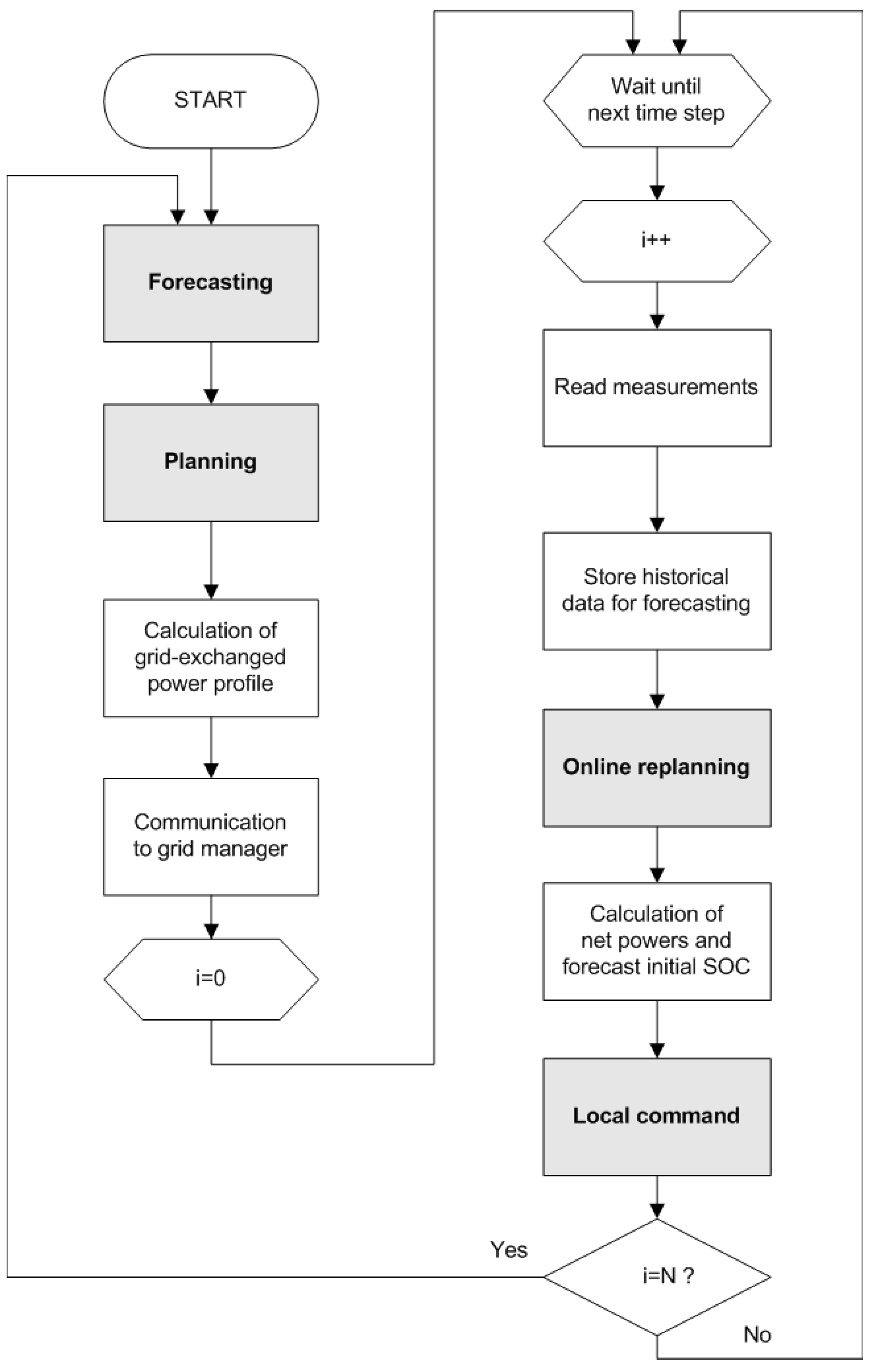
The flowchart of the chosen EMS is shown in
Figure 1. As for many EMSs, the processing starts with the
Forecasting stage, in which the 24-h ahead profiles of load demand and environmental variables tied to renewable generation are forecast on the basis of past data. To achieve good results, the
Forecasting stage of the chosen EMS is based on the Nonlinear AutoRegressive network with eXogenous inputs (NARX). This Artificial Neural Network (ANN) has been successfully used in time-series modeling thanks to its simple implementation and its adaptive learning process, even with small-scale data [
39,
40,
41]. In the considered case, the exogenous input is the environmental temperature.
The subsequent optimization stage considers forecast load demand and plans to satisfy it while pursuing the chosen goals. This stage is split into two tasks, i.e., Planning and Online Replanning, aiming to provide advantages both to the end user and to the grid manager at the same time.
The Planning task optimizes the user’s cash flow (CF) over the planned period (24 h) and produces a set of power reference values, one for each system component (i.e., electrical loads, storage systems, and renewable generators). In other EMSs, this set is directly sent to lower level devices that perform the instantaneous control of the hardware. This approach, therefore, neglects forecasting errors. Instead, in the chosen EMS, the output of the Planning task is only used to compute the optimal Grid-Exchanged Power Profile (GEPP) for the whole next day. The GEPP is a vector of power values across the time steps of a day. In particular, these values are positive when the grid supplies the smart house, or negative when the power from renewable generators is injected into the grid. The planned GEPP is transmitted over the Internet to the grid manager as an obligation, to which the user commits himself.
Then, the Online Replanning task is repeated during each 24 h cycle. It aims at minimizing the deviation between the actual and the transmitted GEPPs and computes the actual set of power references to obtain this goal. These values are delivered to the different system components by the Local Command stage via an internal HAN. Besides minimizing the user’s cash flow, the proposed EMS reduces the uncertainty on the GEPP thanks to its Online Replanning stage. The public utility can exploit this last feature to optimize power generation/distribution and to improve its economic policy planning.
2.2. Optimization Problems
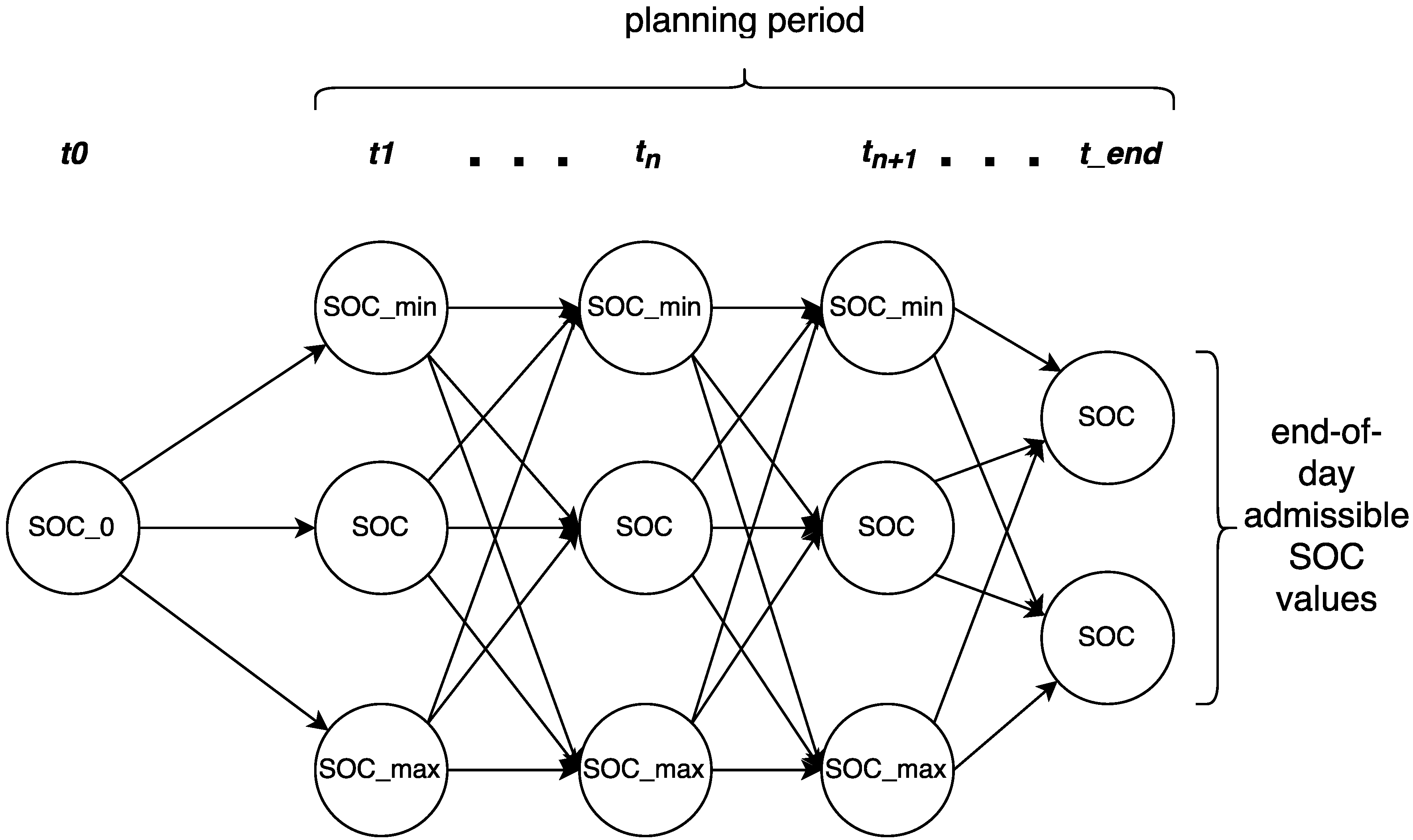
Both Planning and Online Replanning tasks are executed solving optimization problems. The considered variables are the battery state of charge (SOC) and the power flows between couples of system devices: loads, renewable generators, battery storage systems, and connection to the public grid.
In the optimization problem of the
Planning stage, the objective function is the end user’s cash flow (
), which is expressed as:
where
and
are the prices of sold/purchased energy, respectively;
is the duration of each time step;
t is a discrete variable representing the time step index; and
N is the number of time steps in a day.
The objective function in Equation (
1) must be minimized satisfying a set of physical and design constraints at each time step, namely:
non-negative value for each variable;
power balance at generation node;
power balance at load node;
maximum contractual grid-exchanged power;
maximum battery charging/discharging power;
minimum and maximum SOC values;
continuity of SOC between consecutive days;
evolution of SOC between time steps; and
cyclicity of SOC profile between consecutive days.
The optimization problem of the
Online Replanning stage aims at finding the solution that minimizes the maximum deviation between the actual GEPP and the self-committed GEPP (
). Such a deviation is due to forecasting errors. Hence, the objective function to minimize is:
To avoid greedy minimization of instantaneous differences, at each execution, the algorithm decides the variable values for the current time step (using measurements) and also for the following steps (using forecast values). However, only the reference power values for the current time step () are sent to the hardware, whereas the other values (for ) are discarded.
The constraints for Equation (
3) are readily adapted from those of the
Planning stage by:
3. The Case Study
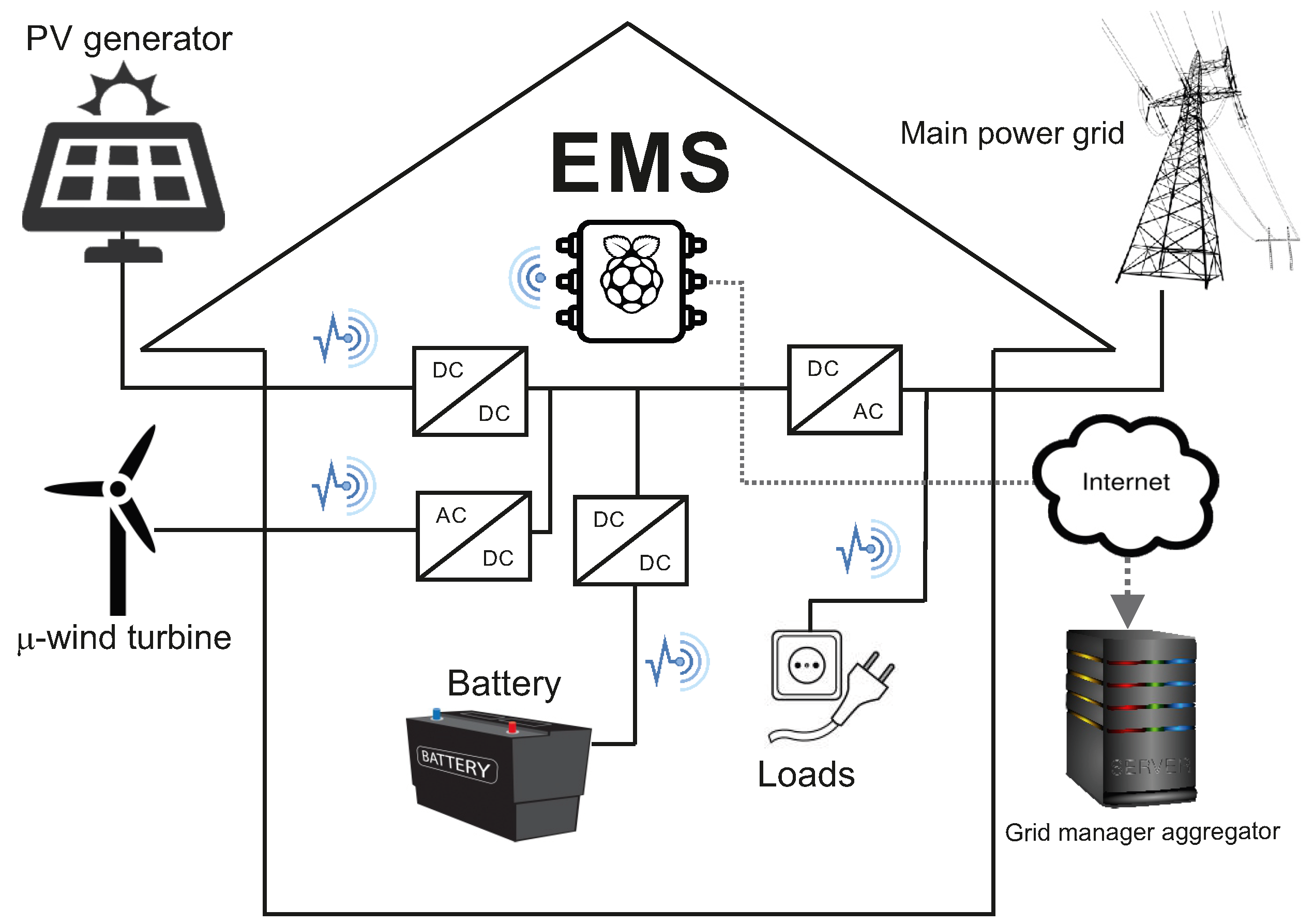
The proposed technique was illustrated and validated referring to a small electrical grid that encompasses four networked dwellings. Each smart home was equipped with an EMS of the proposed type, which generated in real time the references for the power flows among the system components: loads, renewable generators, and battery storage systems. Furthermore, a series of previously devised wireless sensors [
38] was connected to the electric appliances to send measured data to the EMS and to forward the power references set by the EMS to the power electronic converters that interface system components. The wireless sensors communicated using Message Queue Telemetry Transport (MQTT), a lightweight messaging protocol for the IoT based on the publish-subscribe paradigm. A pictorial view of each smart home is shown in
Figure 2.
The four users (A÷D) had different habits, hence different load profiles. The main parameters of the system under study are shown in
Table 1, and the following working assumptions were made:
The aggregated load profile is considered as an input; if needed, a lower-level control system can shift or schedule each load, while respecting the aggregated load profile.
The maximum contractual power for Users A and C is 3 kW, whereas for Users B and D it is 4 kW.
Each user has only one renewable generator; in particular, Users A and B have PV generators, whereas Users C and D have micro Wind Energy Conversion Systems (WECSs).
The renewable generators are always operated in the maximum power point for each environmental condition (wind speed, solar irradiance, and temperature) since they are usually equipped with maximum power point trackers (MPPT).
Transferring power from the battery to the grid is not allowed by the utility, according to the technical rule for grid-connection in force in some European countries at the time of writing.
The battery must be small and affordable for the end user, thus it is not suitable to sustain hours-long islanding; the considered capacity values for each user are given in
Table 1.
Such working assumptions did not affect the general validity of the proposed EMS. With regard to Points 1 and 4, even if slight deviations occurred (e.g., the lower-level control system does not precisely respect the aggregated load profile or the renewable generator does not work exactly in its maximum power point), they were seen as forecasting errors. Hence, using the battery as an energy buffer, they were effectively corrected by the
Online Replanning stage of the EMS, as happens for errors due to unexpected weather fluctuations [
42]. As for Point 3, in the presence of more than one renewable generator, their power profiles could be aggregated following the same approach used for loads. However, this scenario is highly unusual in the smart home context because it would be very expensive. Finally, with regard to Point 6, the influence of battery size on the EMS performance has been already studied in [
42], where a sensitivity analysis has been performed.
To send the self-committed GEPP once a day, each of the four smart homes was connected to the data aggregator of the grid manager through a secure Internet connection [
13]. The data aggregator received and aggregated the user-committed GEPPs; the resulting profile could be exploited by the utility to improve its policy planning.
5. Experimental Verification and Results
A dedicated test bench was set up to validate the embedded implementation of the chosen EMS under the hypothesis of controlling four smart homes of the type described in
Section 3. Such a test bench is described in detail in the following subsection.
The input data came from publicly available datasets. Outdoor temperature, solar irradiance, and wind speed data came from the U.S. National Solar Radiation Database [
47], whereas load demand data came from [
48]. Prices for sold and purchased energy were retrieved from [
49]. The data considered for the study referred to the city of Amarillo TX, USA. Given each dataset, a first part of the data was used to train and validate the related ANN. The remaining part was considered as the set of instantaneous measurements to be compared with the forecast profile.
The electrical behavior of the appliances of each smart home was emulated by the related wireless sensors, as explained in the following subsection. This approach was followed because the main aim of the work was to assess whether the EMS can run on the embedded platform, perform its computation within the required time frame, and exchange data with the wireless sensors.
5.1. Test Bench Description
Four EMSs of the proposed type were implemented on four Raspberry Pi 3 model B boards running the Linux operating system. This embedded platform was based on a quad-core Broadcom BCM2837 64-bit CPU clocked at 1.2 GHz and has 1 GB of RAM. Furthermore, it provides an onboard WiFi connection, a gigabit Ethernet port, and a Micro SD port to boot the Linux operating system [
37]. As an alternative, the proposed EMS could be easily executed on other Linux-based embedded platforms such as the Zedboard [
50] by just recompiling the same source code.
The wireless sensors used in the test bench have been previously devised in [
38] and are based on Wemos D1 mini pro boards. These boards encompass an ESP8266 system-on-chip by Espressif Systems, which includes a low-cost IEEE 802.11b/g/n Wi-Fi chip with full TCP/IP support and a 32-bit RISC L106 microcontroller. For their use in the field, such devices are appropriately interfaced with physical sensors to acquire the variables of interest (e.g., voltage and current of each appliance, solar irradiance, wind speed, and outdoor temperature). At the same time, they send the appropriate power reference to each power electronic converter, and they read the instantaneous battery SOC. For the present work, instead, such wireless sensors were modified to bypass the physical sensors and to emulate the electrical equipment to which they were connected. In particular, the power profiles of renewable generators and electrical loads were computed on the basis of the considered public datasets. As for the storage system, instead, a simple static battery model was implemented; it is expressed by Equation (
4), and it takes into account battery power reference (
) and charge/discharge efficiency (
) to compute SOC variation. On the other hand, the grid manager’s data aggregator was emulated using a desktop PC connected to the Internet and running a small server application written on purpose.
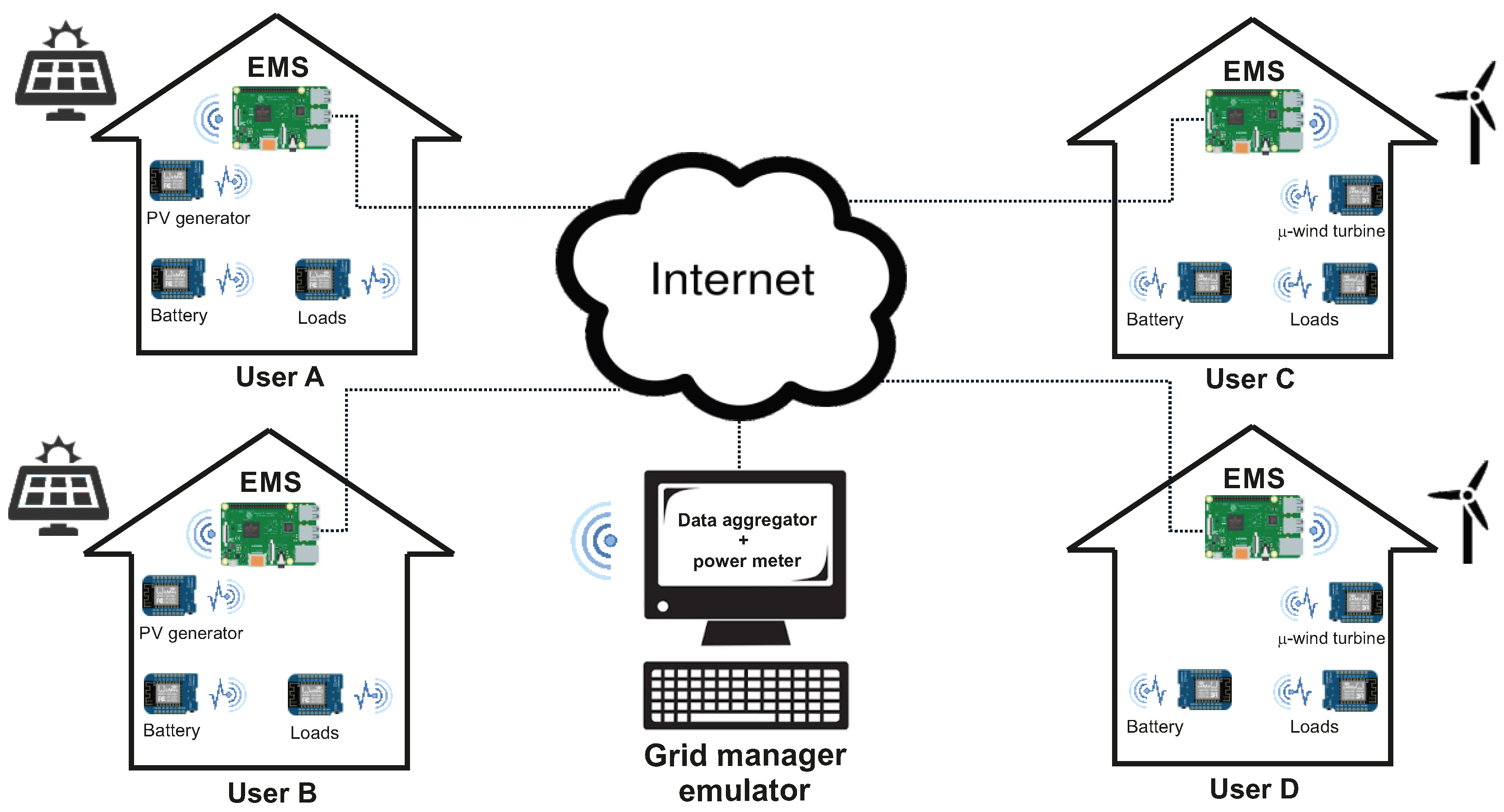
The synopsis of the experimental setup is shown in
Figure 4, and its operation is briefly explained in the following. At the beginning of each considered day, each EMS read the instantaneous measurements of load demand, solar irradiance, and wind speed sent from the wireless sensors. Using these data, it performed the forecasting of renewable generation and load profiles thanks to the NARX ANNs. It executed the
Planning task to compute the self-committed GEPP and sent it to the emulated grid manager’s data aggregator using the Internet connection of the Raspberry Pi. Then, it started performing the
Online Replanning task obtaining power references to control the plant accordingly. In particular, at each time step, it read the current values from the wireless sensors, solved the optimization problem, and sent the power references for the electrical appliances. Given the working assumptions of
Section 3, the battery was the only controllable device in each of the four plants. Hence, each EMS sent the battery power reference to the wireless sensor that emulated the battery power flow and updated the SOC. Then, these two quantities were plotted, as shown in
Section 5.3. Concurrently, the emulated grid manager’s data aggregator performed the following operations:
It listened to the messages with which each EMS sent its self-committed GEPP 24 h ahead via a secure Internet connection.
It retrieved the measured power exchanged by the grid and each user via the network of wireless sensors.
It compared each user-committed GEPP with the corresponding actual GEPP.
It computed the error metrics on each user’s GEPP, which are shown in
Section 5.3.
It computed each user’s cash flow starting from the GEPP.
It compared the aggregated actual GEPP with the aggregated user-committed GEPPs. The two power profiles were then plotted, as shown in
Section 5.3.
5.2. Assessment of EMS Execution Time
The execution time of the Planning and Online Replanning tasks on the chosen embedded platform was measured in four scenarios to consider different sets of EMS parameters. In particular, two values of the SOC discretization step (i.e., 0.2% and 0.5%) and two values of the time step duration (i.e., 15 and 30 min) were considered.
The experimental results of such an analysis are shown in
Table 2 and
Table 3, and they confirm that
Planning is the most computationally intensive operation, as demonstrated in
Section 4.2. The EMS must start and complete the execution of such a task during the last time step of the day. Therefore, its execution time must be smaller than
(i.e., 900 or 1800 s).
Table 2 shows that the execution time of the
Planning task is well below the allowed time frame for the two scenarios with
= 30 min. On the other hand, a SOC discretization step of 0.2% cannot be chosen if the user also wants to set the time step to 15 min.
As for the
Online Replanning task, it has a significantly lower computational complexity. Furthermore, the related execution time decreases during the day. In fact, the number of remaining time steps gets smaller at each execution, and the graph becomes progressively less complex. Therefore, the first time step has the longest execution time of the
Online Replanning task. As
Table 3 shows, the execution of such a task took no more than 2.5 s in all considered scenarios.
On the basis of the results shown in
Table 2 and
Table 3, it is worth estimating whether older Raspberry Pi models are suitable platforms to run the proposed embedded EMS. The constraint to be satisfied is that both
Planning and
Online Replanning tasks should be executed during the last time step of the day. As an example, the scenario with
= 0.2% and
= 30 min was considered. Therefore, the maximum execution time must not exceed 1800 s. The performance degradation index (PDI) due to the use of older Raspberry Pi platforms could be estimated on the basis of benchmark indices such as single-core Million Instructions Per Second (MIPS) and Mega FLoating point Operations Per Second (MFLOPS) values; such indices were retrieved from [
51] and are summarized in
Table 4. The performance of Raspberry Pi 3 model B was compared with that of the other models by computing the MIPS ratio and the MFLOPS ratio. For a more conservative estimation, the PDI was computed as the maximum of such ratios. Then, the execution time of the proposed embedded EMS on each Raspberry Pi platform was estimated by multiplying the PDI by the execution time measured on the Raspberry Pi 3 model B. As
Table 4 shows, the proposed embedded EMS can be executed in all the considered platforms except for the Raspberry Pi 1 model B. Using the same approach, the comparison could be easily extended to the combination of other scenarios and other low-cost embedded platforms for IoT applications [
52].
5.3. Assessment of the EMS Effectiveness
The above described experimental setup was used to assess the effectiveness of the implemented EMS in the scenario with
= 30 min and
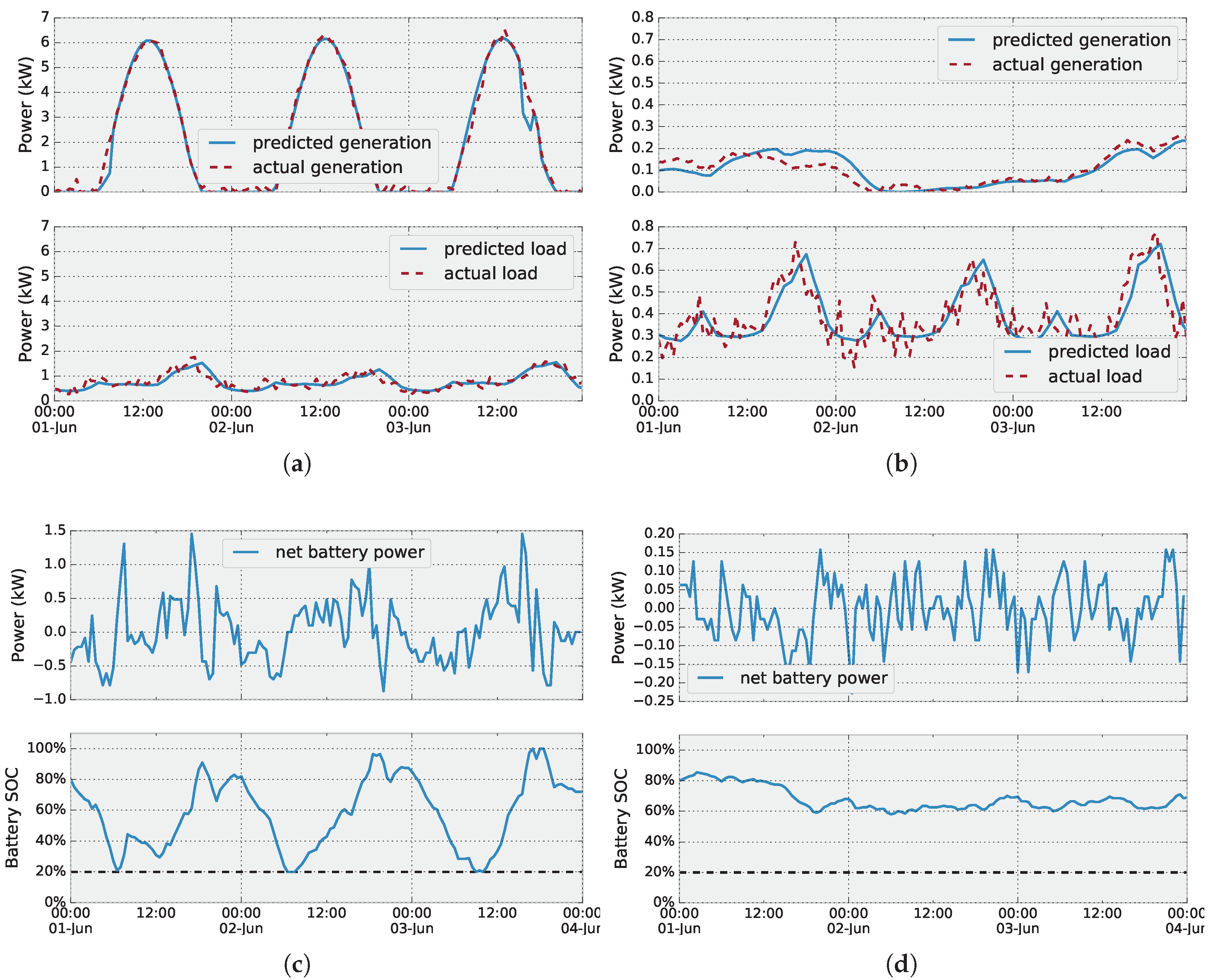
= 0.5%. In fact, slightly better results could be obtained in the other scenarios. At the functional level, the performed tests showed that the EMS correctly interacted with the wireless sensors and the grid manager’s data aggregator. To assess the EMS effectiveness, the uncertainty of the output profile (i.e., the GEPP) must be compared with that of the input profiles (i.e., renewable generation and load demand), and the cash flow variation must be evaluated. The input data for emulating the electric appliances span thirty consecutive days and came from the aforementioned publicly available datasets. As an example,
Figure 5a,b shows the comparison between the forecast profiles and the actual input data for the EMSs of Users B and C for the first three days. These plots are also representative of the other two user profiles.
Two metrics were computed for the forecasting errors, namely the Normalized Root Mean Square Error (NRMSE) and the Normalized Maximum Absolute Error (NMAE). It is worth noting that the error metrics of PV and wind generation were normalized with respect to the nominal power of each renewable generator. On the other hand, error metrics on load demand were normalized with respect to the maximum contractual power. The values of the forecasting error metrics for all users during the 30 days are shown in
Table 5; the maximum NRMSE and NMAE values are about 8% and 50%, respectively. The same table also reports the cumulated errors obtained combining generation and load NRMSE values in quadrature.
As an example of the EMS outputs, the plots of battery power and SOC profiles for Users B and C in the first three days of the considered month are shown in
Figure 5c,d. These plots are also representative of the profiles of the other two users. As expected, the maximum battery charging/discharging powers are not exceeded.
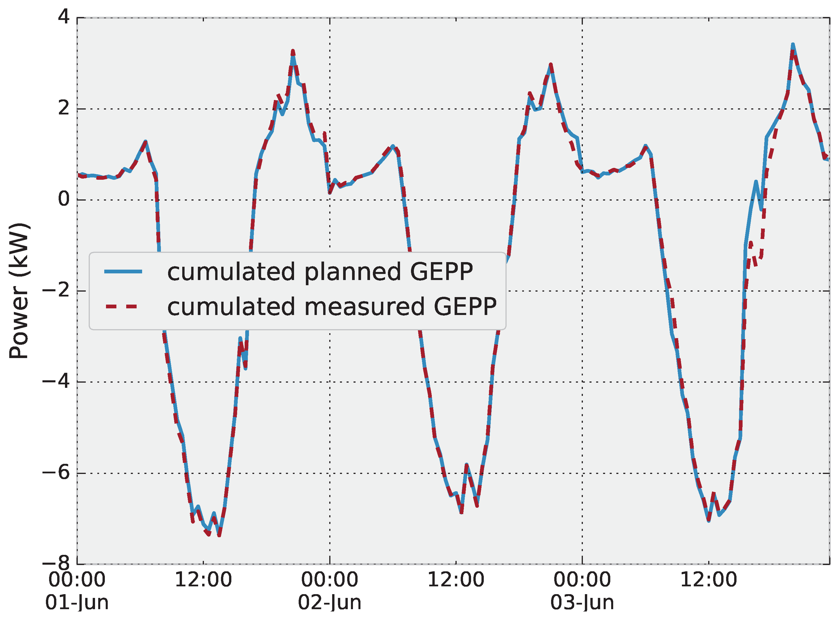
A plot of the aggregated user-committed GEPP versus the actual cumulative grid power in the same three days is shown in
Figure 6. As the figure shows, the two curves overlap each other almost perfectly. Furthermore,
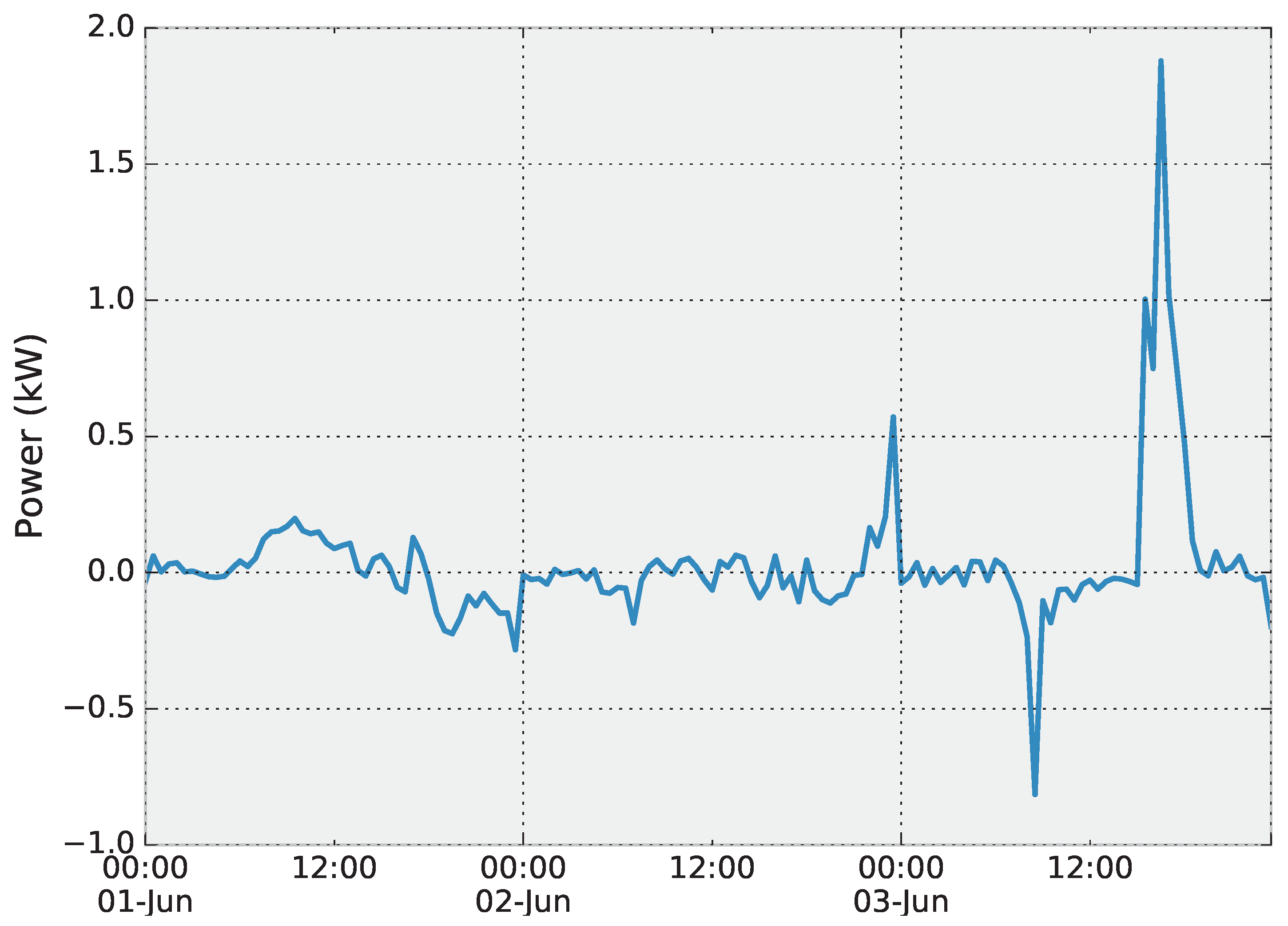
Figure 7 shows the difference between planned and measured aggregated GEPP. In particular, the predictability of the power profile is clearly expressed by the error metrics that were computed on the GEPP, as shown in
Table 6. The normalization factor for the metrics of each user was the maximum contractual power (i.e., 3 kW for Users A and C, and 4 kW for Users B and D). On the other hand, the normalization factor for the cumulative GEPP was the maximum cumulative contractual power, i.e., 14 kW.
It is worth noting that the maximum NRMSE and NMAE values in
Table 6 are about 7% and 55%, respectively. Furthermore, the low NRMSE value on the aggregated profile (2.88%) shows that, from the utility perspective, the uncertainty can be even lower than that of the single households. This result is due to the statistical compensation of users’ deviations, and it also indicates the effectiveness of the EMS for the utility operator.
As an example of the end user’s cash flow, a sample day is discussed, i.e., day 4. Despite the forecasting errors and the effort to adhere to the committed GEPP, User B earns $2.46, i.e., 1.46% more than the income without any EMS; User C, instead, pays $0.70, i.e., 3.23% less than the expense without any EMS. The actual profit of both users could even be higher if economic incentives were proposed by the public utility to reward the uncertainty reduction on the GEPP.
6. Conclusions and Future Perspectives
An embedded and computationally efficient implementation of an EMS for smart homes has been proposed. The chosen EMS algorithm has been redesigned using DP instead of MILP to simplify the implementation process. As demonstrated by a computational complexity analysis, the obtained EMS is suitable for the embedded implementation. Furthermore, the optimality of the solutions has not been compromised in the algorithm redesign.
A suitable test bench was set up to assess the EMS performance in a chosen case study (i.e., four networked dwellings including renewable generators) that was emulated. The experimental results show that the EMS can perform each of its tasks on the embedded platform within the allowed time frames; they also show that the embedded EMS correctly exchanges data with the wireless sensors and the grid manager’s data aggregator. Furthermore, an extended validation of the EMS effectiveness was performed in terms of cash flow increase and uncertainty reduction.
In particular, the experiments showed that the EMS performs its computations in a few minutes for the Planning task and in less than 2.5 s for the Online Replanning task. Furthermore, the EMS performance is very good since the uncertainty on the daily profile of the power exchanged by the users with the utility is significantly mitigated (NMRSE = 2.88% and NMAE = 22%). This result is a first step towards the quick and affordable adoption of EMSs in smart homes.
As for the future development of this work, the short execution times obtained for the proposed embedded EMS suggest that there is sufficient margin to take into account other important aspects such as battery state of health in the EMS formulation. Furthermore, future activities will contemplate testing the embedded EMS on the field, i.e., within real-world smart homes.


