Effects of Varying Noise Levels and Lighting Levels on Multimodal Speech and Visual Gesture Interaction with Aerobots

Featured Application

Patrol, Search, and Rescue Aerial Robots.

Abstract

This paper investigated the effects of varying noise levels and varying lighting levels on speech and gesture control command interfaces for aerobots. The aim was to determine the practical suitability of the multimodal combination of speech and visual gesture in human aerobotic interaction, by investigating the limits and feasibility of use of the individual components. In order to determine this, a custom multimodal speech and visual gesture interface was developed using CMU (Carnegie Mellon University) sphinx and OpenCV (Open source Computer Vision) libraries, respectively. An experiment study was designed to measure the individual effects of each of the two main components of speech and gesture, and 37 participants were recruited to participate in the experiment. The ambient noise level was varied from 55 dB to 85 dB. The ambient lighting level was varied from 10 Lux to 1400 Lux, under different lighting colour temperature mixtures of yellow (3500 K) and white (5500 K), and different background for capturing the finger gestures. The results of the experiment, which consisted of around 3108 speech utterance and 999 gesture quality observations, were presented and discussed. It was observed that speech recognition accuracy/success rate falls as noise levels rise, with 75 dB noise level being the aerobot’s practical application limit, as the speech control interaction becomes very unreliable due to poor recognition beyond this. It was concluded that multi-word speech commands were considered more reliable and effective than single-word speech commands. In addition, some speech command words (e.g., land) were more noise resistant than others (e.g., hover) at higher noise levels, due to their articulation. From the results of the gesture-lighting experiment, the effects of both lighting conditions and the environment background on the quality of gesture recognition, was almost insignificant, less than 0.5%. The implication of this is that other factors such as the gesture capture system design and technology (camera and computer hardware), type of gesture being captured (upper body, whole body, hand, fingers, or facial gestures), and the image processing technique (gesture classification algorithms), are more important in developing a successful gesture recognition system. Some further works were suggested based on the conclusions drawn from this findings which included using alternative ASR (Automatic Speech Recognition) speech models and developing more robust gesture recognition algorithm.

1. Introduction

This paper investigates the effects of varying noise levels and varying lighting conditions on practical speech and gesture control communication/interaction, within the context of an aerial robot (aerobot) application. This paper is part of a series of research work investigating the use of novel human–computer interaction (HCI) interfaces in the control of small multirotor unmanned aerial vehicles (UAVs), with a particular focus on the multimodal speech and visual gesture (mSVG) interface [1,2,3,4]. The aim was to determine the practical suitability of the multimodal combination of speech and visual gesture in human–aerobotic interaction by investigating the limits of the individual components of speech and gesture through the introduction of noise—corrupting sound and lighting conditions. Known limitations of the proposed system, from previous studies, suggests that (1) the mSVG method could be susceptible to speech corruption during capture, due to the noise generated by the multirotor propulsion systems and other loud ambient noise such as in stormy weathers, and (2) poor visibility levels could affect the visual gesture capture, as may be the case at night, or in cloudy or misty weather, although these effects were not quantified. Therefore, the extent of this limitation is being practically measured, in order to inform the possibility of developing techniques that could either extend the range of the mSVG method’s usefulness or develop a way of working around its limitations.

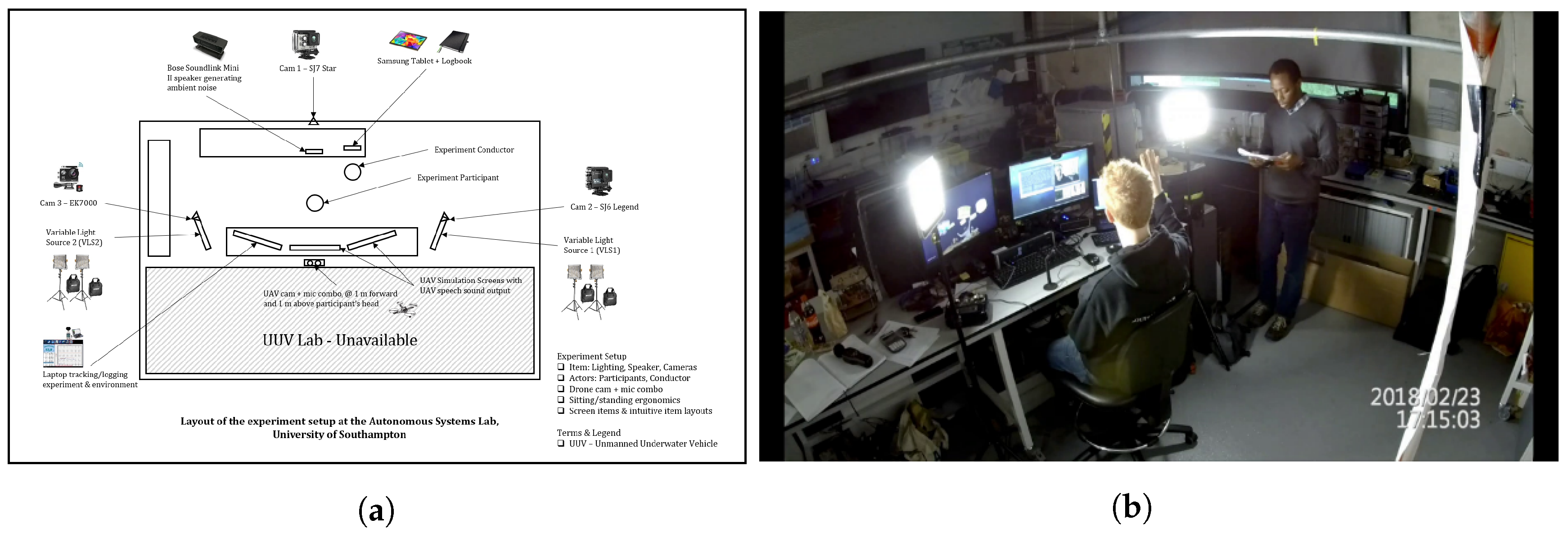
A computer-based hardware-in-the-loop lab experiment was designed with 37 human participants, in order to (1) determine the effect of varying noise levels (55 dB to 85 dB) on speech recognition, and (2) the effect of varying lighting levels (10 Lux to 1400 Lux) using different lighting colour temperature of white (5500 K) and yellow (3500 K), and a mixture of these colour temperatures with different capture backgrounds, on visual gesture recognition. This study builds on the progress from a previous work by [3]. Unlike in the previous work by [3], where only five participants were used in the study, we have recruited 37 participants and have a broader set of data to draw and generalise conclusions from. This work validates and advances the work done in [3] further by performing more in-depth and multi-dimensional analysis on a larger number of subjects. It was observed that, as noise level increases, the speech command recognition rate drops. A regression characteristic model was developed for the custom CMU Sphinx automatic speech recogniser showing speech control command performance for each ambient noise level ranges of 55 dB to 85 dB. The upper limit of the custom developed CMU Sphinx based speech interface was determined to be 75 dB with a 65% recognition rate. Beyond this threshold, speech control was considered not practical due to the significantly high rate of control failure. This limit was well within the practical operation limit of the HoverCam UAV propulsion noise level, but not the DJI Phantom 4 Pro. Some ways of improving this limits were suggested, such as investigating other speech recognisers with a different model other than the hidden Markov model, which was used in this particular study. From the varying lighting experiment, it was clear that background and lighting levels only had a very little effect on gesture quality, and that the gesture capture system and processing methods were more critical to the successful recognition of gesture commands.

2. Literature Review

The ability to interact with aerobots via speech and gesture is useful in areas such as search and rescue [4] and drone delivery [5,6]. The aerobot could be equipped with light sensors, cameras, auditory sensors, and output feedback devices like speakers or a laser projector. Ng [7] observed users combining speech and two hand gestures in communicating control intentions to a UAV in a Wizard of Oz simulation experiment designed to investigate collocated interaction with flying robots. Cauchard and Obaid [8,9] performed an elicitation studies to determine what gestures are considered intuitive for controlling a UAV. Ng, Cauchard, and Abioye [1,2,7,8] considered that speech could be used to augment gesture in human aerobotic interaction. Cauchard [10] investigated a gestural and visual interface for human–drone interaction, with the aid of a mobile projector carried by the aerobot—displaying input options and output information, in an aerial tour guide application of the aerobot. Mohaimenianpour [11] researched real-time robust gesture recognition algorithms that could aid the fast detection of users hands and faces, for practical UAV control applications. Schelle [12,13] also investigated the possibility of visually communicating control to small multi-rotor UAVs via gestures. Visual gesture communication with aerobots could improve intelligence, surveillance and reconnaissance (ISR) missions, redefined how ground personnel control flying transport vessels, aid search and rescue operations as missing persons could attract attention to themselves and increase their chances of being discovered.

Multimodal Speech and Gesture Interfaces

Multimodal speech and gesture interfaces are actively being developed for many mobile and stationary robotic systems. Cacace [14] investigated multimodal speech and gesture communication with multiple UAVs in a search and rescue mission using the Myo armband device. The result of their simulation showed that human operators could interact effectively and reliably with UAVs via multiple modalities of speech and gesture, in autonomous, mixed-initiative, or teleoperation mode. Fernandez [15] investigated the use of natural user interfaces (NUIs) in the control of small UAVs, using a custom Aerostack software framework, which they developed by combining several NUI methods and computer vision techniques. Their project was aimed at studying, implementing, and validating NUIs efficiency in human UAV interaction [15]. Harris and Barber [16,17] investigated the performance of a speech and gesture multimodal interface for a soldier–robot team communication during an ISR mission. They also suggested the possibility of developing complex semantic navigation commands such as “perch over there (speech + pointing gesture), on the tank to the right of the stone monument (speech)” [16,18]. Speech can be used to provide contextual information for the ‘pointing’ gestures and vice versa. In a related research by [19], the researchers suggested that multimodal speech and gesture communication was a means to achieving an enhanced naturalistic communication, reducing workload, and improving the human–robot communication experience. Kattoju [20] also investigated the effectiveness of speech and gesture communication in soldier–robot interaction. Ng [7] investigated collocated interaction with flying robots, studying participants’ behaviour around UAVs. Cauchard and Obaid [8,9] conducted elicitation studies to determine what gestures are considered intuitive for controlling UAVs. Abioye [4] justifies the application of a multimodal speech and visual gesture interface for interacting with patrol, search, and rescue UAVs.

3. Methodology

3.1. Speech Interface

Speech is one component of the proposed mSVG aerobot control interface. In this method, controls are issued via voice commands. A microphone is used to detect the sound wave generated by an operator’s voice commands, which is then converted into an electrical signal for processing. The operator’s speech command may be identified by querying a database of speech command vocabulary with the captured speech signal, for a match. Some popular audio speech recognition (ASR) toolkits are the Microsoft speech platform SDK, CMU PocketSphinx, and Google web speech API (Application Programming Interface) [17]. In order to develop a speech control method for a UAV, one needs to take into account the average noise level generated by the UAV’s multirotor propulsion system, in addition to the ambient noise levels. Islam and Levin [21,22] both conducted an experiment to measure the noise level generated by small UAVs. In [22]’s experiments, five small UAVs were tested by flying the UAVs to a 1 m altitude, and placing a soundmeter 1 m adjacent to the UAV. The results obtained have been summarised in

Table 1. Noise levels generated by some small multirotor unmanned aerial vehicles (UAVs) [22].

S/N	Small Multirotor UAV	Noise Levels (dB)
1	DJI Phantom 2	75.8
2	DJI Phantom 3 Pro	76.3
3	DJI Phantom 4 pro	76.9
4	DJI Inspire 2	79.8
5	Hover Cam	72.1
6	DJI Mavic Pro	∼65
7	DJI Mavic Pro Platinum	∼60

. From this result, and for the purpose of this study, the noise level generated by the small multirotor UAV would be assumed to be approximately 80 decibels. Sound reduces at a rate of 6 dB for every doubling of distance from a noise source [23]. Therefore, if a DJI phantom 2 generates $75.8$ dB of noise at 1 m, then it would be $69.8$ dB at 2 m, 81.8 dB at 0.5 m, and 87.8 dB at 0.25 m. The selection of the noise level range of 55 dB to 85 dB, was based on these practical noise levels generated by real small multirotor UAVs.

3.2. Gesture Interface

The gesture interface is the second component of the mSVG interface. The method used in this work was similar to that described in [24] where hand gestures were recognised with the aid of convexity hall defects [25]. A four-stage image processing operation of skin detection, noise elimination, convex hull and convexity defect processing, was performed with the aid of OpenCV algorithm libraries, in order to count the number of fingers being held up by a human user. In order to isolate the hand gestures from other environmental components in the image, skin colour detection was performed in the $Y^{\prime }{C}_B{C}_R$ colour space. In order to achieve robust skin colour detection under varying illumination conditions, the luminance Y’ was separated from the blue-difference chrominance $C_B$ and red-difference chrominance $C_R$ of the skin. Noise filtering was achieved by using $cvErode(\ast )$ and $cvDilate(\ast )$ OpenCV functions, with the first function eroding/trimming down areas were the hand was not detected, and the second function dilating/enlarging the non-eroded areas for further processing. This process effectively removes noisy pixels from the image. An outline of the hand, from which the convex hull was to be computed, was then generated. This was achieved through the application of an OpenCV function, $cvDrawContours(\ast )$. The $cv2.convexHull(\ast )$ function checks for convexity defects in curves and tries to correct it. Convex curves are usually bulged out, or at least flat. Convexity defect arises where curves bulge inwards. The number of defects and the Euclidian distance of the defects from the geometric centre of the contour was used in determining the number of fingers. Using a similar method [26] developed a convex hull defect based virtual finger pointer and finger counter.

Hand gestures may vary across different usage context, geographical region, and cultural backgrounds. Hand gestures could be specific to particular professional fields such as the military, traffic controllers, airfield assistants, etc. Gestures could also be a language such as the American Sign Language (ASL) and Mexican Sign Language (MSL). However, for the purpose of this study, finger counting gestures (one finger, two fingers, three fingers, four fingers, and five fingers) were used to demonstrate the application of gestures in its simplest form. The gesture complexity would be built upon in future studies.

3.3. Experiment Study Design

For this research’s investigation, a hardware-in-the-loop simulation experiment involving human participants was designed. The experiment was conducted with the aid of a computer-based UAV simulator, augmented with external hardware components: a single-board computer, a web camera, a microphone, a speaker, and two multi-colour (white and yellow) variable LED (Light Emitting Diode) lighting systems, which were laid out as shown in Figure 1a. Unlike typical pure simulation experiments, the hardware-in-the-loop experiment enabled practical interaction with the real world components, making the results more generalisable to practical real world applications.

The study participants were mostly sited in front of a three-screen UAV simulation computer workstation, during which the participant were asked to perform a series of task. The first task measured the effect of varying noise levels from 55 dB to 85 dB in steps of 5 dB, being generated from a Bose Sound link Mini speaker system, playing a pre-recorded loop of a multirotor UAV propeller-rotor noise sound. The second task observed how varying the ambient lighting conditions from 10 Lux to 1400 Lux, for each white, yellow, and mixed lighting condition, against the backdrop of a green, blue, and white solid background surface, affects the quality of the finger gesture recognition. The gesture was processed on an Odroid XU4 single board computer and captured via a webcam device, in the same way it would be setup on a practical UAV. By processing both the speech and gesture control input on a linux based single board computer, such as the Odroid XU4, the mSVG control technique is made portable and easy to plug into other commercial UAV flight controller systems like the PixHawk, having the single board computer convert the high level nCA Tier I-III [2] or higher commands to lower levels that the flight controller can handle.

The experiment participants were asked to repeat a series of 12 speech commands made from a vocabulary of 12 words. The commands were “go forward, go backward, step left, step right, hover, land, go forward half metre, go backward one metre, hover one metre, step left half metre, step right one metre, and stop”. The first six speech commands were selected because they were essential UAV navigation commands that specify fundamental horizontal motion in the x and y coordinate directions at a fixed z altitude/vertical coordinate. The seventh to eleventh commands were randomly selected commands used to emulate practical x, y, and y coordinate navigation were short distance (less than 3 m) modifiers were applied. The twelfth command was selected based on practical consideration for a fail-safe/emergency/urgent command phrase that halts any current motion action. These commands are issued at quiet lab conditions of 55 dB, and then repeated for 60 dB, 65 dB, 70 dB, 75 dB, 80 dB, and 85 dB noisy lab conditions. The results are presented and discussed under Section 4 and Section 5.

For the second part of the experiment on how varying ambient lighting conditions and changing background affects gesture recognition quality, the procedure was to divide the experiment into a sequence of nine lighting stages (LS1–LS9). The default room lighting was turned off, all window blinds closed, and the main lighting source was the LED lamp with two colour LEDs—white (5500 K) and yellow (3500 K), as shown in Figure 1b. For the first light stage, LS1, the LED lamps were turned off and ambient stray light rays from workstation monitors, of around 10 Lux was measured and recorded against each of the solid coloured finger gesture capture background surface area. The green background was setup first, and the user asked to hold up the following finger gestures in order: ‘one finger’, ‘two fingers’, ‘three fingers’, ‘four fingers’, and ‘five fingers’. The background qualities are estimated based on how distinct the finger gestures were clearly recognised using a numeric scale of 1–10, with ‘1’ being a complete failure in gesture recognition, ‘3’ being the hand outline was successfully registered, ‘5’ being all finger gestures being successful but with high frequency noise fluctuations, and ‘7’ being all fingers were clearly distinguished but with small low frequency fluctuations (one in 10 s), and ‘10’ being perfect steady recognition, with no noise fluctuations within 60 s. This was repeated for the blue and white background. Then, the second lighting stage, LS2 experiment was performed, turning only the white lighting knob to the first indicator point on the right LED lamp, and repeating the capture procedure described for LS1. Note that all other knobs were reset to zero. For LS3, the white lighting knob was turned to the first indicator point on both the right and left LED lamps. All of the white knobs’ positions were then reset back to zero before proceeding to LS4. For LS4, the yellow lighting knob was turned to the first indicator point on the right LED lamp. For LS5, the yellow lighting knobs were turned to the first indicator point on both the right and left LED lamp. For LS6, the white and yellow lighting knobs were turned to the first indicator point on both the right and left LED lamps. After completing LS6 capture, the yellow lighting knobs were reset back to zero. For LS7, the white lighting knob was turned to the maximum position on both the right and left LED lamp. After the LS7 capture, all white lighting knobs were reset back to zero. For LS8, the yellow lighting knobs were turned to the maximum position on both the right and left LED lamp. Finally, for LS9, both the white and yellow lighting knobs were turned to the maximum position on both the right and left LED lamps. For each of these LS settings, the capture procedure described for LS1 was repeated. Note that LS2, LS3, and LS7 were the white lighting capture experiment stages. LS4, LS5, and LS8 were the yellow lighting experiment stages. LS1, LS6, and LS9 were the mixed white and yellow lighting experiment stages. The results were presented and discussed in Section 6.

A risk assessment was completed for this study and the study was approved by the University of Southampton Ethics and Research Governance Community with the ethics approval code: 30377. The research dataset is being made available for publication with this submission.

4. Varying Noise Level—Speech Command Results

The varying noise level speech command results from the experiment are recorded in a spreadsheet document, which is made available as downloadable supplementary material/dataset for this research paper. The blanks indicated by an underscore, in the varying noise level speech command result spreadsheet tab, are points were the data was not available due to lab threshold noise levels being higher than specified, caused by uncontrollable ambient noise conditions during experiments. In addition, all of participant A1’s data in this segment were corrupt due to setup failure at the beginning of the experiments. The implication of this is that the total sum of utterances may be fewer than 37, mostly 36 at each noise dB level.

Each of the 12 speech commands were collated across the 37 participants, and the number of words successfully recognised were plotted against the noise levels with the number of times the number of words were recognised for the particular speech command by different participants, which is the hit frequency of each point on the plot was being indicated in brackets. This was called the frequency map. A MATLAB program was written to collate and plot the data from the result table. From the frequency map shown in Figure 2, it can be observed for the two-word speech command “Go Forward” that all of the 23 utterances successfully made at 55 dB were successfully recognised as two-word commands, as indicated in the bracket next to the point on the frequency map plot. In addition, at 60 dB, it can be observed that, of the 35 successfully registered commands, 30 were two-word (full recognition—success), four were one-word (partial recognition—partial success), and one was no-word (recognition failure). The distribution of the partial success is presented in the next section on “variable noise level—word frequency.” At 65 dB, there were 36 commands that were successfully registered/uttered/recorded, but only 27 were two-worded (success), five one-worded (partial success), and four failures (no-word). At 70 dB, 11 were successfully recognised as two-worded, 12 partial success (one-word), and 13 failures (no-word). At 75 dB, there were 36 registered commands, eight two-word success, seven one-word partial success, and 21 failures (no word recognised). At 80 dB, there were 36 registered commands, zero two-word success, six one-word success, and 30 failures (no-word). At 85 dB, 36 registered commands, and 36 failures, no word was recognised at 85 dB by the custom UAV-Speech interface.

A trend can be observed here, that at the lower dB noise level, the two-word speech command “Go Forward” was successfully recognised, whereas recognition fails at higher dB noise levels. This trend is graphically shown by the trendline plot in Figure 3. The points on the trendline were computed by taking the vertical weighted average from the frequency map as follows:

$$y\left(x\right)=\frac{{\sum }_{i=0}^n{d}_i\left(x\right)f_i\left(x\right)}{{\sum }_{i=0}^n{f}_i\left(x\right)},$$

(1)

where $n=4$ is the maximum number of speech command words used in the experiment. $d_i\left(x\right)$ is the specific number of speech command words being registered, for the given x dB noise level. Note that this corresponds to the ith value. $f_i\left(x\right)$ is the frequency of the $d_i\left(x\right)$ point, as indicated on the frequency map, for the given x dB noise level.

For example, the points on the trendline for the first speech command (SC1), “Go Forward” was computed as follows:

When $x=55$ dB

$$y\left(55\right)=\frac{{\sum }_{i=0}^4{d}_i\left(55\right)f_i\left(55\right)}{{\sum }_{i=0}^n{f}_i\left(55\right)}.$$

(2)

$$=\frac{d_0\left(55\right)f_0\left(55\right)+d_1\left(55\right)f_1\left(55\right)+d_2\left(55\right)f_2\left(55\right)+d_3\left(55\right)f_3\left(55\right)+d_4\left(55\right)f_4\left(55\right)}{f_0\left(55\right)+f_1\left(55\right)+f_2\left(55\right)+f_3\left(55\right)+f_4\left(55\right)}.$$

(3)

$$=\frac{0·0+1·0+2·23+3·0+4·0}{0+0+23+0+0}=2.$$

(4)

When $x=60$ dB

$$y\left(60\right)=\frac{{\sum }_{i=0}^4{d}_i\left(60\right)f_i\left(60\right)}{{\sum }_{i=0}^n{f}_i\left(60\right)}.$$

(5)

$$=\frac{d_0\left(60\right)f_0\left(60\right)+d_1\left(60\right)f_1\left(60\right)+d_2\left(60\right)f_2\left(60\right)+d_3\left(60\right)f_3\left(60\right)+d_4\left(60\right)f_4\left(60\right)}{f_0\left(60\right)+f_1\left(60\right)+f_2\left(60\right)+f_3\left(60\right)+f_4\left(60\right)}.$$

(6)

$$=\frac{0·1+1·4+2·30+3·0+4·0}{1+4+30+0+0}=1.8286.$$

(7)

When $x=65$ dB,

$$y\left(65\right)=\frac{{\sum }_{i=0}^4{d}_i\left(65\right)f_i\left(65\right)}{{\sum }_{i=0}^n{f}_i\left(65\right)}=\frac{0·4+1·5+2·27+3·0+4·0}{4+5+27+0+0}=1.6389.$$

(8)

When $x=70$ dB,

$$y\left(70\right)=\frac{{\sum }_{i=0}^4{d}_i\left(70\right)f_i\left(70\right)}{{\sum }_{i=0}^n{f}_i\left(70\right)}=\frac{0·13+1·12+2·11+3·0+4·0}{13+12+11+0+0}=0.9444.$$

(9)

When $x=75$ dB,

$$y\left(75\right)=\frac{{\sum }_{i=0}^4{d}_i\left(75\right)f_i\left(75\right)}{{\sum }_{i=0}^n{f}_i\left(75\right)}=\frac{0·21+1·7+2·8+3·0+4·0}{21+7+8+0+0}=0.6389.$$

(10)

When $x=80$ dB,

$$y\left(80\right)=\frac{{\sum }_{i=0}^4{d}_i\left(80\right)f_i\left(80\right)}{{\sum }_{i=0}^n{f}_i\left(80\right)}=\frac{0·30+1·6+2·0+3·0+4·0}{30+6+0+0+0}=0.1667.$$

(11)

When $x=85$ dB,

$$y\left(85\right)=\frac{{\sum }_{i=0}^4{d}_i\left(85\right)f_i\left(85\right)}{{\sum }_{i=0}^n{f}_i\left(85\right)}=\frac{0·36+1·0+2·0+3·0+4·0}{36+0+0+0+0}=0.$$

(12)

Similarly, the frequency map and trendline of the other 11 speech command phrases are presented in Figure 4, Figure 5 and Figure 6, after performing a similar analysis. Figure 4 shows the results of four speech commands. In particular, Figure 4a,b shows the frequency map and trendline of the second speech command (SC2), “Go Backward”. This is a two-word command which seems to have a slightly better performance across the experiment participants than the first speech command (SC1), “Go Forward”, particularly between 70 dB and 80 dB. Figure 4c,d shows the frequency map and trendline of the third speech command (SC3), “Step Left”, another two-word command. Figure 4e,f shows the frequency map and trendline of the fourth speech command (SC4), “Step Right”, a two-word command which seems to have been the most successful of all the other two-word commands previously presented. SC4 has a recognition accuracy of over 90% at 75 dB and about 70% at 80 dB. Figure 4g,h shows the frequency map and trendline of the fifth speech command (SC5), “Hover”, a one-word command, which had the poorest performance of all the speech command set in the experiment. It performance was observed to be as low as 22% at 65 dB. This was mainly attributed to its subtle articulation, which leaves it easily prone to noise corruption even at low noise levels. In addition, the SC5 failure was also partly attributed to the speech ASR implementation not being robust enough. Commercial or industrial speech ASR interfaces, such as the Amazon Echo, Apple Siri, and Microsoft Cortana, may offer an improved performance due to their use of more advanced and online AI learning algorithms, whereas the custom CMU Sphinx ASR that was used in this application was based on offline hidden Markov models (HMM).

Figure 5 shows the results of four more speech commands, SC6–SC9. Figure 5a,b shows the frequency map and trendline of the sixth speech command (SC6), “Land”, which is also a one-word speech command. However, unlike SC5: Hover, SC6: Land, had a better performance, with recognition accuracy of over 90% at 75 dB and about 67% at 80 dB. Figure 5c,d shows the frequency map and trendline for the seventh speech command (SC7), “Go Forward Half Metre”, which is a four-word command. The result, as presented here, does not give additional information on which of the four words are failing, and whether these are primary keywords, primary modifiers, secondary keywords, or secondary modifiers’ parameters. Note that the failure of the two primary parameter/words could be considered as the failure of the control command. However, a more general approach is used to address this, by investigating the overall word failure frequency in a later section. Figure 5e,f shows the frequency map and trendline for the eighth speech command (SC8), “Go Backward One Metre”, another four-word speech command. Figure 5g,h shows the frequency map and trendline for the ninth speech command (SC9), “Hover One Metre”, a three-word command.

Figure 6 shows the results of the remaining three speech commands, SC10–SC12. Figure 6a,b shows the frequency map and trendline of the tenth speech command (SC10), “Step Left Half Metre”, a four-word speech command with over 75% and about 50% recognition accuracy rate at 75 dB and 80 dB, respectively. Figure 6c,d shows the frequency map and trendline of the eleventh speech command (SC11), “Step Right One Metre”, another four-word speech command. Similar to SC4 “Step Right”, SC11 had a good performance with a recognition accuracy of 92% and 67% at 75 dB and 80 dB, respectively. Both SC4 and SC11 share the same base keywords of “Step Right”, the recognition of which seems to be highly successful in all cases. This would be investigated further when breaking down the speech command constituents, in a later section investigating speech command keyword selection. Figure 6e,f shows the frequency map and trendline of the tenth speech command (SC12), “Stop”, a one-word speech command with 91% and 64% recognition accuracy rate at 75 dB and 80 dB, respectively.

4.1. Speech Command Performance Comparison

In order to compare the performance of each of the 12 speech commands using their trendline characteristic, each weighted trendline was normalised so they can all be plotted on to the same y-axis, overlaid on the same graph and visually compared. This was done by dividing the weighted trendline $y\left(x\right)$ values previously computed by the number of words in the speech command. Mathematically, normalised

$$Y_N\left(x\right)=\frac{Y\left(x\right)}{n}=\frac{1}{n}\left[\begin{array}{ccccccc}y\left(55\right)& y\left(60\right)& y\left(65\right)& y\left(70\right)& y\left(75\right)& y\left(80\right)& y\left(85\right),\end{array}\right]$$

(13)

where n is number of words in the specific speech command being normalised. The resulting comparison plot is as shown in Figure 7. Note that the poorest performance was observed in the speech recognition of SC5, ‘Hover’, followed by SC1 ‘Go Forward’ and SC2 ‘Go Backward’ as indicated in the combined trendline in Figure 7. The best speech recognition performance was observed in SC4 ‘Step Right’, SC6 ‘Land’, SC11 ‘Step Right One Metre’, and SC12 ‘Stop’. Both single-word and multi-word speech commands were found in each performance category. In addition, the fact that significant fail safe commands, such as SC6 ‘land’ and SC12 ‘stop’, were among the most resilient to noise corruption, having a high recognition success rate at a higher noise level, is very important in UAV applications, where fail safe commands are expected to be very reliable; otherwise, it may be impractical to use.

4.2. Experiment SC ASR Characteristic

In order to determine the characteristic curve describing the speech command performance within a UAV type application environment, given the custom CMU Sphinx ASR implementation, and the set of speech control commands, an average of the normalised trendline plotted in Figure 7 is computed and plotted. The average trendline characteristics,

$$y_c\left(x\right)=\frac{y_{N_1}\left(x\right)+y_{N_2}\left(x\right)+\cdots +y_{N_n}\left(x\right)}{n},$$

(14)

$$=\frac{{\sum }_{i=1}^n{y}_{N_i}\left(x\right)}{n},$$

(15)

where $y_{N_i}\left(x\right)$ is the normalised value of y at x dB for the $i_{th}$ speech command. In addition, $n=12$ since there are 12 speech commands in this case. The result is the performance characteristic curve shown in Figure 8a. This curve can be used in predicting the response of the developed speech control interface for the small multirotor UAV, setting the practical limit of the current speech control interface implementation and quantifying the effects of performance modification on the implementation. In addition, other speech control methods that uses other ASR engines with different underlying theory other than Hidden Markov Model (HMM) as is the case with the CMU Sphinx, such as Amazon Echo, Microsoft Cortana, and Apple Siri, could be effectively compared with this implementation using the characteristic performance curve. However, unlike many of the alternatives, the current implementation is low-cost and works offline without relying on network connectivity to function effectively.

4.3. Characteristic Curve Fitting

In order to make the UAV speech command interface performance characteristic easily exportable for other application purposes, the curve was fitted to a polynomial line with three degrees of freedom,

$$y=a{x}^3+b{x}^2+cx+d,$$

(16)

where $a=-0.00005147$, $b=0.00965375$, $c=-0.61458338$, and $d=14.15673367$, then

$$y=-0.00005147x^3+0.00965375x^2-0.61458338x+14.15673367,x\in \Re \mid 55\le x\le 85.$$

(17)

The degrees of freedom were considered sufficient as polynomials with higher degree of freedom values had coefficients that were near zero (≪10${}^{-4}$). In addition, higher degree of freedom values risk characteristic curve over-fitting. In addition, because of the nature of the curve, other curve fittings such as linear or exponential were considered unsuitable. The curve fit was generated using MATLAB. The resulting line of best fit equation presented in Equation (17), was plotted over the curve generated in Figure 8a to give the characteristic curves shown in Figure 8b. The original characteristic curve is the black solid line in the plot, while the fitted characteristic curve is the red dash-dot line.

5. Varying Noise Level—Word Frequency Results

In this section, the experiment results were analysed based on the individual word frequency rather than the speech command phrase as performed in Section 4. There are a total of twelve $\left(12\right)$ unique words that make up the twelve $\left(12\right)$ UAV speech command phrases. Similar to the speech command phrase analysis in the previous section, the total number of each of the 12 words (contained in the 12 speech command phrases) that were successfully recognised were collated across the 37 participants. For each word, a frequency map and a trendline plot was generated as presented in Figure 9, Figure 10 and Figure 11.

The frequency map is a plot of the total number of times (zero, one, two, three, four, and five) each word was recorded across all participants for each noise level. For example, Figure 9a shows the observation for the first speech word (SW1) ‘Go’ which appeared a total of four times across all 12 speech command phrases. At 55 dB, of the twenty-three participants whose data were successfully captured and processed, twenty-one had all 4 of the 4 ‘Go’ word instances successful, one had 3 out of 4 successes, and another one had 2 out of 4 successes. At 60 dB, 4 out of 4 ‘Go’ word results were successfully recorded for twenty-five participants, 3 out of 4 for five participants, 2 out of 4 for two participants, 1 out of 4 for two participants, and 0 out of 4 for one participant. At 65 dB, of the 36 participants successfully captured and processed, the 4 of 4 ‘Go’ word recognition was successful for 21 participants, 3 out of 4 for three participants, 2 out of 4 for four participants, 1 out of 4 for two participants, and 0 out of 4 for six participants. At 70 dB, the 4 of 4 ‘Go’ word recognition was thirteen times, 3 out of 4 was one time, 2 out of 4 was one time, 1 out of 4 was five times, and 0 out of 4 was sixteen times. At 75 dB, the 4 of 4 ‘Go’ word recognition was seven times, 3 out of 4 was three times, 2 out of 4 was one time, 1 out of 4 was five times, and 0 out of 4 was sixteen times. At 80 dB, the 4 of 4 ‘Go’ word recognition was two times, 3 out of 4 was two times, 2 out of 4 was five times, 1 out of 4 was two times, and 0 out of 4 was twenty-five times. At 85 dB, the 4 of 4 ‘Go’ word recognition was zero, 3 out of 4 was zero, 2 out of 4 was zero, 1 out of 4 was zero, and 0 out of 4 was thirty-six times. From this result, a decrease can be observed in the total number of times each word was recognised as the noise level was increased from 55 dB to 85 dB. This was represented by the trendline shown in Figure 9b, which was computed using a similar equation to the weighted trendline Equation (1) in the speech command analysis,

$$y\left(x\right)=\frac{{\sum }_{i=0}^n{d}_i\left(x\right)f_i\left(x\right)}{{\sum }_{i=0}^n{f}_i\left(x\right)},$$

(18)

where n is the total number of each word presented in the 12 speech commands combined, as used in the experiment. Note that n is different for each word, for example $n=4$ for SW1 ‘Go’, $n=2$ for SW2 ‘Forward’, $n=1$ for SW8 ‘Land’, $n=3$ for SW10 ‘One’, and $n=5$ for SW11 ‘Metre’. $d_i\left(x\right)$ is a coefficient less than or equal to n specifying the number of recognition out of n word repetitions in a total set of 12 speech commands, for the given x dB noise level. Note that this corresponds to the ith value. $f_i\left(x\right)$ is the frequency (number of times) of the $d_i\left(x\right)$ of n recognition for the given word at the given x dB noise level, as indicated on the frequency map.

For example, the points on the trendline for the first speech word (SW1), ‘Go’ was computed and yielded the following values: $y\left(55\right)=3.8696$, $y\left(60\right)=3.4571$, $y\left(65\right)=2.8611$, $y\left(70\right)=1.7222$, $y\left(75\right)=1.1667$, $y\left(80\right)=0.7222$, and $y\left(85\right)=0$.

Figure 9c,d shows the frequency map and trendline of the second speech word (SW2), ‘Forward’, which appeared only two times in the 12 speech command set. Observe that about half of this command word fails at 70 dB, which is poor for a key command word for which a higher resilience is needed at higher levels of 75 dB and perhaps 80 dB. Figure 9e,f shows the frequency map and trendline of the third speech word (SW3), ‘Backward’, which appeared only two times in the 12 speech command set. It had a better performance than SW2, notably at both 75 dB and 80 dB. Figure 9g,h shows the frequency map and trendline of the fourth speech word (SW4), ‘Right’, which also appeared only two times in the 12 speech command set, was the most noise resilient and hence the most successful speech command word with a high recognition accuracy of about 90% at 80 dB.

Figure 10 shows the results of four speech words, SW5–SW8. Figure 10a,b shows the frequency map and trendline of the fifth speech word (SW5), ‘Left’, which appears twice in the 12 speech command set. Figure 10c,d shows the frequency map and trendline for the sixth speech word (SW6), ‘Step’, which appears four times in the 12 speech command set. Figure 10e,f shows the frequency map and trendline for the seventh speech word (SW7), ‘Hover’, which appears twice in the 12 speech command set. This was the least successfully recognised speech command word across all participants, with a recognition rate of 36 % at 65 dB. Figure 10g,h shows the frequency map and trendline for the eighth speech word (SW8), ‘Land’, which appeared only once in the 12 speech command set. Note that this has exactly the same frequency map and trendline characteristic as speech command SC6 ‘Land’ in Figure 5a,b because it is a single word command that appears only once in the speech command set, therefore both speech command and individual word dimensions of analysis yield the same result.

Figure 11 shows the results of the remaining four speech words, SW9–SW12. Figure 11a,b shows the frequency map and trendline of the ninth speech word (SW9), ‘Half’, which appears twice in the 12 speech command set. Figure 11c,d shows the frequency map and trendline for the tenth speech word (SW10), ‘One’, which appears three times in the 12 speech command set. Figure 11e,f shows the frequency map and trendline for the eleventh speech word (SW11), ‘Metre’, which appears five times in the 12 speech command set. This had the highest frequency of occurrence because it is a modifier specifying the unit of movement in any direction being given by the keyword. Figure 11g,h shows the frequency map and trendline for the twelfth speech word (SW12), ‘Stop’, which appeared only once in the 12 speech command set. This has exactly the same frequency map and trendline characteristic as speech command SC12 ‘Stop’ in Figure 6e,f because it is a single word command that appears only once in the speech command set; therefore, both speech command and individual word dimensions of analysis yield the same result.

5.1. Speech Word Performance Comparison

The performance of each of the speech word was compared using the same method described in Section 4.1 with the aid of Equation (13). The resulting comparison plot is shown in Figure 12. Note that the poorest performance was observed in the speech word recognition of SW7, ‘Hover’, followed by SW2 ‘Forward’ and SW1 ‘Go’ as indicated in the combined trendline in Figure 12. The best speech recognition performance was observed in SW4 ‘Right’, SW8 ‘Land’, SW10 ‘One’, SW11 ‘Metre’, and SW12 ‘Stop’.

5.2. Experiment SW ASR Characteristic

Similar to the SC ASR Characteristic curve presented in Section 4.2, the average of the normalised trendline plotted in Figure 12 is computed and plotted to give the SW ASR Characteristic shown in Figure 13a, which was computed with the aid of Equation (15).

5.3. SW Characteristic Curve Fitting

Fitting the SW ASR characteristic curve to a three degree of freedom polynomial curve of the form,

$$y=a{x}^3+b{x}^2+cx+d,$$

(19)

where $a=-0.00004949$, $b=0.00916273$, $c=-0.57521151$, and $d=13.14811872$, yielded

$$y=-0.00004949x^3+0.00916273x^2-0.57521151x+13.14811872,x\in \Re \mid 55\le x\le 85.$$

(20)

This is plotted as shown in Figure 13b, where the original characteristic curve is the black solid line in the plot, and the fitted characteristic curve is the red dash-dot line.

6. Varying Lighting Level Results

This section presents the result from the varying lighting level (VLL) experiments. The complete result from this segment of the experiment is included in the downloadable supplementary material for this paper. The results consisted of about 999 gesture observations, from nine lighting stages, three background quality experiment per stage, and 37 experiment participants. The blanks indicated by an underscore are points where the data were not available due to later improvement in experimental conditions after preliminary testing. For example, the blue and green background were not used during preliminary testing (participants 1–5) but were then made available for the significant remainder of the test (participants 6–37). In addition, all of the participant A10’s data in this segment could not be captured because the equipment calibration failed for the participant. The implication of this is that the total number of observations for all participants for most of the lighting stage parameters is 36, and 31 for the green and blue background parameter. In addition, although the same variable knob settings was used for all participants, slighting different lighting level values were measured up to a span of around 200 lux at higher lighting levels, which also accounts for the scatter observed in the plots. This was due to (1) stray light rays from corridors due to people and lab equipment movements, (2) weather-dependent daylight level penetration via shut windows, and (3) reflection from workstation computer monitors and screens within the experiment lab. However, this was not a problem for the result analysis, since the aim is to observe the quality trend from low to high intensity on different lighting backgrounds and with different lighting sources. They were considered as white noise whose persistent presence throughout the experiment evenly cancels out their effect eventually. For analysis where the scatter could be a problem, the mean lighting level value could be computed across all participants and use as the lighting stage lighting level value. Figure 14 shows the result of room temperature variation for each participants as they progress through different lighting levels going from lighting stage 1 (LS1) to lighting stage 9 (LS9), and it helps validate the fact that the slight differences in the lighting level for each participants does not affect the general trend of rising temperature during the experiment.

Figure 14a is a scatter plot of the room temperature against lighting level during the experiment progression through the lighting stages. The scatter plot has been colour-coded to collate lighting level reading at the same lighting stage together. In Figure 14b, a line of best fit was drawn over the scatter plot data in Figure 14a, using MATLAB. It can be observed from Figure 14b that temperature was gradually rising during the course of the experiment, at a gradient of $a=0.00040479$, given that the equation of the line is

$$y=ax+b=0.00040479x+23.58151862.$$

(21)

There are nine lighting stages (LS1–LS9). At each lighting stage, each of the different background qualities are estimated based on how distinct the finger gestures were clearly recognised using a numeric scale of 1–10, with ‘1’ being a complete failure in gesture recognition, ‘3’ being the hand outline was successfully registered, ‘5’ being all finger gestures being successful but with high frequency noise fluctuations, and ‘7’ being all fingers were clearly distinguished but with small low frequency fluctuations (one in 10 s), and ‘10’ being perfect steady recognition, with no noise fluctuations within 60 s. The results from the varying light level experiment would be presented in three sections according to the incident lighting colour of white, yellow, and mixed.

6.1. White Lighting on Different Background

Figure 15 shows the result of the varying lighting level experiment when only the white LED lighting was used on the different backgrounds. These were the lighting stages 2, 3 and 7 (LS2, LS3, and LS7) steps of the experiment. Figure 15a shows the scatter plot of the result of the finger gesture recognition quality on the green background against the white LED lighting level in Lux (luminous flux incident on the background surface per unit-area/square-metre). Figure 15b shows the line of best fit for the scatter plot shown in Figure 15a. The equation of the line of best fit was $y=0.00101495x+3.37095643$ with a gradient of about $0.10\%$. Figure 15c shows the scatter plot of the result of the finger gesture recognition quality on the blue background against the white LED lighting level in Lux. Figure 15d shows the line of best fit for the scatter plot shown in Figure 15c. The equation of the line of best fit in Figure 15d was $y=0.00186688x+4.25523286$ with a gradient of about $0.19\%$. Figure 15e shows the scatter plot of the result of the finger gesture recognition quality on the white background against the white LED lighting level in Lux. Figure 15f shows the line of best fit for the scatter plot shown in Figure 15e. The equation of the line of best fit in Figure 15f was $y=0.00049768x+5.38390575$ with a gradient of about $0.05\%$.

6.2. Yellow Lighting on Different Backgrounds

Figure 16 shows the result of the varying lighting level experiment when only the yellow LED lighting was used on the different backgrounds. These were the lighting stages 4, 5 and 8 (LS4, LS5, and LS8) steps of the experiment. Figure 16a shows the scatter plot of the result of the finger gesture recognition quality on the green background against the yellow LED lighting level in Lux. Figure 16b shows the line of best fit for the scatter plot shown in Figure 16a. The equation of the line of best fit was $y=0.00335540x+3.17575769$ with a gradient of about $0.34\%$. Figure 16c shows the scatter plot of the result of the finger gesture recognition quality on the blue background against the yellow LED lighting level in Lux. Figure 16d shows the line of best fit for the scatter plot shown in Figure 16c. The equation of the line of best fit in Figure 16d was $y=0.00296837x+3.93542753$ with a gradient of about $0.30\%$. Figure 16e shows the scatter plot of the result of the finger gesture recognition quality on the white background against the yellow LED lighting level in Lux. Figure 16f shows the line of best fit for the scatter plot shown in Figure 16e. The equation of the line of best fit in Figure 16f was $y=0.00035590x+4.32313692$ with a gradient of about $0.04\%$.

6.3. Mixed White and Yellow Lighting on Different Backgrounds

Figure 17 shows the result of the varying lighting level experiment when the white and yellow LED lighting were combined on the different backgrounds. These were the lighting stages 1, 6 and 9 (LS1, LS6, and LS9) steps of the experiment. Figure 17a shows the scatter plot of the result of the finger gesture recognition quality on the green background against the mixed white and yellow LED lighting level in Lux. Figure 17b shows the line of best fit for the scatter plot shown in Figure 17a. The equation of the line of best fit was $y=0.00119177x+3.30883877$ with a gradient of about $0.12\%$. Figure 17c shows the scatter plot of the result of the finger gesture recognition quality on the blue background against the mixed white and yellow LED lighting level in Lux. Figure 17d shows the line of best fit for the scatter plot shown in Figure 17c. The equation of the line of best fit in Figure 17d was $y=0.00192255x+3.99397086$ with a gradient of about $0.19\%$. Figure 17e shows the scatter plot of the result of the finger gesture recognition quality on the white background against the mixed white and yellow LED lighting level in Lux. Figure 17f shows the line of best fit for the scatter plot shown in Figure 17e. The equation of the line of best fit in Figure 17f was $y=0.00156143x+3.58726852$ with a gradient of about $0.16\%$.

7. Discussion

7.1. Speech Command Phrase

The results of the experiment show that speech recognition accuracy/success rate falls as noise levels rise. A regression model was developed from the empirical observation of nearly 3108 speech command utterances—which is 12 speech commands, repeated for each of seven noise levels, by 37 different experiment participants. The polynomial curve fitting characteristic generated for the custom CMU Sphinx ASR can be used to predict speech recognition performance for aerial robotic systems where the CMU Sphinx ASR engine is being used, as well as in the performance comparison with other ASR engines. In addition, it was not clear how the length of speech (the number of speech words in phrase) affects the recognition accuracy because, while there is evidence supporting single-word poor performance like ‘hover’, there is alternative evidence supporting single-word good performance for words like ‘land’ and ‘stop’, in the experiment. However, multi-word speech commands may be more reliable and effective than single-word commands due to the possibility of introducing a syntax error checking stage in the recognition process to validate the control command. The composition of multi-word speech commands consists of keywords and modifiers. For example, in the SC7 command “Go Forward Half Metre”, the primary keyword is ‘Forward’, the secondary keyword is ‘Go’, the primary modifier is ‘Half’, and the secondary modifier is the unit ‘Metre’. In multi-word speech commands, the primary keyword and the primary modifier is the most significant, as the failure of these primary parameters would result in the command execution failure. Secondary modifiers aid system usability particularly for human operators, and could be used for error checking within the UAV system to ensure fidelity of command communication.

7.2. Speech Command Word

From the results of the experiments, it was observed that speech command selection affects the speech recognition accuracy, as some speech command words were found to be more resilient to corruption at higher noise levels, maintaining over 90% success rate at 75 dB, whereas the average rate at 75 dB was just over 65%. In order words, the success of speech command words such as SW4 ‘right’, SW8 ‘land’, and SW12 ‘stop’, at higher noise levels, suggests that some speech command words are more noise resistant than others and that a careful selection of these as part of the speech command phrase could improve the robustness and accuracy of speech recognition in spite of high noise levels, thereby contributing to a more successful human aerobotic speech control interaction.

7.3. Aerobot Speech Interaction

Figure 18 shows the comparison of the speech word (SW) and speech command (SC) trendline characteristic curve. The red solid line represents the SC curve while the black dash-dot line represents the SW curve. Observe that the two curve trends are very similar with the SW curve being below the SC curve, although the SW curve seems to be a replica of the SC curve. The result of the characteristic curve comparison suggests that the speech command phrase slightly outperforms the speech command word, thereby supporting the argument in favour of multi-word commands over single-word commands.

Based on this analysis and the observations in this research, it is recommended that the upper limit of 75 dB noise application level should be set for practical aerobot speech interaction. This was because, at 75 dB, the speech recognition accuracy/success was about 65%, falling below average at 80 dB, and below 5% at 85 dB. In order words, speech is not an effective means of control interaction with an aerobot beyond 75 dB noise level, as the speech control interaction becomes very unreliable due to poor recognition. However, based on the typical UAV noise level data presented in Table 1, it is clear that this limit is below the application range of most small multirotor UAVs. Therefore, there is a need to push the upper limit beyond 75 dB to atleast 80 dB or more. Therefore, the following suggestions are given in order to improve the aerobot speech application:

• Alternative ASR engine: Consider the use of alternative speech ASR technology with a different learning model from the CMU Sphinx’s hidden Markov model, such as artificial neural network or deep learning, for improved noise performance,
• Low noise design: Improve small multirotor UAV propulsion system design to be low noise,
• Application environment: Deploy application only in sub-75 dB noise conditions,
• Speech capture hardware: Consider the use of directional, noise canceling, or array microphones,
• Speech command selection: Optimise the selection of multi-word and single-word speech command in favour of more resilient command variant, as observed in this particular study.

In [3], a previous work, it was observed that ambient noise level above 80 dB significantly affected speech capture. While this conclusion still holds true for the current research work, the current research work had more experiment data to analyse in order to more precisely determine the practical application limits, as presented in this section.

7.4. Lighting Level and Background Effect on Gesture Recognition Quality

The white lighting experiment emulates outdoor daylight at 5500 K colour temperature, while the yellow and mixed lighting experiments emulates indoor lighting conditions of 3500–5500 K colour temperatures. The idea is to consider the aerobot gesture application in both indoor and outdoor (field application) environments. From the varying lighting level experiment results, it was observed that there was only a little improvement in the quality of gesture recognition going from lower light levels to higher lighting levels, as indicated by the gradients from the lines of best fit. Low gradient implies low gesture performance improvement over increasing Lux lighting levels. This observation was consistent across all lighting source (white, yellow, and mixed) and for all three backgrounds of green, blue, and white. The line gradients indicated how much the recognition quality improved from low lighting to higher lighting level, while the intercept indicated the minimum quality threshold. For the white lighting experiment, the blue background had the best improvement with a gradient of 0.19% while the white background had the better minimum quality threshold of 5.38, which means that the finger gestures were clearly recognised but with high frequency noise fluctuations. The green background had the poorest performance. For the yellow lighting experiment, the green background had the best improvement with a gradient of 0.34% while the white background had the better minimum quality threshold of 4.32, which means that the finger gestures were barely distinctly recognised. However, the blue background had the better balance combination of gradient and intercept of 0.30% and 3.94. For the mixed white and yellow lighting experiment, the blue background had the best performance with the best improvement gradient of 0.19% and the best minimum quality threshold of 3.99. The green and white background were similar in their performance.

From these results, the effects of both lighting conditions and the environment background on the quality of gesture recognition were almost insignificant, less than 0.5%. Therefore, other factors, such as the gesture capture system design and technology (camera and computer hardware), type of gesture being captured (upper body, whole body, hand, fingers, or facial gestures), and the image processing technique (gesture classification algorithms) are more important in successfully recognising gesture commands. However, the setup of the gesture capture system and the recognition processing system would still need to take into account the application environmental conditions in order to develop an optimum gesture command interface.

8. Conclusions

In this paper’s investigation of the effects of varying noise levels and varying lighting levels on speech and gesture control command interfaces for aerobots, a custom multimodal speech and visual gesture interface were developed using CMU sphinx and OpenCV libraries, respectively. An experiment was then conducted with 37 participants, who were asked to repeat a series of 12 UAV applicable commands at different UAV propulsion/ambient noise levels, varied in step-sized increase of 5 dB from 55 dB to 85 dB, for the first part of the experiments. For the second part of the experiment, the participants were asked to form finger counting gestures from one to five, under different lighting level conditions from 10 Lux to 1400 Lux, lighting colour temperatures of white (5500 K), yellow (3500 K), and mixed, and on different backgrounds of green, blue, and white, and the quality of the gesture formed was rated on a scale of 1–10. The results of the experiment were presented, from which it was observed that speech recognition accuracy/success rate falls as noise levels rise. A regression model was developed from the empirical observation of nearly 3108 speech command utterances by 37 participants. Multi-word speech commands with primary and secondary modifier parameters were thought to be more reliable and effective than single-word commands due to the possibility of syntax error checking. In addition, it was observed that some speech command words were more noise resistant than others, even at higher noise levels, and that a careful selection of these as part of the speech command phrase could improve the robustness and accuracy of speech recognition at such high noise levels. Speech, based on the custom CMU Sphinx ASR system developed, is not an effective means of control interaction with an aerobot beyond 75 dB noise level, as the speech control interaction becomes very unreliable due to poor recognition. There is a need to push the upper limit beyond 75 dB to at least 80 dB or more, based on current UAV noise ratings (Table 1). Suggestions were made on how to push this limit. From the results of the gesture-lighting experiment, the effects of both lighting conditions and the environment background on the quality of gesture recognition were almost insignificant, less than 0.5%, which means that other factors such as the gesture capture system design and technology (camera and computer hardware), type of gesture being captured (upper body, whole body, hand, fingers, or facial gestures), and the image processing technique (gesture classification algorithms), are more important in developing a successful gesture recognition system.

Further Works

In order to improve the application limit of the aerobot speech interface, alternative automatic speech recognisers with different learning models from the CMU Sphinx’s hidden Markov model would be considered next. ASRs based on artificial neural network or deep learning are of particular interests, such as the IBM Watson speech to text cloud AI service [27]. A hardware upgrade to directional, noise canceling, and array microphones would be considered. Multi and single word speech command selection would be optimised in favour of the more resilient command variant as observed in this particular study.

In order to improve the gesture performance, better alternative hardware (cameras and single board computers) capable of capturing high resolution images and performing complex graphic computation processing in real time would be used. In addition, instead of the appearance-based 2D-model algorithm used in this paper, a more advanced 3D-model based AI gesture algorithm would be developed for capturing and recognising hand, arm, and upper body gestures.