Weightage Effect during Back-Calculation of Rock-Mass Quality from the Installed Tunnel Support in Rock-Mass Rating and Tunneling Quality Index System

Abstract

In extensively used empirical rock-mass classification systems, the rock-mass rating (RMR) and tunneling quality index (Q) system, rock-mass quality, and tunnel span are used for the selection of rock bolt length and spacing and shotcrete thickness. In both systems, the rock bolt spacing and shotcrete thickness selection are based on the same principle, which is used for the back-calculation of the rock-mass quality. For back-calculation, there is no criterion for the selection of rock-bolt-spacing-based rock-mass quality weightage and shotcrete thickness along with tunnel-span-based rock-mass quality weightage. To determine this weightage effect during the back-calculation, five weightage cases are selected, explained through example, and applied using published data. In the RMR system, the weightage effect is expressed in terms of the difference between the calculated and back-calculated rock-mass quality in the two versions of RMR. In the Q system, the weightage effect is presented in plots of stress reduction factor versus relative block size. The results show that the weightage effect during back-calculation not only depends on the difference in rock-bolt-spacing-based rock-mass quality and shotcrete along with tunnel-span-based rock-mass quality, but also on their corresponding values.

1. Introduction

The depth of underground excavations is increasing day by day for different civil and mining engineering projects posing more challenges for safe and economic construction [1,2,3]. The difficulties for modelling such underground excavations due to the complex nature of rock mass are decreasing due to advancement in the research and technology, materials and systems not only in the conventional excavations methods, but also in mechanized one [4,5,6,7]. In underground excavations, the issues related to the rock-mass behavior comprise the strength properties of intact rock, joint related aspects, environmental features (ground water and in situ stresses), configuration of the excavation cross section, and the excavation method; furthermore, these issues define the support required for the underground excavation [8,9]. The ability to forecast the rock-mass quality and support pattern during the design of underground excavation is a challenging and risky task [10]. To stabilize these excavations, researchers characterize the ground in such a manner that is suitable for the support design based on past experiences, which has resulted in the development of different empirical rock-mass classification systems. Till date, empirical rock-mass classification systems have been proposed for the tunnel support system design since the earliest empirical classification proposed by Terzaghi in 1946 known as the rock load classification [4]. Some of the recommended classification systems are not favored by engineers owing to their non-practical application, but few have been frequently used owing to their reliability and practicality. The most extensively used empirical classifications of rock mass during tunnel design and construction in the world are the rock-mass rating (RMR) classifications and tunneling quality index (Q) systems [11,12]. These two systems for the classification of rock masses used by engineers provide convenience in defining the preliminary support systems. The applicability of these systems has been extended with improvements in tunnel construction technology and these systems are revised extensively either in the form of characterization or support [4].

Based on ground behaviors and the available tools for underground excavation in rock engineering, the application of empirical classification systems are limited to different ground behavior during tunnel excavation and stabilization [8]. In empirical classification systems, fiber-reinforced shotcrete and rock bolts are preliminary supports that are recommended during tunnel design and construction, and RMR and Q systems are effective tools for this purpose. The updated versions of these two systems suggest the shotcrete thickness and rock bolt spacing based on the same principles [13], as the excavation support ratio (ESR) in the Q system is not a parameter that is generally used worldwide, and individual countries have their own respective standards [14]. According to these principles, the fiber-reinforced shotcrete thickness is a function of the rock-mass quality (RMR and Q) and tunnel span; however, the rock bolt spacing is only a function of the rock-mass quality. 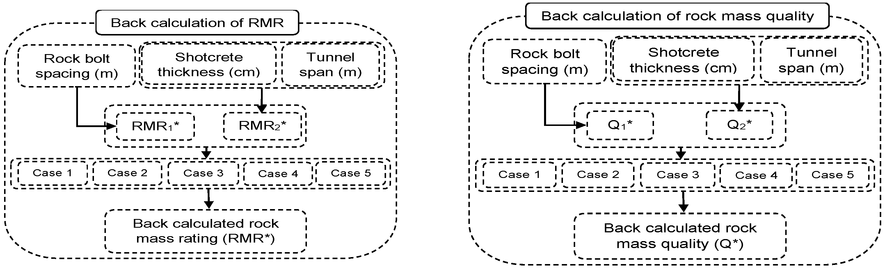During tunnel stability, fiber-reinforced shotcrete and installed rock bolts act as a compound support system and the contribution of individual support depends upon its installation time and distance from the excavation face [15]. Based on the relationships of the rock-mass quality with the spacing of rock bolts (20 mm dimeter) and thickness of fiber-reinforced shotcrete in the support charts of each system, a back analysis approach was established for the determination of the rock-mass quality from the tunnel span, shotcrete thickness, and rock bolt spacing in already supported tunnels [16]. These two relations were used for the back-calculation of the rock-mass quality, and their averaged value (rock-mass quality obtained from shotcrete thickness and tunnel span, and the rock-mass quality obtained from rock bolts spacing) was used for the final calculation of the RMR* (RMR calculated through back-calculation) and Q* (Q value calculated through back-calculation). This averaged value approach is adopted owing to the unavailability of assessment criterion for calculating the rock-mass quality value according to the importance of the support (rock bolt and shotcrete) with the span in the two classification systems.

To extend the application of empirical classification systems (especially RMR and Q) to different ground behaviors for the tunnel excavation and stability, weightage effect during back-calculation of rock-mass quality is critical. Owing to the unavailability criterion for the final calculations of the rock-mass quality (RMR* and Q*), five different cases are taken into consideration in this study to evaluate the weightage effect during the back-calculation of the RMR* and Q*. The weightage adopted in Cases 1 and 3 are already considered for the back-calculation of the rock-mass quality in the Q system for their extension to a highly stressed jointed rock mass [16,17]. However, in the case of RMR₈₉ [18] and RMR₁₄ [19], which are the two versions of the RMR systems, only the Case 3 weightage was assumed in the rock-mass quality back-calculation for the purpose of their extension. The different assessment cases adopted in this study are plotted, and the effect of the weightage in each case is discussed.

2. Materials and Methods

2.1. RMR Classification System and Tunnel Support Design

As established empirically for the tunnel support design by Z. T. Richard Bieniawski in 1973, the RMR classification, also known the geomechanics classification, has been restructured since its establishment, either in its characterization or recommended support pattern or both [11,16,18,19,20,21,22,23,24]. The revised characterization criteria in different version of RMR is shown in

Table 1. Characterization criteria in different versions of the rock-mass rating (RMR) system.

Parameter		RMR
		1973 [11]	1974 [20]	1975 [21]	1979 [22]	1989 [18]	2011 [23]	2013 [24]	2014 [19]
Intact rock strength (MPa)		10–0	10–0	15–0	15–0	15–0	15–0	15–0	15–0
RQD (%)		16–3	20–3	20–3	20–3	20–3	20–0	-	-
Joint spacing (mm)		30–5	30–5	30–5	20–5	20–5	20–0	-	-
Discontinuity density (joints per meter)		-	-	-	-	-	-	40–0	40–0
Separation of joints (mm)		5–1	-	-	-	-	-	-	-
Continuity of joints (m)		5–0	-	-	-	-	-	-	-
Weathering		9–1	-	-	-	-	-	-	-
Condition of joints		-	15–0	25–0	30–0	30–0	30–0	30–0	20–0
Groundwater		10–2	10–2	10–0	15–0	15–0	15–0	15–0	15–0
Alterability (%)		-	-	-	-	-	-	-	10–0
Adjustment	F0	15–3	15–3	0– (−12)	0– (−12)	0– (−12)	0– (−12)	0– (−12)	0– (−12)
	Fe	-	-	-	-	-	-	-	1.32–1
	Fs	-	-	-	-	-	-	-	1.3–1

[4]. The RMR₈₉, which is the 1989 form of the RMR, is still used as a design tool in rock mechanics, particularly for the classification of a rock mass during tunnel support design; furthermore, its latest version is 2014, which is known as RMR₁₄. As a function of six parameters (R₁–R₆), the RMR₈₉ is defined in Equation (1). These six parameters represent the rating for the intact rock uniaxial compressive strength (σ_c), rock quality designation (RQD), spacing of joints (χ), condition of these joints, groundwater condition, and relation of tunnel orientation with respect to joint orientation, respectively.

$$RM{R}_{89}=R_1+R_2+R_3+R_4+R_5+R_6$$

(1)

R₁–R₃ in Equation (1) can be calculated from Equations (2)–(4), respectively [13];

$$R_1=0.126{\sigma }_c-0.0004{\sigma }_c^2, ({\sigma }_{\mathrm{c}}\le 110 \mathrm{MPa}),$$

(2a)

$$R_1=0.475{\sigma }_c^{0.626}, ({\sigma }_{\mathrm{c}}\ge 110 \mathrm{MPa}),$$

(2b)

$$R_2=0.22RQD-0.0002RQ{D}^2,$$

(3)

$$R_3=2.281\times \ln (x)-3.41, (x=5–200 \mathrm{mm});$$

(4a)

$$R_3=4.175\times \ln (x)-13.51, (x=200–900 \mathrm{mm});$$

(4b)

$$R_3=6.250\times \ln (x)-27.55, (x=900–2000 \mathrm{mm}).$$

(4c)

In 2014, a revised structure was proposed for the RMR value calculation with some new parameters, as shown in Equation (5), where RMR_b is the basic RMR; F₀ is a parameter similar to R₆ in Equation (1); and F_s and F_e are parameters that show the effect of the tunnel excavation method and stress–strain behavior at the tunnel face during their construction [19].

$$RM{R}_{14}=(RM{R}_b+F_0)\times F_s\times F_e$$

(5)

RMR_b, F_e, and F_s in Equation (5) can be calculated using Equations (6)–(8), respectively:

$$RM{R}_b=R_1+R_{2–3}+R_4+R_5+R_I$$

(6)

$$F_e=1+2.{\left(\frac{RMR}{100}\right)}^2,\hspace{1em}RMR<40;$$

(7a)

$$F_e=1.32-\frac{\sqrt{(RMR-40)}}{25}, RMR>40$$

(7b)

$$F_s=1.3, ICE<15;$$

(8a)

$$F_s=\frac{2.3\times \sqrt{100-ICE}}{7.1+\sqrt{100-ICE}}, 15<\mathrm{ICE}<70,$$

(8b)

$$F_s=1, ICE>70$$

(8c)

The parameters R_2–3 and R_I in Equation (6) are the ratings for the joint frequency and intact rock alterability. The joint frequency (λ) rating can be calculated using Equation (9). In Equation (8), ICE is the abbreviation of a Spanish word Índice de Comportamiento Elástico, which means index of elastic behavior, and this ICE is the function of the intact rock strength, in situ stresses, rock-mass quality, and tunnel shape and can be calculated using Equation (10) [25].

$$R_{2–3}=34.442\times e^{-0.046\times \lambda }, (\lambda \le 20);$$

(9a)

$$R_{2–3}=22.8-0.457\times \lambda , (\lambda \ge 20).$$

(9b)

$$ICE=\frac{3704\times {\sigma }_c\times e^{\frac{RMR-100}{24}}}{(3-K_0)\times H}\times F, (K_0\le 1);$$

(10a)

$$ICE=\frac{3704\times {\sigma }_{ci}\times e^{\frac{RMR-100}{24}}}{(3\times K_0-1)\times H}\times F, K_0\ge 1.$$

(10b)

where H = tunnel depth (m), K₀ = virgin stress ratio, and F = shape coefficient.

In terms of the support design, the major updates in the RMR₈₉ application for tunnel support design include expressing the fiber-reinforced shotcrete thickness, rock bolt spacing, and length in the form of charts and equations [24] instead of tables [18]. Equation (11) is used for determining the rock bolt spacing, which shows that their spacing depends on RMR₈₉ (rock-mass quality) only. The shotcrete design chart, developed for tunnel support design in the RMR system, shows that the shotcrete thickness is influenced by the tunnel span, and RMR₈₉ and the weightage of tunnel span and RMR₈₉ is influenced by the tunnel span.

$$S_b(m)=0.5+2.5\times \frac{RM{R}_{89}-20}{65}, 20<RM{R}_{89}\le 85$$

(11a)

$$S_b(m)=0.25+\frac{{(RM{R}_{89}-10)}^{1.5}}{140}, 10<RM{R}_{89}\le 20$$

(11b)

$$S_b(m)=0.25, RM{R}_{89}\le 10.$$

(11c)

2.2. Q System Classification and Tunnel Support Design

The tunneling quality index, also known as the Q system for the classification of rock mass, is the tunneling-data-based empirical classification system used for the tunnel support design [12]. The system groups the ground for the design purpose into nine rock-mass classes. The Q value is calculated using Equation (12) and ranges from a minimum value of 0.001 to a maximum value of 1000:

$$Q=\left(\frac{RQD}{J_n}\right)\times \left(\frac{J_r}{J_a}\right)\times \left(\frac{J_w}{SRF}\right)$$

(12)

The main modifications in the structure of Equation (12) since 1974 were made by including a normalized factor owing to the important part of σ_c in the properties of rock mass, and the modified system was represented using Q_c (Equation (13)) [26]:

$$Q_c=\left(\frac{RQD}{J_n}\right)\times \left(\frac{J_r}{J_a}\right)\times \left(\frac{J_w}{SRF}\right)\times \left(\frac{{\sigma }_c}{100}\right)$$

(13)

Since 1974, the tunnel support technology has improved considerably, and with these modifications, the support diagram for the support design of a tunnel has also been revised. In the present position, the support diagram of the Q system shows that the spacing of the rock bolt depends on the Q or Q_c value only; however, the thickness of the shotcrete depends on the D_e value in addition to the Q or Q_c values [27]. In the support chart of the Q system, D_e is the tunnel span divided by the ESR.

2.3. Tunnel Support and Back-Calculation of Rock-Mass Quality

The tunnel span along with the already fixed support (in terms of rock bolt spacing and shotcrete thickness) can be used for the calculation of the rock-mass quality by using the support charts of the two classification systems (RMR and Q) and Equation (11) [13]. Equation (11) and the support chart of the Q system show that the spacing of the rock bolts is based on the rock-mass quality only, and this spacing of rock bolts can be directly used for obtaining the rock-mass quality during (RMR and Q value) the back-calculation. These back-calculated RMR and Q values are defined as RMR₁* and Q₁*, respectively, as shown in Figure 1. The spraying of the fiber-reinforced shotcrete is compulsory during tunnel construction, and the thickness of this sprayed fiber-reinforced shotcrete depends on the quality of the rock mass (Q or RMR) in addition to the tunnel span or D_e. The thickness of this shotcrete along with the tunnel size can also be used to identify the rock-mass quality through the back analysis of an already supported tunnel section based on the support charts of RMR₈₉ and Q system. These back-calculated RMR and Q values are as defined RMR₂* and Q₂*, respectively, in Figure 1. During the back-calculation of RMR₁* and Q₁*, only the rock bolt spacing is required. In the case of the back-calculation of RMR₂* and Q₂*, the shotcrete thickness in addition to the supported tunnel span are required. During the RMR₂* and Q₂* calculation, the contribution of the rock-mass quality to the shotcrete thickness is important for the final calculation of the rock-mass quality (RMR* and Q*). These values depend on the inclination of a tangent in the shotcrete support line as found in the support charts of RMR and Q systems, respectively. The final rock-mass quality for both the systems can be evaluated using two different rock-mass quality values (rock-mass quality obtained using rock bolt spacing (RMR₁* and Q₁*) and that obtained using shotcrete thickness (RMR₂* and Q₂*)) through their weightage.

In this study, the data of the four projects named Lowari tunnel (LT), Neelum Jhelum Hydropower (NJHP), Kohat tunnel (KT), and Golengol Hydropower (GGHP) are used. These detailed data that were used for the extension of the RMR and Q system in a highly stress-jointed rock-mass environment are available [16]. For the purposes of the extension of the RMR system, the RMR values were calculated using two different approaches: (1) as per normal procedure of characterization (RMR₈₉ and RMR₁₄), and (2) using the back-calculation approach (RMR*). Following Approach 1, the summary of the RMR₈₉ and RMR₁₄ values obtained for 542 sections of the four tunneling projects are expressed in

Table 2. Summary of rock-mass rating values of RMR₈₉ and RMR₁₄ for the 542 tunnel sections obtained through rock-mass characterization approach.

		Project
Classification System		LT	NJHP	KT	GGHP
RMR89	Minimum	45.6	30.5	40.8	48.6
	Maximum	72.64	66.62	72.22	63.19
	Mean	64.0	51.51	62.85	59.48
	Standard Deviation	6.21	7.97	7.53	3.97
RMR14	Minimum	56.33	42.74	58.02	59.53
	Maximum	88.5	84.63	85.29	72.08
	Mean	79.19	67.09	77.03	67.85
	Standard Deviation	7.52	9.39	6.02	3.73

.

Along with intact rock properties, the joints and in situ stresses are the other parameters affecting the rock-mass behavior during the tunnel construction and the stress parameter is not taken into consideration in the RMR₈₉ or RMR₁₄ versions of the RMR. A different classification, known as SRC (surface rock classification), which has a relevant parameter for stresses based on tunnels experience in weak rocks [28], was used to capture the rock-mass behavior in the case of tunneling in a stressed environment. On considering the rating for stresses in SRC classification as a reference, a stress adjustment factor was suggested based on three hypotheses to extend the application of RMR₈₉ systems in a highly stressed jointed rock-mass environment, as shown in

Table 3. Hypothesis used for the stress adjustment factor for RMR₈₉.

Hypothesis		Values of σc/σ1
		5−4	4−3	3−2
1	Fstress−89	−5	−10	−15
2		−5	−10	−10
3		−10	−10	−10

[16]. For this purpose, the difference between two values (calculated RMR₈₉ through characterization and back-calculated RMR (RMR*), i.e., (RMR₈₉–RMR*)) was used for the extension of RMR₈₉ in a high-stress environment using Equation (14), where F_stress−89 rating, depending on the strength–stress ratio and selection criterion, is shown in

Table 4. Stress adjustment factor selection for RMR₈₉ and RMR₁₄ based on the strength–stress ratio.

Range of Ratio σc/σ1	Rating
	RMR89	RMR14
5−4	−5	−22.326
4−3	−10	−27.169
3−2	−15	−32.012

[16].

$$RM{R}_{89}^{*}=RM{R}_{89}+F_{stress-89}$$

(14)

where RMR₈₉* is the stressed adjusted RMR₈₉.

The RMR₁₄ system is in the development stage, and the support design chart is not revised thus far for this version of RMR [19]. However, as can be observed from the data in Table 2, the RMR₁₄ values are higher than RMR₈₉, and a strong correlation exists between them [16,19]. The correlation between the two versions of RMR based on the data of the four projects is expressed in Equation (15). Taking into consideration this correlation equation, a stress adjustment factor is also suggested for RMR₁₄, as shown in Equation (16). The selection criterion for F_stress−14 in Equation (16) is shown in Table 4 based on the strength–stress ratio.

$$RM{R}_{14}=0.9686\times RM{R}_{89}+17.483, (R^2=0.92)$$

(15)

$$RM{R}_{14}^{*}=RM{R}_{14}+F_{stress-14}$$

(16)

where RMR₁₄* is the stressed adjusted RMR₁₄.

Although a modified Q value (Q_c) is obtained owing to the additional normalized factor in Equation (13), the support chart remained unchanged. The resultant rock quality obtained from the back analysis can be defined as Q or Q_c. Equation (12) is rearranged to obtain Equation (17), and this equation was used for the SRF (SRF_Q) calculation for all the sections of the four projects while taking the back-calculated value as Q. If the back-calculated value is taken as Q_c, the normalized SRF_Q can then be calculated using Equation (18).

$$SR{F}_Q=\left(\frac{RQD}{J_n}\right)\times \left(\frac{J_r}{J_a}\right)\times \left(\frac{J_w}{Q}\right)$$

(17)

$$Normalized SR{F}_Q=SR{F}_Q\times \left(\frac{{\sigma }_c}{100}\right)$$

(18)

The known parameters for Equations (17) and (18) are shown in

Table 5. Number of sections along with known parameters of tunneling quality index system for the four projects.

Project	No. of Sections	σc (MPa) (No. of Sections)								Jr	Ja	Jw
LT	258	75 (178)	65 (06)	60 (23)		56.25 (40)		37.5 (11)		3	1	1
NJHP	204	100 (44)	90 (20)	80 (31)	75 (04)	60 (07)	50 (66)	45 (11)	40(21)	1.5	3	1
											2
												0.66
											1
KT	50	86 (15)				82 (35)				3	1	1
												0.66
GGHP	30	75 (20)				54 (10)				3	1	1

for the four projects.

During the back-calculation of the rock-mass quality (RMR* and Q*), there is no criterion for the rock-bolt-based back-calculated rock-mass quality (RMR₁* and Q₁*) and shotcrete along with tunnel-span-back-calculated rock-mass quality (RMR₂* and Q₂*) weightage. Owing to this limitation, five different cases, as described in

Table 6. Five different cases for calculating RMR* and Q* (Figure 1) while considering the weightage of the rock-mass quality obtained from rock bolts spacing and shotcrete thickness along with tunnel span.

Case No.	Weightage of RMR1* and Q1*	Weightage of RMR2* and Q2*
1	100	Actual *
2	75	50
3	50	50
4	50	75
5	50	100

* Explained in Example 1.

, are adopted to indicate the weightage effect on the RMR₈₉ and RMR* difference (RMR₈₉-RMR*), and RMR₈₉ and RMR₈₉* difference (RMR₈₉-RMR₈₉*). Similarly, for each case of Table 6, the weightage effect on the RMR₁₄ and RMR* difference (RMR₁₄-RMR*), and RMR₁₄ and RMR₁₄* difference (RMR₁₄-RMR₁₄*) is also determined. For Q system, each case of weightage in Table 6 was selected, and the back-calculated Q* value was used in Equation (17) for the SRF_Q calculation. The weightage effect is determined during the plotting SRF_Q versus the relative block sizes (RQD/J_n) for the different ranges of the strength–stress ratio. The procedure for the calculation of RMR* and Q* for five different weightage cases of Table 6 are illustrated in Example 1, and the obtained results are summarized in

Table 7. Back-calculated rock-mass quality values for two different scenarios of Example 1 based on the weightage cases of Table 6.

Case No.	Scenario 1		Scenario 2
	RMR*	Q*	RMR*	Q*
1	55.55	2.77	47.55	0.60
2	54.16	2.52	48.0	0.64
3	52.30	2.15	48.50	0.70
4	50.44	1.78	49.0	0.76
5	49.2	1.53	49.33	0.80

. For this illustration, a 10 m span tunnel with two different support scenarios in terms of rock bolt spacing and fiber-reinforced shotcrete thickness are used.

Example 1.

• Installed support scenario 1
  • Shotcrete thickness = 12 cm
  • Rock bolt spacing = 2.1 m
  • RMR₁* and Q₁* = 61.6 and 4, respectively.
  • RMR₂* and Q₂* = 43 and 0.3 respectively
  • Percentage of RMR contribution in shotcrete thickness = 48.254
  • Percentage of Q contribution in shotcrete thickness = 50
• Installed support scenario 2
  • Shotcrete thickness = 9 cm
  • Rock bolt spacing = 1.5 m
  • RMR₁* and Q₁* = 46 and 0.4, respectively.
  • RMR₂* and Q₂* = 51 and 1.0 respectively
  • Percentage of RMR contribution in shotcrete thickness = 44.745
  • Percentage of Q contribution in shotcrete thickness = 50

3. Results

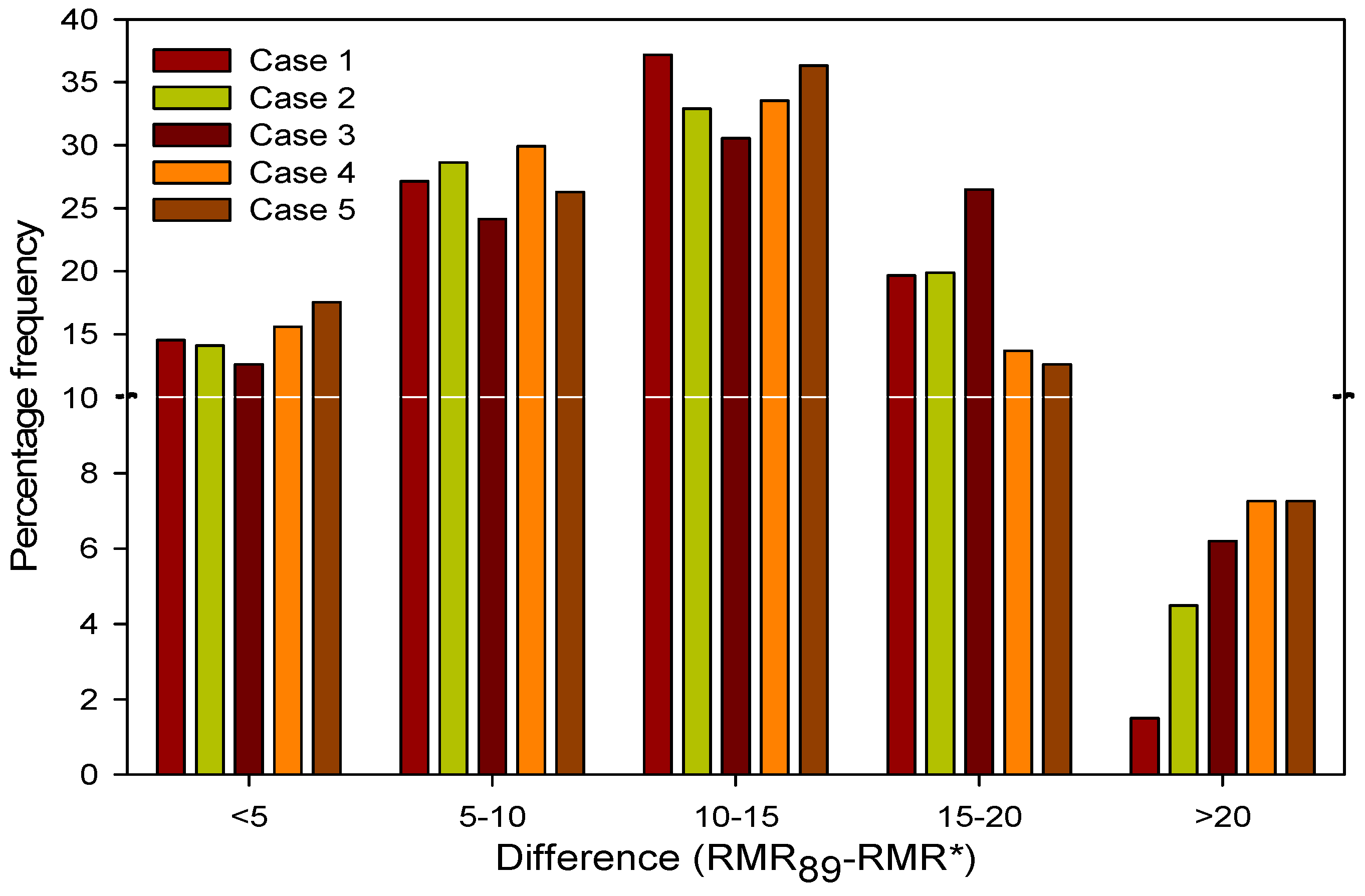
The rock-mass quality was calculated using Equation (1) for the 542 tunnel sections of the four tunnel projects following the two approaches of calculating rock-mass quality through characterization (RMR₈₉) and back-calculation (RMR*). All the five cases of Table 6 were considered in the RMR* calculation. Of the 542 tunnel sections, 468 sections show that RMR₈₉ > RMR* for all the five cases of weightage. The cases that show the difference (RMR₈₉-RMR*) as a positive value are plotted in Figure 2.

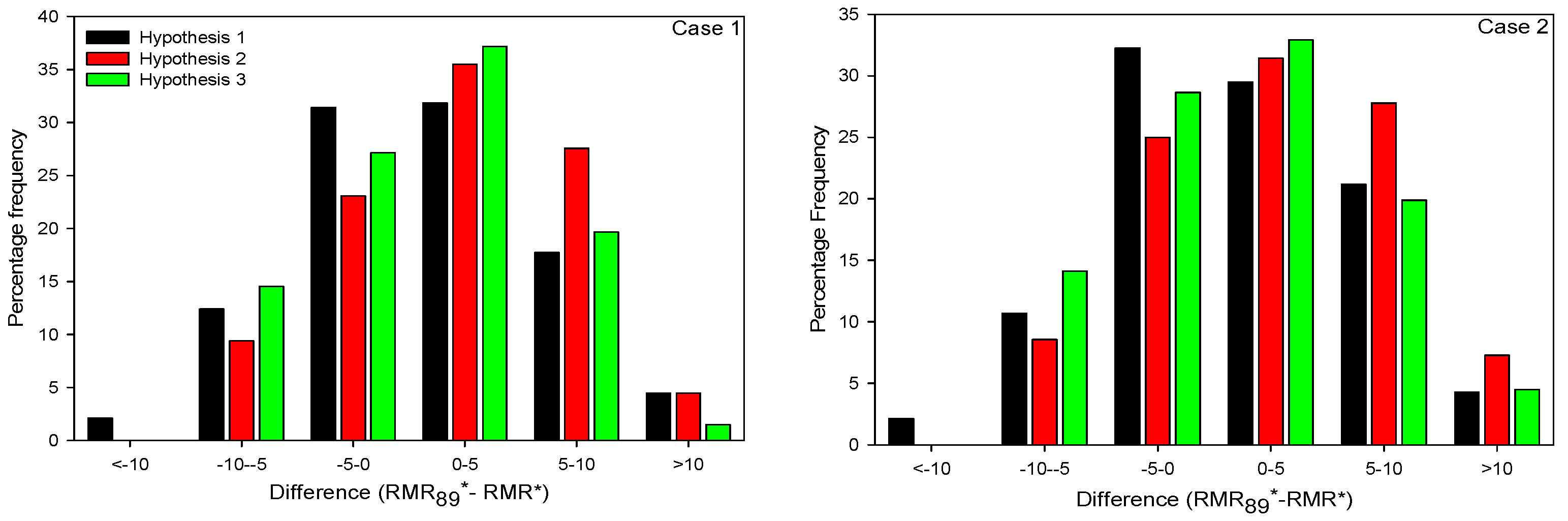
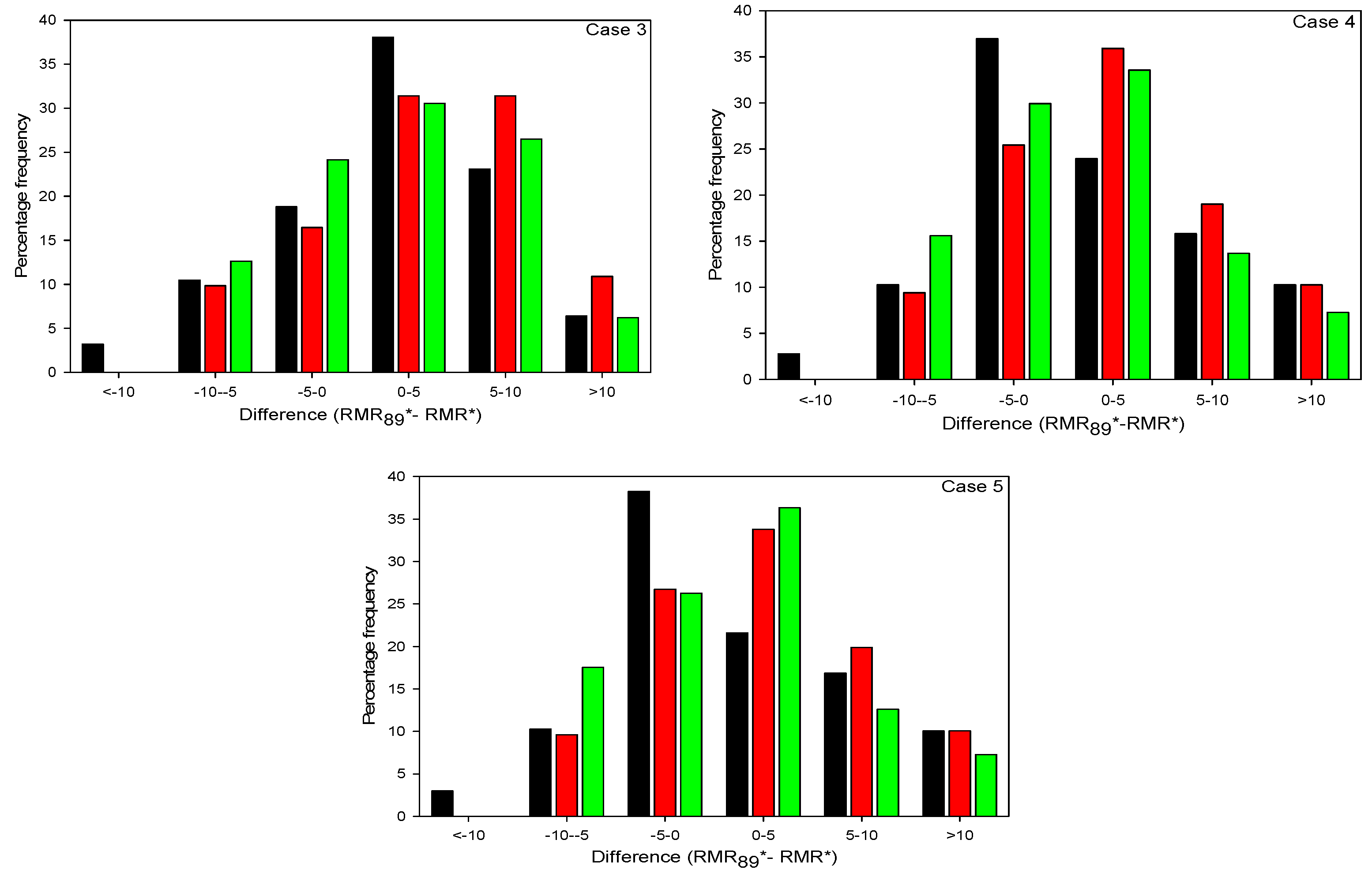
To evaluate the effect of the weightage for all the five cases in the stress adjustment factor for RMR₈₉, three hypotheses were adopted for the F_stress−89. These hypothesis were also used for the extension of the RMR₈₉ application for the rock-mass quality determination in highly stressed jointed rock-mass environments [16]. The details of the hypothesis tested for the rating selection based on intact rock strength to major principal stress (σ₁) ratio (σ_c/σ₁) are shown in Table 3.

Using Equation (14), after applying the stress adjustment factor F_stress−89, based on the selection criterion expressed in Table 3 for all the 468 tunnel sections, RMR₈₉ was adjusted for the stress parameter (RMR₈₉*). The RMR* was calculated using five different weightages of Table 6. For each case, the RMR₈₉* and RMR* are compared in terms of their difference (RMR₈₉*-RMR*) for all the five cases of weightage and for three hypotheses and the obtained results are expressed in Figure 3.

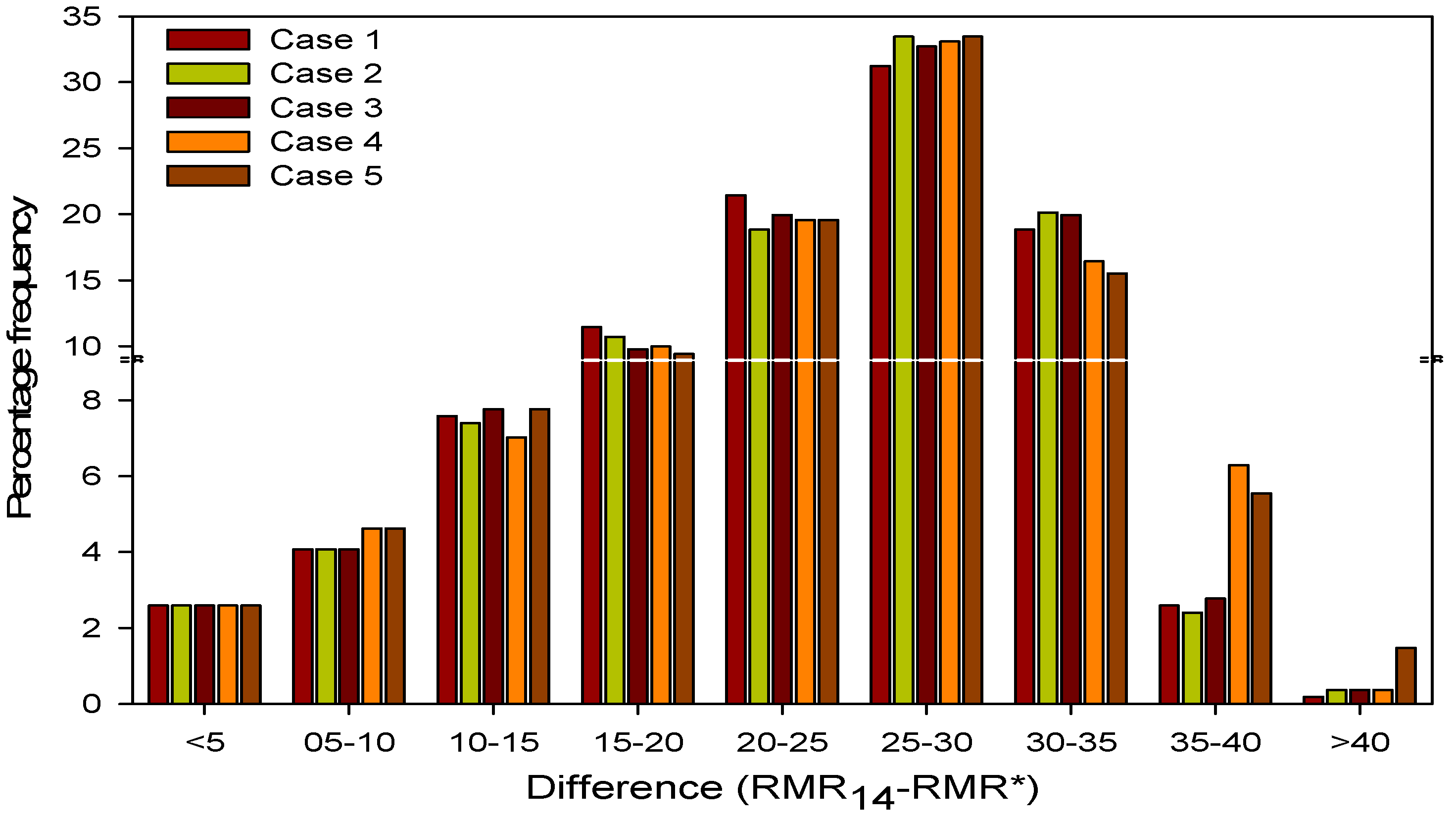
In case of RMR₁₄, the rock-mass quality was calculated using Equation (5) for the 542 tunnel sections of the four tunnel projects through characterization and was compared with the back-calculated RMR while considering all the five cases of Table 6. The comparison between the calculated RMR (RMR₁₄) and back-calculated RMR (RMR*) for all the sections reveal that RMR₁₄ > RMR* for all the five cases, and the details in terms of their difference (RMR₁₄-RMR*) are shown in Figure 4.

To evaluate the effect of the weightage for all the five cases in the stress adjustment factor for RMR₁₄, the three hypotheses were considered for the stress adjustment factor (F_stress−14). The details of the hypothesis tested for the rating selection based on (σ_c/σ₁) for RMR₁₄ are summarized in

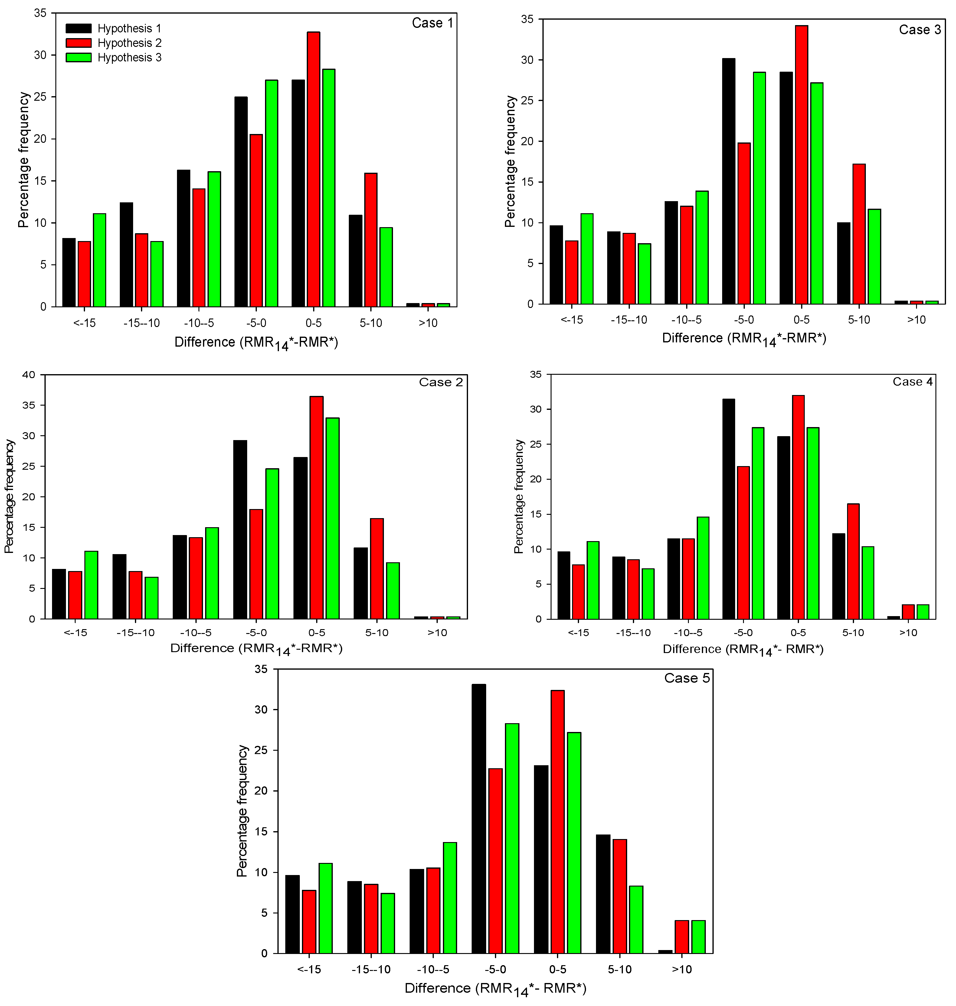
Table 8. Hypothesis used for the F_stress−14 in tunnel support design.

Hypothesis		Values of σc/σ1
		4–5	3–4	2–3
1	Fstress-14	−22.326	−27.169	−32.012
2		−22.326	−27.169	−27.169
3		−27.169	−27.169	−27.169

.

Using Equation (16), after applying the stress adjustment factor based on the selection criterion expressed in Table 7 for all the tunnel sections, RMR₁₄ was adjusted for a stress parameter as RMR₁₄* using Equation (16). The stress-adjusted RMR₁₄ (RMR₁₄*) and RMR* are compared in terms of their difference (RMR₁₄*-RMR*) for all the five cases of weightage and for the three hypotheses, and the obtained results are expressed in Figure 5.

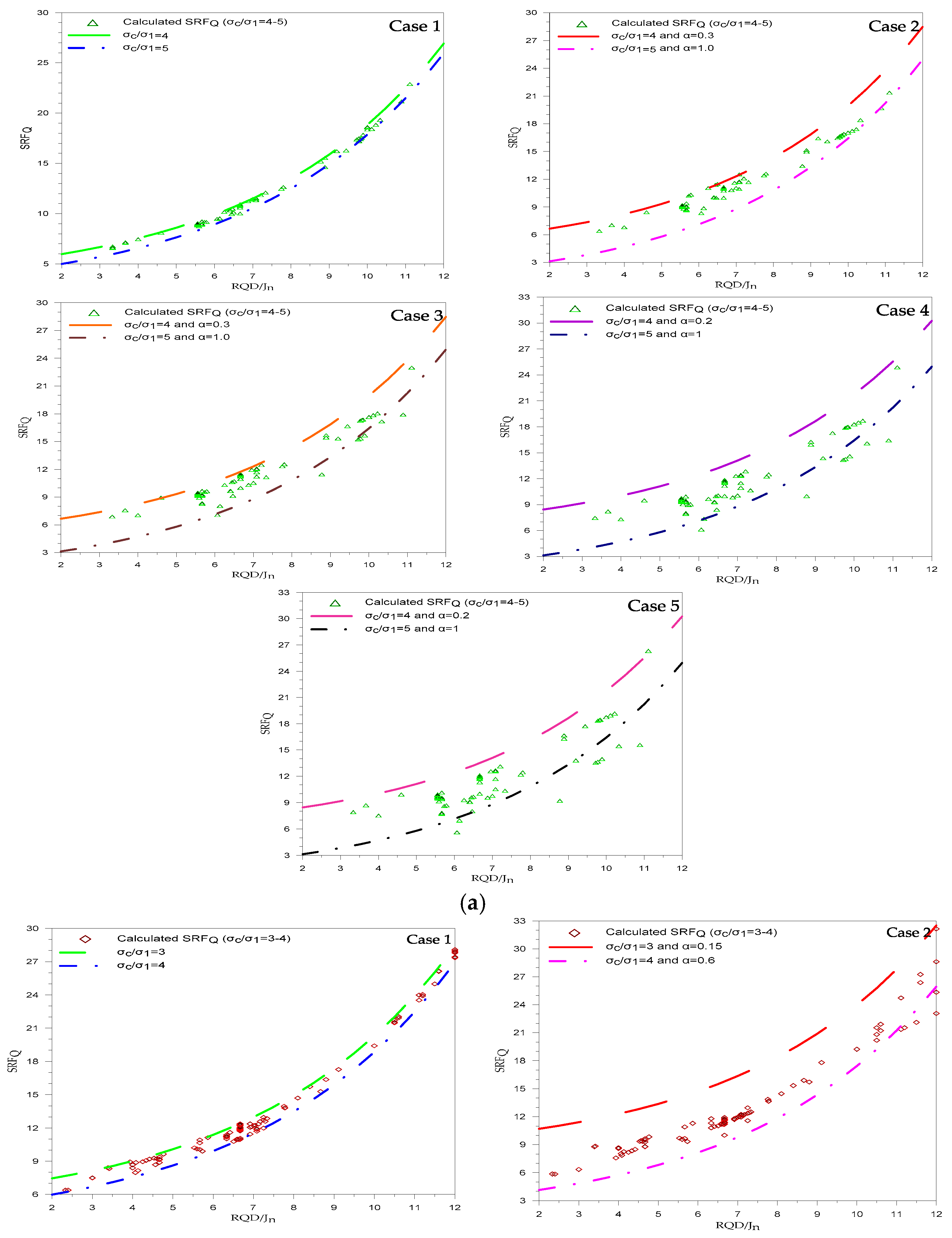
The data of the 542 tunnel sections (as summarized in Table 5) were used in Equation (17). For Equation (17), the back-calculation rock-mass quality (Q*) was determined using the five different weightages of Q₁* and Q₂* as per the details in Table 6. On separating the number of cases based on σ_c/σ₁ from the 542 sections, 156 tunnel sections were found to have this ratio in the range of 4 to 5. In the range of 3 to 4, 232 cases exist, and the remaining 154 sections have a strength–stress ratio in the range of 2 to 3. Cases 1 and 3 of Table 6 are already respectively used for the extension of the application of the Q system of Barton and the rock-mass index (RMi) system of Palmstorm for a highly stress-jointed rock-mass environment [16,17]. The back-calculated rock-mass quality in Figure 1 for all the five cases of weightage was taken as the Q value in Equation (17) for the calculation of the SRF (SRF_Q). This SRF_Q was plotted against the relative block size (RQD/J_n) for different ranges of strength–stress ratio for all the five cases of Q* based on their weightage (Table 6). The results are shown in Figure 6. The best fit equation for Case 1 is Equation (19), and for the remaining four cases is Equation (20). Equations (19) and (20) are already suggested for Case 1 and 3, respectively [16,17]. For Case 2, the best fit Equation (20) has the same values for the constant α. However, in Cases 4 and 5, the constant α values are different, as shown in Figure 6.

$$SR{F}_Q=2.054\exp \left(0.205\frac{RQD}{J_n}\right)+14.865\exp \left(-0.41\frac{{\sigma }_c}{{\sigma }_1}\right)$$

(19)

$$SR{F}_Q=2.0\times \exp \left(0.21\times \frac{RQD}{J_n}\right)+12.0\times \exp \left(-\alpha \times \frac{{\sigma }_c}{{\sigma }_1}\right)$$

(20)

4. Discussion

The already supported tunnel sections data is used in this article. The same data is used for the extension of the RMR [18,19], tunneling quality index [12,26], and RMR index [29] in highly stressed jointed rock-mass environments [16,17]. For the extension process, the back-calculation approach is used for the calculation of the rock-mass quality. In the back-calculation approach, the rock bolt spacing and shotcrete thickness are used along with the tunnel span for determining the rock-mass quality. As can be observed from Figure 1, the final rock-mass quality depends on the rock-mass quality obtained from the rock bolt spacing and shotcrete thickness in combination with the tunnel size. Although the average weightage is used for the calculation of the final rock-mass quality, owing to the unavailability of any criterion, the different weightage effect was not studied. Therefore, five different weightages were selected for the final rock-mass quality determination as shown in Table 6, and the obtained results are presented. For illustration, an example is used, the results of which are summarized in Table 7.

Approximately 86% of the data shows that the back-calculated RMR (RMR*) is lower than the calculate RMR (RMR₈₉) obtained using Equation (1), which indicates that the RMR₈₉ suggested supports are lighter than the actual support. This difference is shown in Figure 2 in terms of the difference between RMR₈₉ and RMR* and reveals that for all cases of weightage, this difference is highest in the rage of 10 to 15 points of RMR. In each range of difference (<5, 5–10, 10–15, 15–20, and >20) the average vales for the five cases are 14.87, 27.22, 34.10, 18.46, and 5.34 with a standard deviation of 1.83, 2.21, 2.68, 5.59, and 2.43, respectively. This shows that for all the five ranges of differences, the deviation from the average of the five cases is very low except in the case of the range of 15–20, wherein the deviation is 5.59. This high deviation is due to the higher frequency of Case 3 with respect to other cases in the range 15–20. The percentage frequency of the difference between RMR₈₉ and RMR* (RMR₈₉-RMR*) in the range of 5 to 20 decreases with the case number, and these values are 84, 82, 81, 77, and 75 for Case 1—5, respectively. As the weightage of the rock-bolts-based back-calculated RMR (RMR₁*) decreased along with the increase in the shotcrete-based RMR (RMR₂*), the percentage frequency decreased. This decrease is due to the higher value of RMR₁* than RMR₂* in the maximum tunnel sections. After the application of the stress adjustment factor based on the strength–stress ratio as per the guidelines of Table 3, the percentage frequency of the difference between the stress-adjusted RMR (RMR₈₉*) and RMR* is the greatest in the range of −5 to 5 for all the five cases of the weightage except Case 3 and Hypothesis 2, as shown in Figure 3. For this case, the percentage frequency is 48 for (RMR₈₉*-RMR*) in the range of −5 to 5. Hypothesis 1 of Table 3 was selected as the stress adjustment factor based on strength–stress ratio obtained for RMR₈₉ [16]. The leading case in terms of percentage frequency, where (RMR₈₉*-RMR*) is in the range of −5 to 5 for Hypothesis 1, is Case 1 followed by Cases 2–5. Their values are 63, 62, 61, 60, and 57, respectively.

RMR₁₄ is the latest version of the RMR system, and therefore, the result of this version and RMR* are compared for each section and expressed in Figure 4 in terms of their difference. In each range of difference, in Figure 4, the percentage frequency of each case is very close with a very low value of standard deviation. The maximum standard deviation is obtained for the difference range 30–35 with a value of 2.09 from the average value of 18.19. As the RMR₁₄ values are higher than RMR₈₉, as shown in Table 2 and Equation (15), the difference (RMR₁₄-RMR*) is greater than that between RMR₈₉ and RMR* (RMR₈₉-RMR*), as shown in Figure 4. Figure 4 reveals that for all the cases of weightage, this difference (RMR₁₄-RMR*) is greatest in the range of 20 to 35 points of RMR. In terms of the percentage frequency, their values are 72, 72, 73, 69, and 69 for Cases 1–5, respectively. Based on the correlation Equation (15), RMR₁₄ decreases significantly with the stress adjustment factor for all the hypotheses of Table 8. After the application of the stress adjustment factor based on the strength–stress ratio as per the guidelines of Table 8, the percentage frequency of the difference between the stress-adjusted RMR₁₄ (RMR₁₄*) and RMR* is greatest in the range of −5 to 5 following all the five cases of weightage. Hypothesis 1 of Table 7 for Case 3 is used for the stress adjustment factor for RMR₁₄ [16]. The leading case in terms of the percentage frequency for the difference between RMR₁₄* and RMR₁₄ (RMR₁₄*-RMR*) in range of −5 to 5 is Case 3 with a value of 58.6 followed by Cases 1, 2, 4, and 5 with values of 57.5, 56.2, 55.6, and 51.9, respectively. Comparing this difference (RMR₁₄*-RMR*) with the difference in RMR₈₉ (RMR₈₉*-RMR*), the percentage frequency in the range of −5 to 5 is lower. These lower values are due to the selection of the stress adjustment factor based on the correlation equation, wherein the data are somewhat scattered from the trend line (R² < 1.0). Secondly, on comparing Figure 3 and Figure 5, the difference in the RMR₁₄ case is more on the negative side as compared to the difference in RMR₈₉, wherein the difference is more on the positive side.

According to the Grimstad and Barton [30], massive rocks have a greater probability of the occurrence of rock burst in a high-stress environment and suggest a higher rating for the SRF in their revised criterion based on relative block size. Their criterion is used for the rock burst occurrence evaluation [31]. In case of a jointed rock mass under high stresses, the SRF is the function of the strength–stress ratio and relative block size along with the intact rock strength [16,17]. The effect of the weightage during the determination of the rock-mass quality through back-calculation as per the details of Table 6 along with procedure of Figure 1 and their corresponding effect on the SRF value using Equation (17) are shown in Figure 6. The line trends in all five cases show that the rate of increase in SRF with the relative block size increases. In Case 1, the variation of SRF is 20.95 for RQD/Jn from 2 to 12 for all the three ranges of the strength–stress ratio. 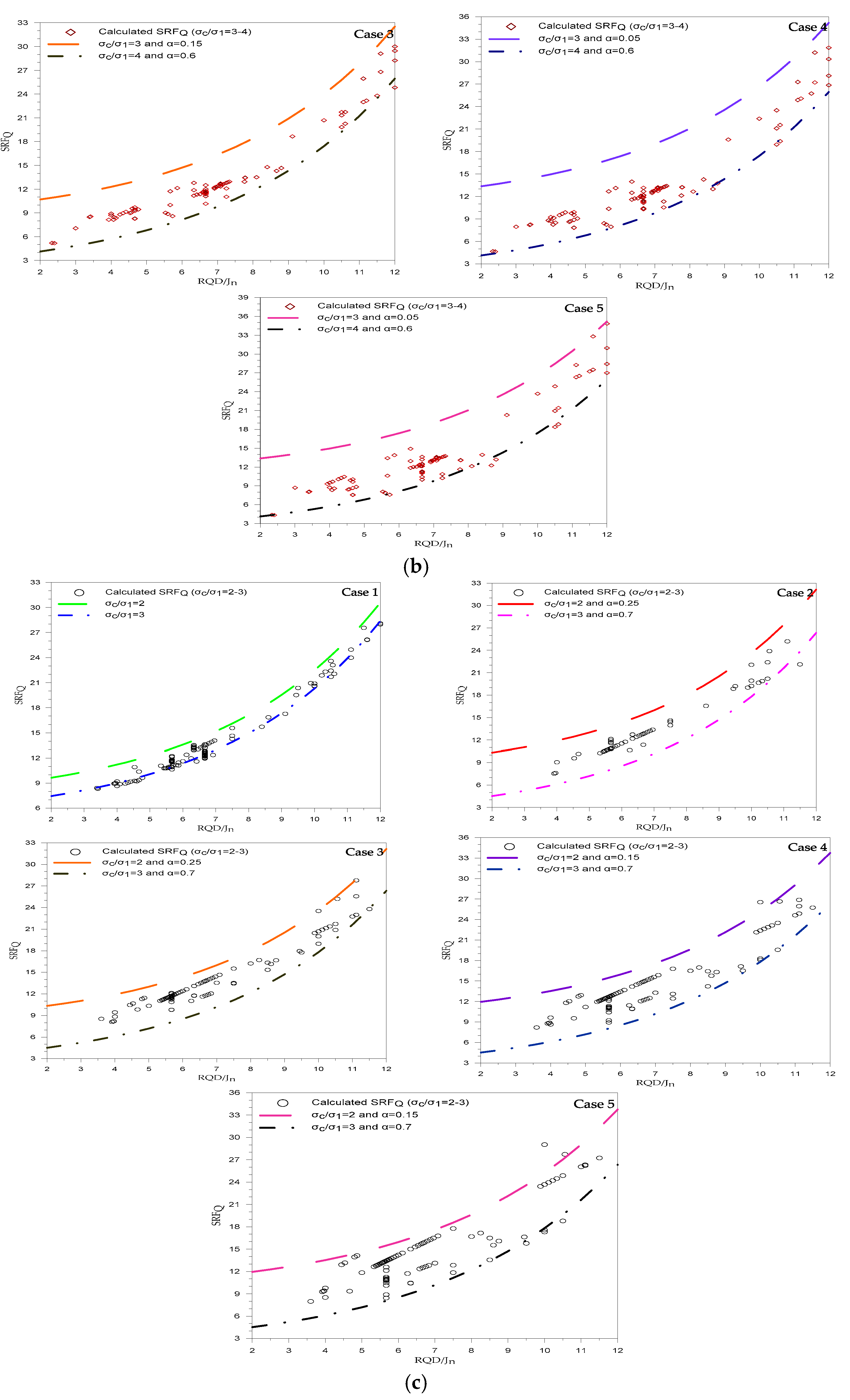The Case 1, Figure 6a–c shows that as the strength–stress ratio range changes from 2–3 to 3–4 and then 4–5, the difference between the trend lines for any given value of relative size decreases. These values are 2.2, 1.46, and 0.97, respectively. In all the remaining cases, the differences are controlled by the difference in values of the constant α in each case and the strength–stress ratio range. In each range of the strength–stress ratio, Cases 2 and 3 have the same difference in α. Similarly, Cases 4 and 5 have the same difference in α. For Cases 2 and 3, the differences in α are 0.7, 0.45, and 0.45 for the strength–stress ratios 4–5, 3–4, and 2–3, respectively. For Cases 4 and 5, these differences are 0.8, 0.55, and 0.55, respectively. The difference in the trend line in Figure 6a shows that for any values of relative block sizes, the difference between the SRF for strength–stress ratios 3 and 2 are 5.81 for Cases 2 and 3 and 7.42 for Cases 4 and 5. In Figure 6b, where the trend lines are shown for strength–stress ratios of 3 and 4, the difference between the SRF increases for the given value of the relative block size. These values are 6.56 for Cases 2 and 3 and 9.24 for Cases 4 and 5. In Figure 6c, where the trend lines are shown for the strength–stress ratios of 4 and 5, the difference between the SRF decreases for the given value of the relative block size. The difference between the SRF for any given value of RQD/Jn are 3.53 for Cases 2 and 3 and 5.3 for Cases 4 and 5.

5. Conclusions

The following conclusions are obtained from this study:

• During the back-calculation of the rock-mass quality (RMR* and Q*), the difference between the rock-mass quality obtained from the rock bolt spacing (RMR₁* and Q₁*) and fiber-reinforced shotcrete thickness along with the tunnel span (RMR₂* and Q₂*) are responsible for the weightage effect. The weightage effect is more pronounced when the difference between the back-calculated rock-mass quality from the rock bolts spacing and shotcrete thickness is high and vice versa.
• So far, the back-calculation approach is used for the extension of empirical classification systems to highly stress-jointed rock-mass environment and due to low difference between the back-calculated rock-mass quality through different support media, the weightage effect is small. However, using this approach for the extension of RMR and Q systems to other ground behaviors during tunnel construction and stability, selection of appropriate weightage is the key to evaluate the contribution of rock bolt and shotcrete.
• By increasing the weightage of the shotcrete along with the tunnel-span-based back-calculated rock-mass quality (RMR₂* and Q₂*), the RMR* and Q* values are high if RMR₂* > RMR₁* and Q₂* > Q₁* and vice versa. Owing to the structure of RMR and Q value calculation in the two systems, the consequence of low weightage effect is higher in the Q system as compared to the RMR system.
• In the case of the Q system, on using the five weightage cases, the plot trend of the stress reduction factor SRF_Q versus the relative block size RQD/J_n is the same for all the three ranges of strength–stress ratio (σ_c/σ₁). These trends show that the rate of SRF_Q increases with the relative block size.