Analyzing Spatial Community Pattern of Network Traffic Flow and Its Variations across Time Based on Taxi GPS Trajectories

Abstract

The transport system is a critical component of the urban environment in terms of its connectivity, aggregation, and dynamic functions. The transport system can be considered a complex system due to the massive traffic flows generated by the spatial interactions between land uses. Benefiting from the recent development of location-aware sensing technologies, large volumes of traffic flow data (e.g., taxi trajectory data) have been increasingly collected in spatial databases, which provides new opportunities to interpret transport systems in cities. This paper aims to analyze network traffic flow from the perspective of the properties of spatial connectivity, spatial aggregation, and spatial dynamics. To this end, we propose a three level framework to mine intra-city vehicle trajectory data. More specifically, the first step was to construct the network traffic flow, with nodes and edges representing the partitioned regions and associated traffic flows, respectively. We then detected community structures of network traffic flow based on their structural and traffic volume properties. Finally, we analyzed the variations of those communities across time for the dynamic transport system. Through experiments in Beijing city, we found that the method is effective in interpreting the mechanisms of urban space, and can provide references for administrative divisions.

1. Introduction

Transport systems are of great importance to urban environments for their connectivity, aggregation, and dynamic functions. Land uses are connected by the transport network to improve the accessibility of human activities. Considering the spatial heterogeneity of traffic flows, multiple land uses are also attracted by each other, showing an agglomeration (or aggregation) pattern in the space. In addition, such characteristics of a transport system depend largely on the temporal dimension. Therefore, mining the connectivity, aggregation, and dynamic patterns of transport flows can be helpful for revealing traffic structures and the associated mechanisms of socioeconomic phenomena, e.g., logistics, neighborhood, living habitats, and urban function zones [1,2,3].

In reality, the regionalization of urban areas is often non-adjacent. For example, working areas and residential areas belong to the same group in terms of their functions, while in the physical space, they are often distant from each other. Therefore, only using geometric indicators such as geographic distance to measure the connectivity of land uses of interest is limited, and the potential solution could come from the function space of transport. Instead of the static condition of geometric space, a transport system implies the real interactions between land uses across space and time. For example, in the morning, the interaction between residential areas and working areas is much intense, while at lunch time, the interaction between working areas and catering service areas is more intense. In addition, the interactions of land uses in terms of traffic flows can reveal the traffic conditions on different routes in the urban space. It is believed that different routes serve different roles in the daily transportation. For example, the routes connecting residential areas and working areas are likely to be chosen by commuters in the morning. Besides the main roads, some minor roads, for example detours, could also be favored by residents. However, how to extract the functional associations between land uses remains a challenging task.

Considering the importance of transport systems, many studies have been done to discover the hidden regularities in urban transportation. However, due to limited data sources, it is rather difficult to identify the changes of traffic flows across space and time [1,4]. In addition, China’s transport infrastructures are developing very fast, and the associated transport systems are becoming more complex and dynamic. It is necessary to study the transport system in a more effective and timely way. Benefiting from the recent development of location-aware sensing technologies, there is an unprecedented opportunity for us to obtain big traffic data with agent trajectory information [5,6]. For example, nowadays, most of vehicles are equipped with a global positioning system (GPS), which records the locations and other semantic properties (e.g., speed and direction) of agents. Analyzing these data within the context of a transport system could provide a detailed view of the traffic flow, and then reveal typical spatial interaction patterns in the urban space, e.g., popular routes for driving, associations among land uses, and the spatial structures of urban space.

For example, Ahas et al. [7] used mobile phone positioning data to explore the movement patterns of suburban commuters in Tallinn, Estonia. They found that there is a remarkable temporal rhythm to respondents’ locations. Based on mobile phone data, Sevtsuk et al. [8] also discovered that there is significant temporal regularity in human mobility. Other data sources can be also used to analyze traffic flows, e.g., location data of buses [9], smart card transaction data of subways [10], and taxi trajectory data [11,12].

Compared to other modes of transport, the taxi trajectory has no limitations of a fixed line, and thus is more flexibly able to reflect real traffic flows in an urban environment. There are also many relevant studies analyzing taxi trajectory data under different application contexts. For example, Zheng et al. [13] analyzed taxi trajectory data to construct interaction relationships between local regions, and then applied the result to assist in city planning. Guo et al. [14] and Yuan et al. [15] tried to extract the operation status of a traffic system from taxi trajectory data. To identify the city structure, Zhou et al. [16] proposed a field-based data clustering analysis method to detect the changing patterns of constant hotspot areas and inconstant hotspot areas. Since the pick-up and drop-off points of taxi trajectories often imply facilities of interest, Yue et al. [17] used taxi trajectory data to discover the attractive areas that people often visit, e.g., hot shopping and leisure land uses or living and working areas. Recently, Liu et al. [18] proposed an approach to identify traffic congestion regions and their spatiotemporal distributions from taxi trajectory data. Liu et al. [19] viewed the trips of taxis as a displacement in the random walk model, and found that the distribution of directions of taxi trajectories in Shanghai shows a characteristic northeast east–southwest west dominant direction. In addition, they implemented the Monte Carlo simulation and found that geographical heterogeneity leads to a faster observed decay of trips, and the distance decay effect makes the spatial distribution of trips more concentrated in the urban area. Liu et al. [20] proposed the use of spatially embedded networks and network analysis techniques to model intra-city spatial interactions. Zhou et al. [21] allocated Origin/Destination points to land use parcels for describing regional activities, and then combined a series of relevant indicators to explore the land use patterns of Wuhan city. Pan et al. [22] analyzed the characteristics of the pick-up/drop-off points extracted from taxi GPS trajectories, and, based on these features of pick-up/drop-off points, extracted the regular patterns that correspond to the land-use classes within different regions in Hangzhou city. In addition to these aspects, taxi trajectory data can be also used for human mobility pattern mining [5,23,24] and environmental pollution analysis [25,26].

Most previous studies have focused on the connectivity and aggregation of land uses, and few studies have been conducted to comprehensively understand the spatio-temporal community structures of a transport system. With continuous transportation development, there is an increasingly urgent demand for analysis of the spatial structures of transport flows and their variations across time. In general, a traffic flow can be considered a link that connects two land uses, and thus, with multiple flows of this type, a transport system can be modeled as a weighted graph. In this regard, we can introduce community detection and graph matching methods to explore the complex organization of land uses in a transport flow system [27,28].

In this study, we propose a three-levels framework to mine intra-city vehicle trajectory data and detect the spatio-temporal relationships between land uses in the traffic flow system. Therefore, the main contributions of this study are the following:

• Modeling the connectivity structure of traffic flows. We first constructed a spatially embedded network to model the connectivity of land uses, in which the node represents the partitioned region, the edge represents the linkage between adjacent nodes, and the weight of the edge depends on the volume of traffic flows between the corresponding nodes.
• Extracting the aggregation patterns of land uses (i.e., nodes). Based on the network traffic flow, we then employed a community detection technique (i.e., K-Medoids clustering) to classify all the nodes. Instead of the simple geographic distance, our community detection method takes into account the real traffic volume and graph structure properties. In this way, the land uses that have a strong relationship could be aggregated in the same group.
• Analyzing the dynamic patterns of transportation communities. Since the transport system is a highly dynamic system, we propose a graph matching method to detect the change of network traffic flows across time. In this way, we can not only identify the structure of traffic flows across space, but also its variation across time.

The rest of this paper is organized as follows. Section 2 introduces the related definitions, and how to construct the network traffic flows and to generate the communities. To explore the variation of communities across time, this section then introduces an indicator to measure the similarity of two communities. Section 3 describes our extensive experiments based on the taxi trajectory data in Beijing, showing the potential of the proposed approach for transport system analysis and urban applications. Finally, Section 4 concludes the paper.

2. Community Detection across Space and Its Variation across Time

Our method improves the traditional K-Medoids method based on traffic flow volume and network structure properties. Firstly, we partition the study region into equally sized square cells, and then model each cell as a node and the connectivity between each pair of cells as a link. Based on the network traffic flow, we propose that the similarity of nodes can be calculated based on the attraction degree and structure similarity. In this way, community clustering can be implemented. Finally, we use the graph matching technique to calculate the similarity between the community structures within different time periods. Therefore, our method can be considered a spatio-temporal analysis tool.

2.1. Network Construction and Its Variation with Different Cell Sizes

2.1.1. Network Construction

Due to signal loss or degradation, taxi trajectories are usually recorded with spatial uncertainty. Even if a set of trajectory flows comes from (or drives to) the same regions, the recorded trajectory points are unlikely to share the same coordinates. Therefore, in order to extract the collective regularities from these massive trajectory points, our method proposes that the study region be partitioned into equally sized square cells, each of which represents a place in the urban space. In this way, each trajectory point could be assigned to its nearest cell, and a traffic flow consisting of multiple trajectory points could be represented as a set of partitioned cells. More specifically, by specifying the cell size k, the whole region would be transformed into a grid of size k × k. There are also other ways to partition the region, e.g., traffic analysis zones (TAZs). However, TAZs are constrained to a fixed scale, and our method can be used for multi-scale spatial analysis with different cell sizes (please see Section 3). In general, for fine scale applications, a small cell can be used, while for coarse scale applications, a large cell would be used. With the tessellation of space, we can then define the nodes and edges of network traffic flow as follows.

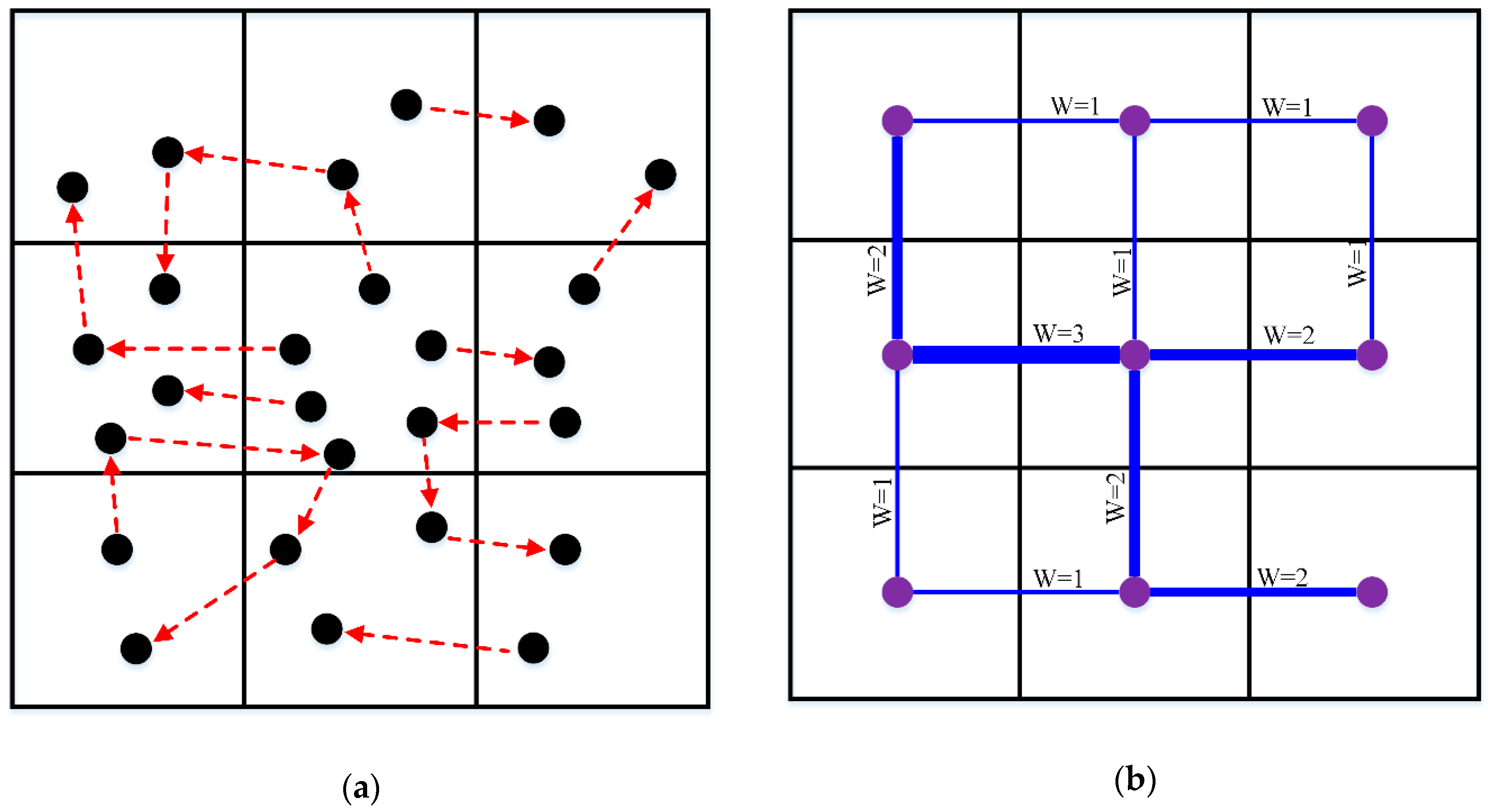
Definition 1.

(Node): Assuming the range of Euclidean coordinates of a cell C is {[$x_{min}$, $x_{max}$], [$y_{min}$, $y_{max}$]}, this cell can be modeled as a node only when there is at least one trajectory point (with coordinate (x, y)) falling into the cell. Specifically, this constraint can be formalized as follows.

$${\begin{array}{c}{x}_{min}<x\le x_{max}\\ y_{min}<y\le y_{max}\end{array}}_{}$$

(1)

Definition 2.

(Edge): Assuming there are n trajectory flows between nodes C₁ and C₂, the connectivity between C₁ and C₂ can be modeled as an edge with weight n. As presented in Figure 1, the weighted edge is used here to represent the flow transitions between cells (i.e., sub-regions).

The movement of vehicles implies the complex interaction between land uses, and connects distant regions into an integrated system. Since the basic characteristic of this system is connectivity, we propose the construction of a spatially embedded network consisting of nodes (Definition 1) and edges (Definition 2) to represent traffic flow. Based on such a network, we can then employ graph analysis techniques (see Section 2.2 and Section 2.3) to discover the hidden regularities in a transport system.

2.1.2. Variation of Network with Different Cell Sizes

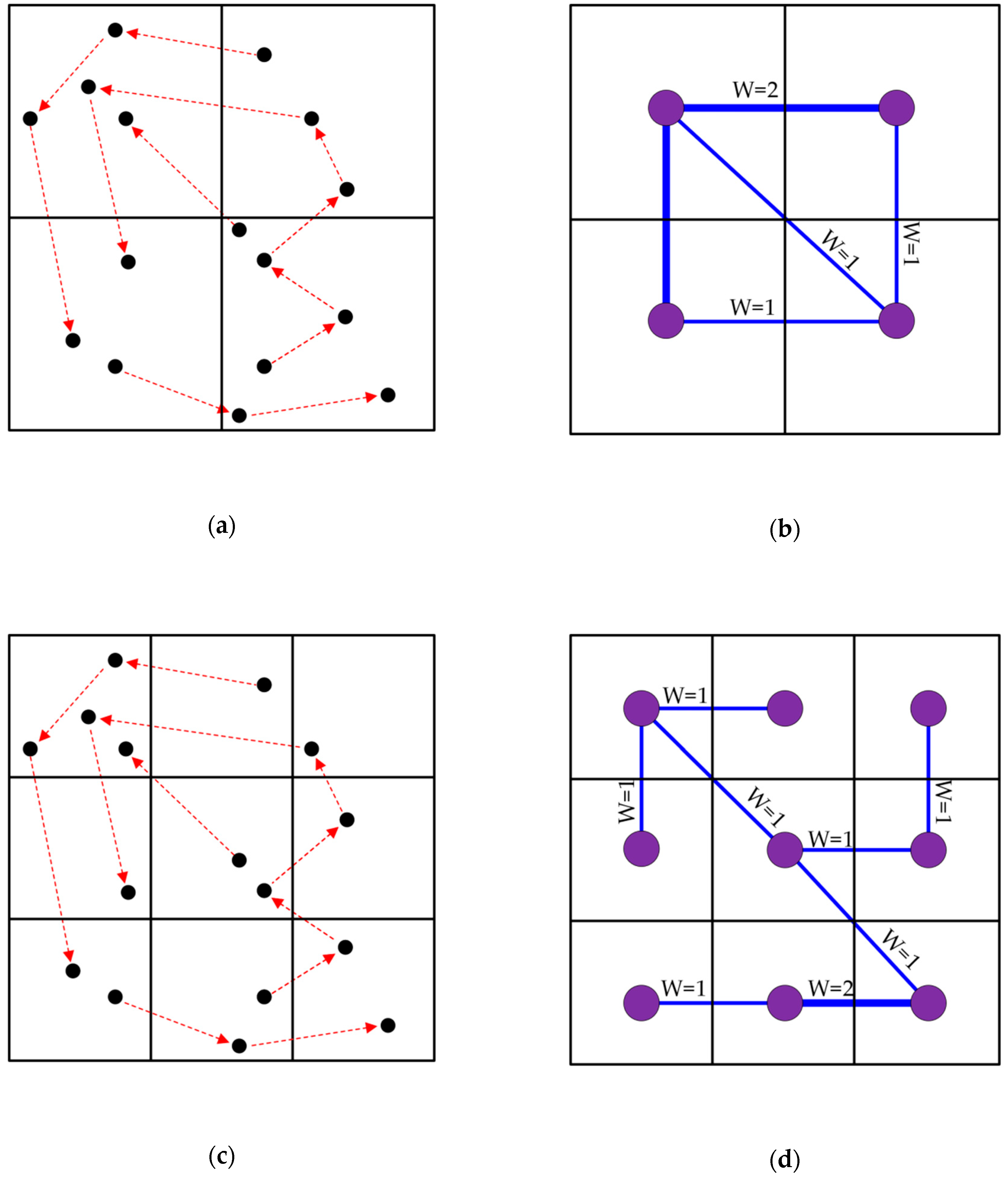
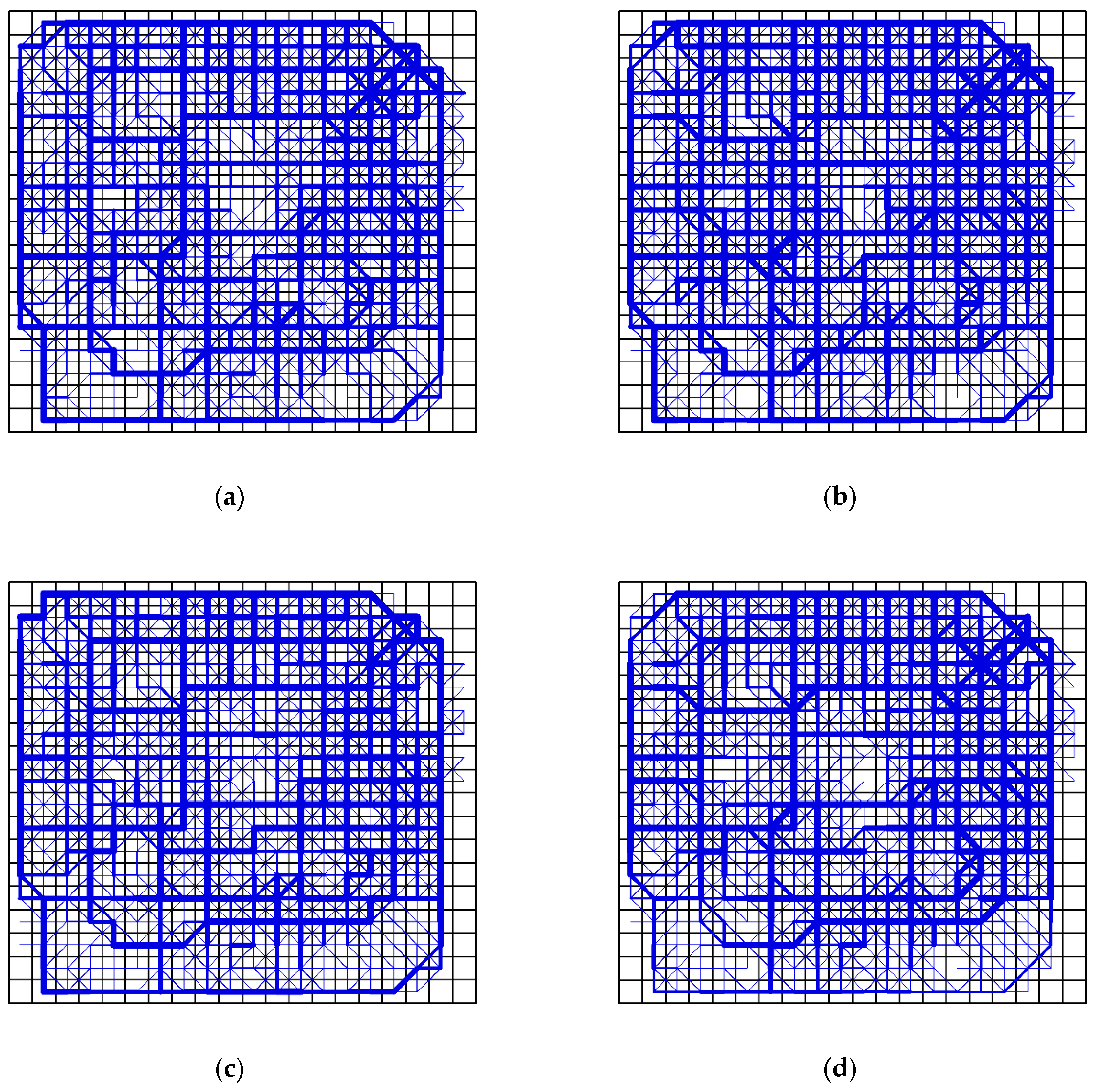
Dividing the whole study area with different cell sizes would make the distribution patterns of trajectory points different, and would also lead to different results in the detection of communities. Figure 2 shows the effect of different cell sizes on the construction of network flows. Although Figure 2a,c have the same trajectory flow, they are divided by different cell sizes. As a result, the constructed networks have different granularities (Figure 2b,c). Therefore, with different cell sizes, we can observe the variation of the network from different scales of space.

2.2. Community Detection across Space

2.2.1. Similarity of Nodes

Besides the connectivity property, a transport system has a spatial heterogeneity in urban space. In other words, some land uses are more attractive to each other in terms of transportation, and in the function space they form aggregation patterns, i.e., community. Such community could imply a popular route at a specific time, or an agglomeration of living areas and work areas. Generally, the more intense the traffic flow interaction between land uses is, the higher probability that the land uses have to be grouped together. Since the transport system is modeled as a spatially embedded network, we can then use the community detection method to extract the clustering patterns of land uses. It should be noted that, compared to the classic graph measures, the concept of community in our context has its own characteristics. Specifically, community detection in a network traffic flow should not only take into account the graph structure factor, but should also consider the traffic flow volumes among different regions. Therefore, we propose that the measures of attraction degree and structure similarity be integrated to group the nodes of network traffic flow.

Before defining the attraction degree, we first introduce the related concept, as follows.

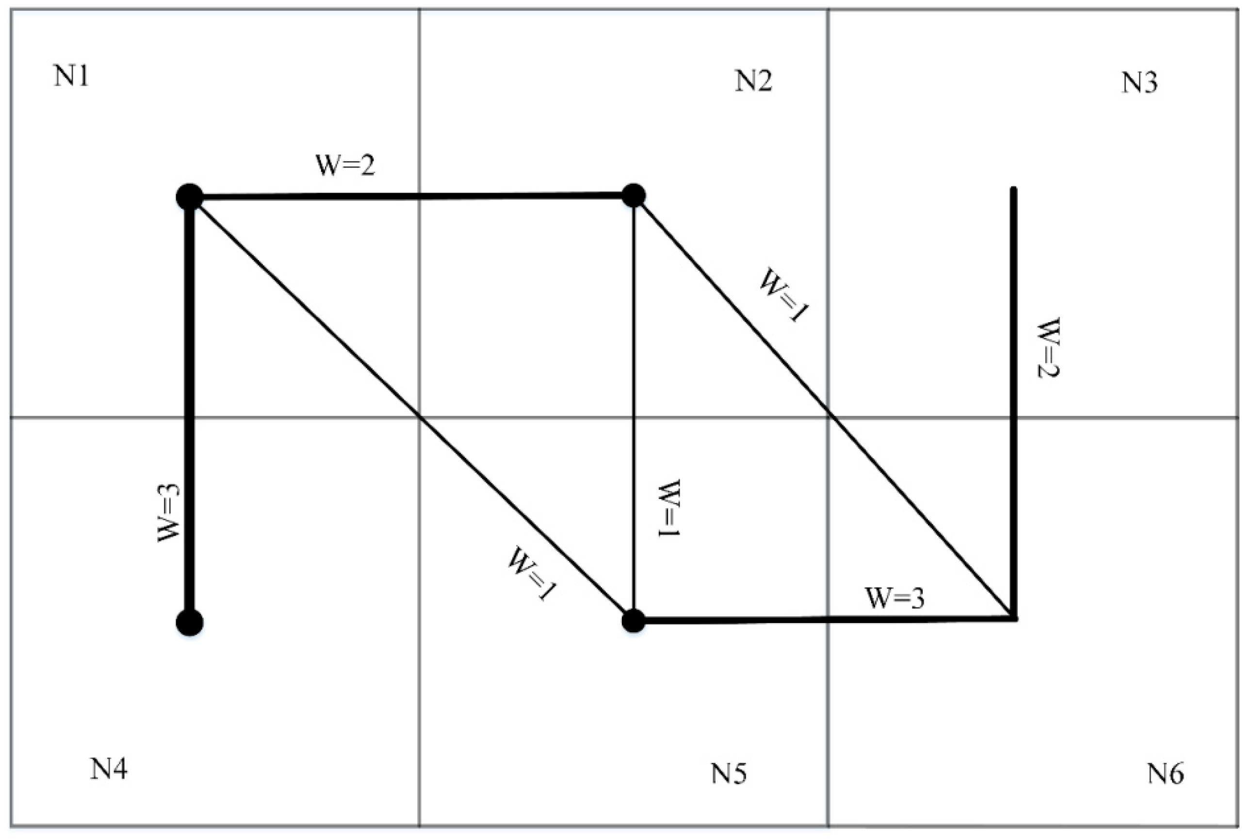
Definition 3.

(Attraction factor): In a network traffic flow, the traffic volume characteristics between a pair of directly connected nodes reveal their closeness relationship, and we term this connection the attracting factor. For the directly connected nodes $N_1$ and $N_2$, their degrees $d_{N_1}$ and $d_{N_2}$ are defined as the number of their connected edges, respectively. Assuming the edge between $N_1$ and $N_2$ is $E_{\left(N_1,N_2\right)}$ with associated weight $W_{\left(N_1,N_2\right)}$, the attracting factor $f_{\left(N_1,N_2\right)}$ between $N_1$ and $N_2$ is calculated as follows:

$$f_{\left(N_1,N_2\right)}=\ln (1+\frac{d_{N_1}}{{{\displaystyle \sum }}_{j=1}^{d_{N_1}}{W}_{1j}}\ast W_{\left(N_1,N_2\right)})$$

(2)

In Figure 3, there are six nodes, including $N_1$, $N_2$, $N_3$, $N_4$, $N_5$ and $N_6$, with their associated edges. In this community, $d_{N_1}=3$, $W_{\left(N_1,N_5\right)}$ = 1, ${{\displaystyle \sum }}_{j=1}^{d_{N_1}}{W}_{1j}=3+2+1=6$, $f_{\left(N_1,N_5\right)}=\ln \left(1+\frac{3}{6}\ast 1\right)=0.4055$, $d_{N_5}=3$, $W_{\left(N_5,N_1\right)}=1$, ${{\displaystyle \sum }}_{j=1}^{d_{N_5}}{W}_{1j}=3+1+1=5$, $f_{\left(N_5,N_1\right)}=\ln \left(1+\frac{3}{5}\ast 1\right)=0.4700$.

Definition 4.

(Attraction degree): Assuming nodes $N_1$ and $N_2$ are directly connected, their attracting degree can be measured as following.

$$Att{r}_{\left(N_1,N_2\right)}=\frac{f_{\left(N_1,N_2\right)}+f_{\left(N_2,N_1\right)}}{2}$$

(3)

In Figure 3, the attraction degree between N₁ and N₅ is $Att{r}_{\left(N_1,N_5\right)}=\frac{f_{\left(N_1,N_5\right)}+f_{\left(N_5,N_1\right)}}{2}=\frac{0.4055+0.4700}{2}=0.43775$.

Definitions 3 and 4 model the force of attraction between any two directly connected nodes (i.e., cells). However, in reality, a node is attracted not only by its directly connected nodes, but also by its indirectly connected nodes. Therefore, we propose the extension of Definition 4 to take into account the attraction degrees from both the directly connected nodes and the indirectly connected nodes. Assuming nodes N_i and N_j are indirectly connected by the path PT (N_i, N_i+1, N_i+2, …, N_j), their attractive degree can be calculated as the product of the attractive degrees of all the pairs of directly connected nodes in PT, i.e., $f_{\left(N_k,N_{k+1}\right)}(i\le k<j)$. The detail is as follows:

$$Att{r}_{\left(N_i,N_j\right)}={{\displaystyle \prod }}_{k=i}^{k=j-1}{f}_{\left(N_k,N_{k+1}\right)}$$

(4)

It should be noted that there might be multiple paths between nodes N_i and N_j, and thus there could be more than one attraction degree value for our analysis. In this regard, we choose the largest-weight path between N_i and N_j to calculate the attraction degree. In general, the nodes directly or indirectly connected by a larger-weight path have a stronger mutual relationship. Compared to the indirectly connected nodes, the directly connected nodes have a higher probability to be attracted by each other.

In Figure 3, there are three paths from N₁ to N₆, including path 1 (PT1: N₁→N₂→N₆), path 2 (PT2: N₁→N₅→N₆), and path 3 (PT3: N₁→N₂→N₅→N₆). The weight of PT1 is W_PT1 = 2 + 1 = 3, the weight of PT2 is W_PT2 = 1 + 3 = 4, and the weight of PT3 is W_PT3 = 2 + 1 + 3 = 6. The largest-weight path, between N₁ and N₆, is PT3. Thus, according to Equation (2) and Equation (3), $Att{r}_{\left(N_1,N_2\right)}$ = 0.8047, $Att{r}_{\left(N_2,N_5\right)}$ = 0.5148, $Att{r}_{\left(N_5,N_6\right)}$ = 0.9730, and thus $Att{r}_{\left(N_1,N_6\right)}=$ 0.8047 × 0.5148 × 0.9730 = 0.4031 (Equation (4)).

Besides the strength of connectivity between nodes, the local structure of a graph is also critical to cluster nodes. More specifically, for any pair of nodes connected by a path, the greater proportion their path weight has in the total weight of their neighbors, the more similar the two nodes are. In a local structure, the nodes with a relatively stronger linkage tend to be grouped together. As a comparison, two nodes with a large connection could also be separated into different groups if one of them were to have another, stronger linkage to other nodes. To this end, we introduce structure similarity into our method, as follows.

Our structure similarity indicator is inspired by the Jaccard similarity coefficient, which has been widely applied to describe the relevance among objects. Assuming X and Y are two sets, the Jaccard similarity coefficient is defined as follows:

$$si{m}_{\left(X,Y\right)}=\frac{\left|X{{\displaystyle \cap }}^{}Y\right|}{\left|X{{\displaystyle \cup }}^{}Y\right|}$$

(5)

In addition, in graph theory, it is believed that the critical structural factors of a graph are the links that have relatively larger weight [29]. In this regard, we define structure similarity based on local edges and associated weights, as presented in Definition 5.

Definition 5.

(Structure similarity): For two directly connected nodes N₁ and N₂, their structure similarity is as follows:

$$si{m}_{\left(N_1,N_2\right)}=\frac{W_{\left(N_1,N_2\right)}}{{{\displaystyle \sum }}_{c=1}^{d_{N_1}}{W}_{\left(N_1,N_{1c}\right)}+{{\displaystyle \sum }}_{c=1}^{d_{N_2}}{W}_{\left(N_2,N_{2c}\right)}-W_{\left(N_1,N_2\right)}}$$

(6)

where $W_{\left(N_1,N_{1c}\right)}$ is the weight of the edge connecting node N₁ and its neighbor N_1c, and $W_{\left(N_2,N_{2c}\right)}$ is the weight of the edge connecting node N₂ and its neighbor N_2c. Equation (6) can be only used to measure the structure similarity of directly connected nodes, and in order to analyze the relationships between indirectly connected nodes, we extend Equation (6), as follows:

$$si{m}_{\left(N_i,N_j\right)}={\displaystyle \prod }_{k=i}^{k=j-1}si{m}_{\left(N_k,N_{k+1}\right)}$$

(7)

where N_k and N_k+1 are two directly connected nodes on the path connecting N_i and N_j.

In addition, we choose the largest-weight path between N_i and N_j to calculate the structure similarity. Generally, the directly connected nodes have a larger structure similarity than the indirectly connected nodes do.

In Figure 3, ${{\displaystyle \sum }}_{j=1}^{d_{N_1}}{W}_{1j}=6$, ${{\displaystyle \sum }}_{j=1}^{d_{N_5}}{W}_{5j}=5$, $W_{\left(N_1,N_5\right)}=1$, $si{m}_{\left(N_1,N_5\right)}=\frac{1}{6+5-1}$ = 0.1. The largest-weight path between N₁ and N₆ is N₁→N₂→N₅→N₆, and, thus, $si{m}_{\left(N_1,N_2\right)}=0.2$, $si{m}_{\left(N_2,N_5\right)}=0.1111,si{m}_{\left(N_5,N_6\right)}=0.2727.$ Therefore, according to Equation (7), $si{m}_{\left(N_1,N_6\right)}=0.2\ast 0.1111\ast 0.2727=0.0061$.

Finally, since both the attraction degree (Equation (4)) and the structure similarity (Equation (7)) have been normalized, we can integrate them into a single measure, as follows:

$$fsi{m}_{\left(N_i,N_j\right)}=si{m}_{\left(N_i,N_j\right)}+Att{r}_{\left(N_i,N_j\right)}$$

(8)

2.2.2. Algorithm

Based on the integrated similarity measure, we then calculated the final distance for each pair of directly or indirectly connected nodes (i.e., cells) in the network traffic flow.

$$fdi{s}_{\left(N_{\mathrm{i}},N_j\right)}=\frac{1}{fsi{m}_{\left(N_i,N_j\right)}}$$

(9)

In the process of detecting community, the dissimilarity index for each pair of nodes is adopted, with which one can measure the extent of proximity between the nodes of a network and signify to what extent two nodes would ‘like’ to be in the same community [30]. This proximity reflects the connectivity property of nodes in a diffusion process. The final minimization problem under this distance can also be solved by a k-means algorithm [31].

For our community detection algorithm, we adopted the K-Medoids algorithm, which belongs to the family of k-means clustering. More specifically, we first calculate the distances between all the pairs of nodes, and then select k nodes (i.e., initial k medoids) which have the largest distance to each other. Secondly, we assign each node (except the nodes that have already been labeled) to its nearest cluster according to the distances measured on the network traffic flow. This process is iteratively conducted until the medoids do not change or the number of iterations is equal to the threshold. In addition, in the end of each iteration, the node that has the minimum sum of distances within the cluster is selected as the medoid. Our community detection algorithm is as follows (Algorithm 1):

Algorithm 1. Community Clustering

Input: A spatially embedded network consisting of nodes and edges with weight, the number of communities k, the maximum number of iterations MaxI. Output: A set of communities: C= {C1, C2, …, Ck} 1. Initialization: $fdi{s}_{\left(N_i,N_j\right)}=0,$ iteration=0, ClusterCentriod [] C=null; 2. Node distance calculating: //calculate the distance between each pair of nodes.   for each pair of nodes Ni and Nj (i ≠ j)     $fsi{m}_{\left(N_i,N_j\right)}=si{m}_{\left(N_i,N_j\right)}+Att{r}_{\left(N_i,N_j\right)}$;     $fdi{s}_{(N_{\mathrm{i}},N_j)}=\frac{1}{fsi{m}_{(N_i,N_j)}}$;   end for   for each pair of nodes Ni and Nj (i = j)     $fdi{s}_{(N_{\mathrm{i}},N_j)}=1$;   end for 3. Community detection based on the K-Medoids framework:   Select k nodes that have the largest distance to each other as initial k medoids, i.e., {C1, C2, …, Ck};   Assign each node to the closest medoid;   While (the medoids do not change or iteration ≤MaxI)     for each node Ni       Assign Ni to the closest medoid Cm with min {$fdi{s}_{\left(N_i,C_m\right)}$};     end for     for each cluster Cj (j≤k)       Update the medoid of each community by detecting the node that has the minimum sum of distances within the cluster;     end for     iteration++;   end while  Return the structure consisting of k communities: C= {C1, C2, …, Ck}.

2.3. Variation of Community across Time

Besides the spatial heterogeneity, a transport system also has the dynamic property, and, in order to analyze such variation of a transport system across time, we propose a graph structure matching measurement (GSMM) between two network traffic flows sharing the node set. Specifically, as presented in previous sections, a network traffic flow in a specific time slice can be divided into several communities. In other words, the variation of a transport system across time can be represented as the change of the corresponding community structures. Hence, the GSMM measures the degree of matching between two community structures, i.e., two node sets.

Definition 6.

(Similarity of two node sets): Let S₁ and S₂ be two node sets, the similarity between S₁ and S₂ is defined as follows:

$$Ssi{m}_{\left(S_1,S_2\right)}=\frac{2\left|S_1{{\displaystyle \cap }}^{}{S}_2\right|}{\left|S_1|+|S_2\right|}$$

(10)

where |S| is the number of the nodes of set S and $\left|S_1{{\displaystyle \cap }}^{}{S}_2\right|$ is the number of the nodes that S₁ and S₂ share. For example, if S₁ = S₂, $Ssi{m}_{\left(S_1,S_2\right)}=1$; if $S_1{{\displaystyle \cap }}^{}{S}_2=\Phi$, $Ssi{m}_{\left(S_1,S_2\right)}=0$.

Equation (10) only measures the similarity between two node sets (i.e., two communities), each of which plays a different role in the corresponding graph structure. Specifically, for a graph, some communities are more important than others, and, in order to measure the global similarity between two graphs (i.e., two sets of communities), we propose calculation of the sum of the weighted similarity between two sets of communities. In this process, we define the weight of a community as its contribution rate in the corresponding graph. In general, the more nodes the community has, the larger contribution rate it has for the whole system. Assuming the graph C consists of the communities {C₁, C₂, …, C_k} and S₁, S₂, …, S_k are the node sets of C₁, C₂, …, C_k, respectively, the contribution rate of C_i (i = 1, 2, …, k) is defined as follows:

$$com{R}_{C_i}=\frac{S_i}{S}$$

(11)

Based on the contribution rate of community, we then calculate the weighted similarity between two network traffic flows as follows.

Definition 7.

(Similarity of spatially embedded networks): Let C_p and C_q be two spatially embedded networks with k-size community structures {$C_1^p$, $C_2^p$, …, $C_k^p$} and {$C_1^q$, $C_2^q$, …, $C_k^q$}, respectively. $com{R}_1^p$, $com{R}_2^p$, …, $com{R}_k^p$ are the contribution rates of the communities $C_1^p$, $C_2^p$, …, $C_k^p$, respectively, and $com{R}_1^q$, $com{R}_2^q$, …, $com{R}_k^q$ are the contribution rates of the communities $C_1^q$, $C_2^q$, …, $C_k^q$, respectively. $S_1^p$, $S_2^p$, …, $S_k^p$ are the node sets of the communities $C_1^p$, $C_2^p$, …, $C_k^p$, respectively, and $S_1^q$, $S_2^q$, …, $S_k^q$ are the node sets of the communities $C_1^q$, $C_2^q$, …, $C_k^q$, respectively. Then, the similarity between the two graphs C_p and C_q is defined as:

$$FsimC=\underset{i_1,i_2\dots i_k}{max}\frac{2\ast Psim{C}_{\left(i_1,i_2\dots i_k\right)}}{{{\displaystyle \sum }}_{j=1}^k\left(com{R}_j^p+com{R}_j^q\right)}$$

(12)

where $Psim{C}_{\left(i_1,i_2,\dots ,i_k\right)}$ is calculated as follows:

$$\begin{gathered} Psim{C}_{\left(i_1,i_2\dots i_k\right)}=\frac{1}{2}\ast \left(com{R}_1^p+com{R}_{i1}^q\right)\ast Ssi{m}_{\left(S_1^p,S_{i1}^q\right)}+\frac{1}{2}\ast \left(com{R}_2^p+com{R}_{i2}^q\right)\ast Ssi{m}_{\left(S_2^p,S_{i2}^q\right)} \\ +\dots +\frac{1}{2}\ast \left(com{R}_k^p+com{R}_{ik}^q\right)\ast Ssi{m}_{\left(S_k^p,S_{ik}^q\right)} \end{gathered}$$

(13)

where $\left(i_1,i_2\dots i_k\right)$ is a full permutation of the set $I=\left\{1,2\dots k\right\}$.

The community structure is a partition of all the land uses (i.e., nodes) of the network traffic flow for a specific time slice. Hence, the variation of networks across time can be analyzed by measuring the similarity between the corresponding community structures. The better the matching between two community structures, the more similar the corresponding traffic conditions in different time slices.

3. Data Sets and Settings

We conducted a series of experiments to explore the transport system of Beijing city using taxi trajectory points. As the capital of China, Beijing is the national political, economic, and administrative center. By the end of 2016, the number of taxis in Beijing had reached 71,600, with a permanent population of 21.729 million. More than 55% of residents take taxis every week [32]. In this paper, we chose the central zone of the city (i.e., the range of latitude 39° 49′ 41″–39° 59′ 17″ N and longitude 116° 15′ 47″–116° 29′ 09″ E) as the study region (Figure 4). The research area is within the third ring area of Beijing. The total number of valid records was more than 20,000,000, which covers a time period of 24 h (from 0 a.m. to 12 p.m.) (Figure 4). Because of signal loss or degradation, geospatial locations of trajectory may have been recorded with spatial and temporal uncertainties. Considering these factors, our data were preprocessed by the provider to indicate whether the record was valid or invalid with respect to the GPS signal. In our research, only the valid records were used. Nevertheless, there were some small deviations in position information relative to the actual position. In this respect, we adopted the technique of region tessellation, which is used to model collective behaviors between regions. The internal variation of the region is not considered. Hence, it can handle small deviations of location information and can be used to reveal the collective travel patterns between regions. In order to have a macroscopic understanding of people′s travel patterns, we extracted the taxi pick-up and drop-off points (Figure 5). It can be observed that the hotspots of pick-up and drop-off points are distributed within the second ring roads of Beijing.

4. Experiment and Result

4.1. Result and Analysis

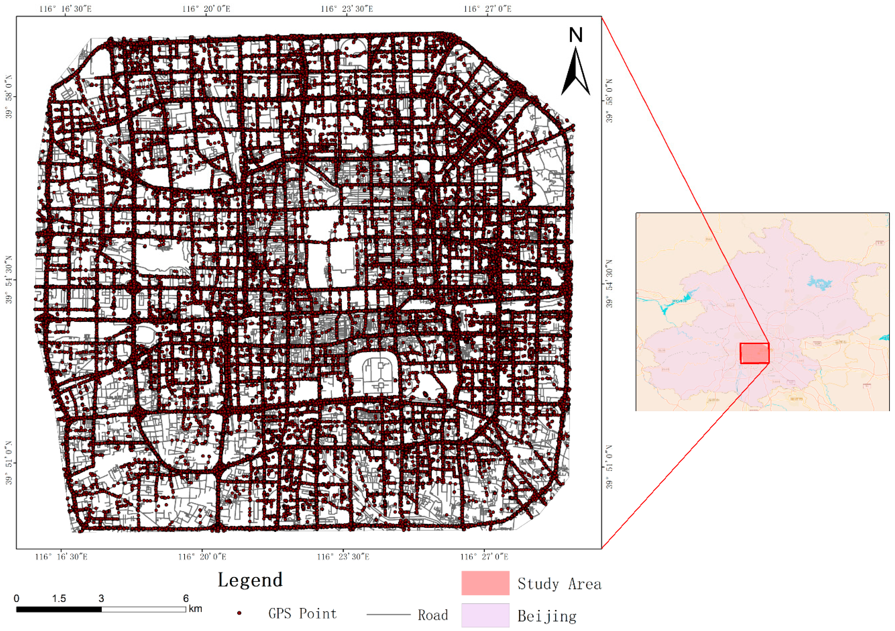
We first partitioned the study area into a set of cells with size 1 km × 1 km. This scale was determined on the basis of relevant studies suggesting that the cell size is fine enough to depict urban structure [33]. We then used these cells to construct spatially embedded networks to analyze the interactions between land uses (i.e., sub-regions). Moreover, we obtained the results in different time periods to discover the dynamic patterns of the transport system.

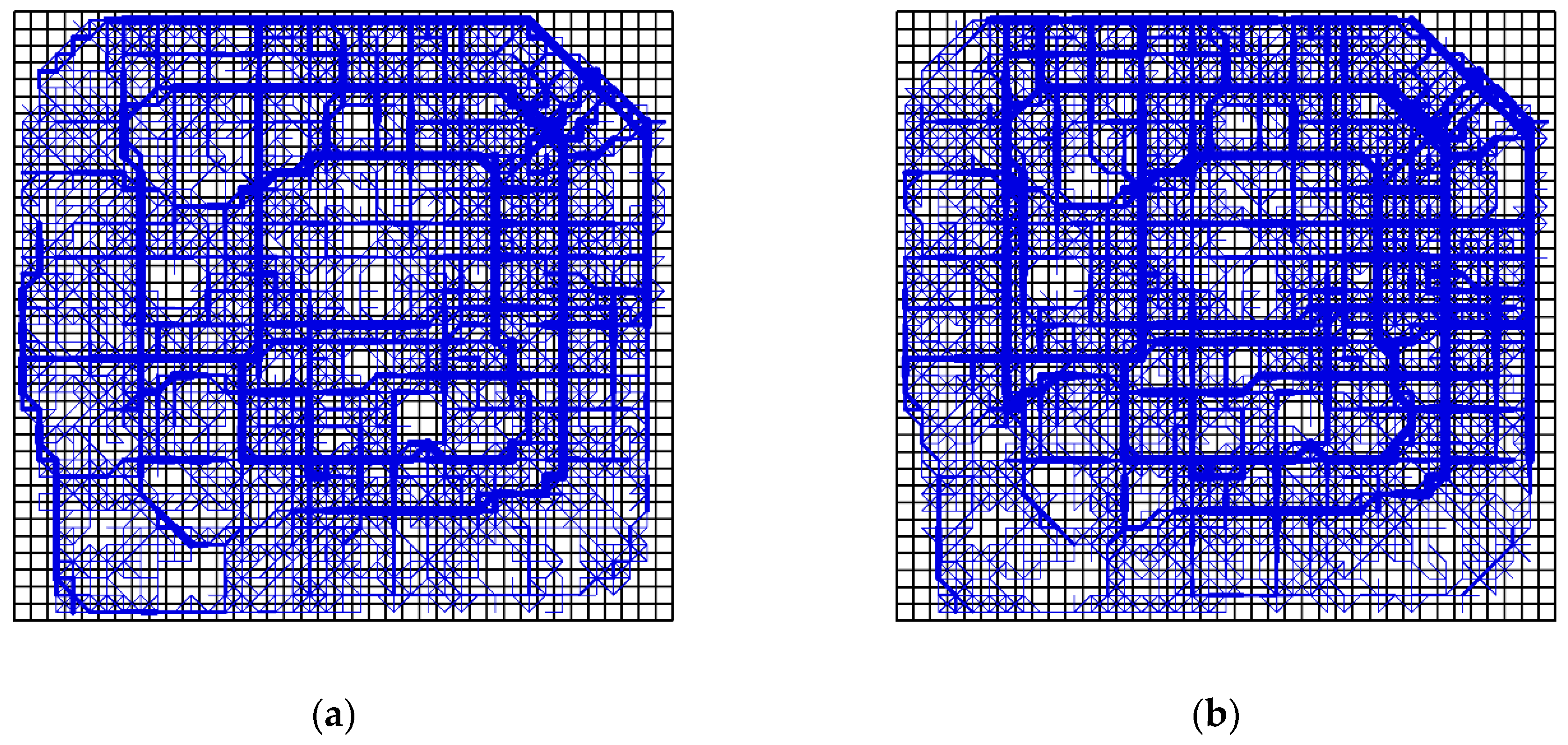
In the spatially embedded network, the nodes represent the regions of the city and the edges represent the traffic linkage between different regions. Furthermore, the intensity of the connections between different regions varies with time. In order to clearly reveal the travel patterns, we constructed networks for typical time periods (Figure 6), i.e., morning rush hour, noon rush hour, evening rush hour, and midnight.

During different time periods of the day, the traffic flows showed different spatial connectivity patterns to meet the varying travel demands of people. In the morning rush hour, the interactions between residential areas, working areas, and schools were more intense than those between the other areas. Later, entering the period of the noon rush hour, the traffic flow volume and the associated connectivity patterns became more significant in the central areas and main roads of the city. Most of the central areas belong to the working zone and commercial zone, and thus the strong connectivity indicates the frequent interactions between working and lunch activities. In addition, although the volume of traffic flows in the evening rush hour was less than that in morning rush hour, their network structures were similar. In Beijing, in order to avoid traffic congestions, many people choose to get off work and go home or go to recreational areas after 19:00. This may be a reason that the traffic volume in evening rush hour was less than that in morning rush hour. Additionally, the routes that people choose to go to work and get off work are similar, and thus the networks in the morning rush hour and evening rush hour had a similar structure. Furthermore, the networks at midnight had a multi-center structure, which depended on the hubs of recreational areas and commercial areas. In general, except the morning rush hour, the other time periods depended more on the eastern areas than the western areas.

Among these hours, the noon rush hour had the largest volume of traffic flows. From the morning rush hour to the noon rush hour, the volume of trajectory flow increased substantially and some new links emerged in local regions. This implies that the interactions between land uses in the noon rush hour are more intense than in the morning rush hour. From the noon rush hour to the evening rush hour, the interactions decreased not only through the main roads but also across the western areas. The obvious feature of interactions at midnight is that there were significant connections to or from recreational land (i.e., the eastern area).

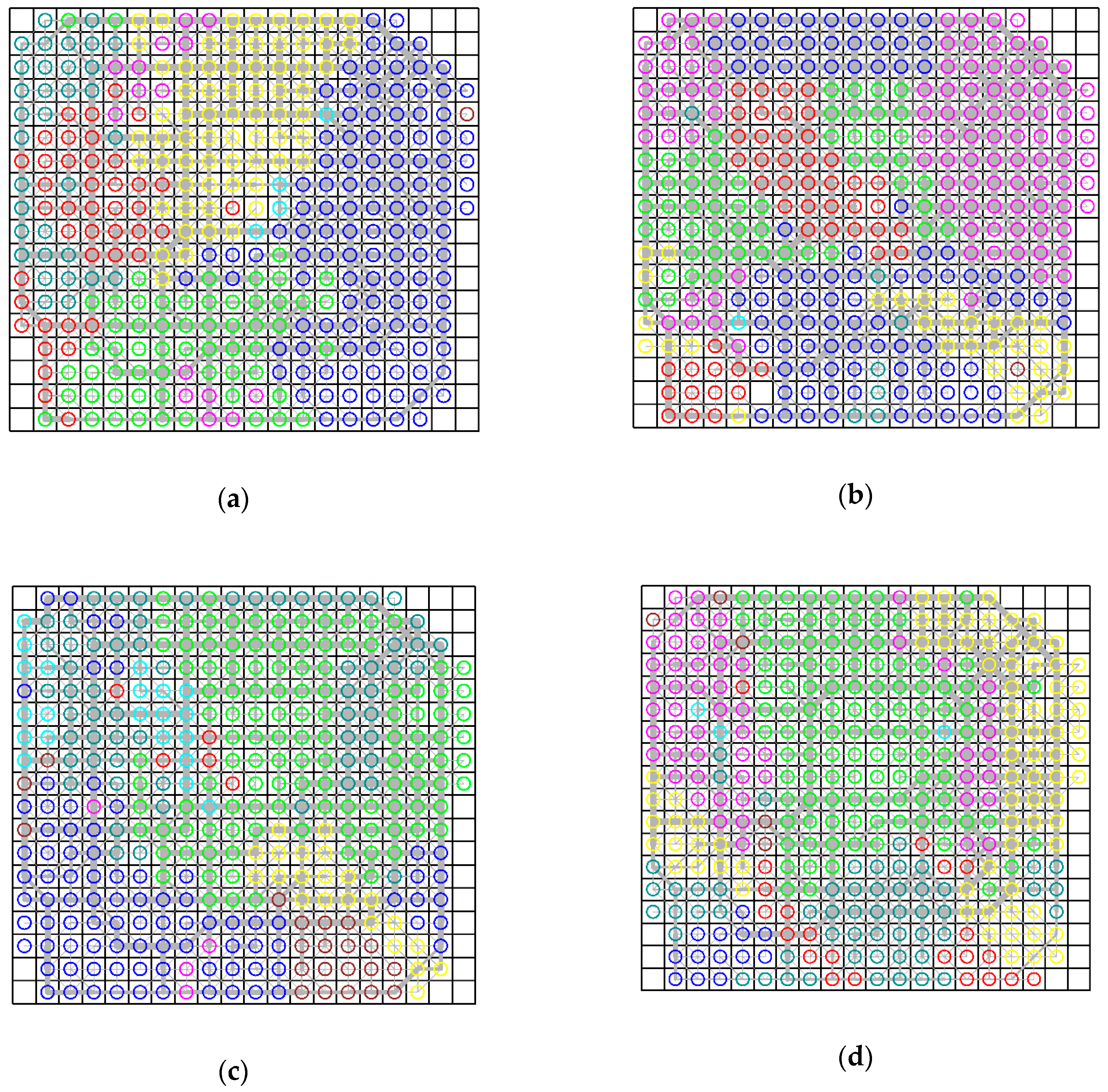
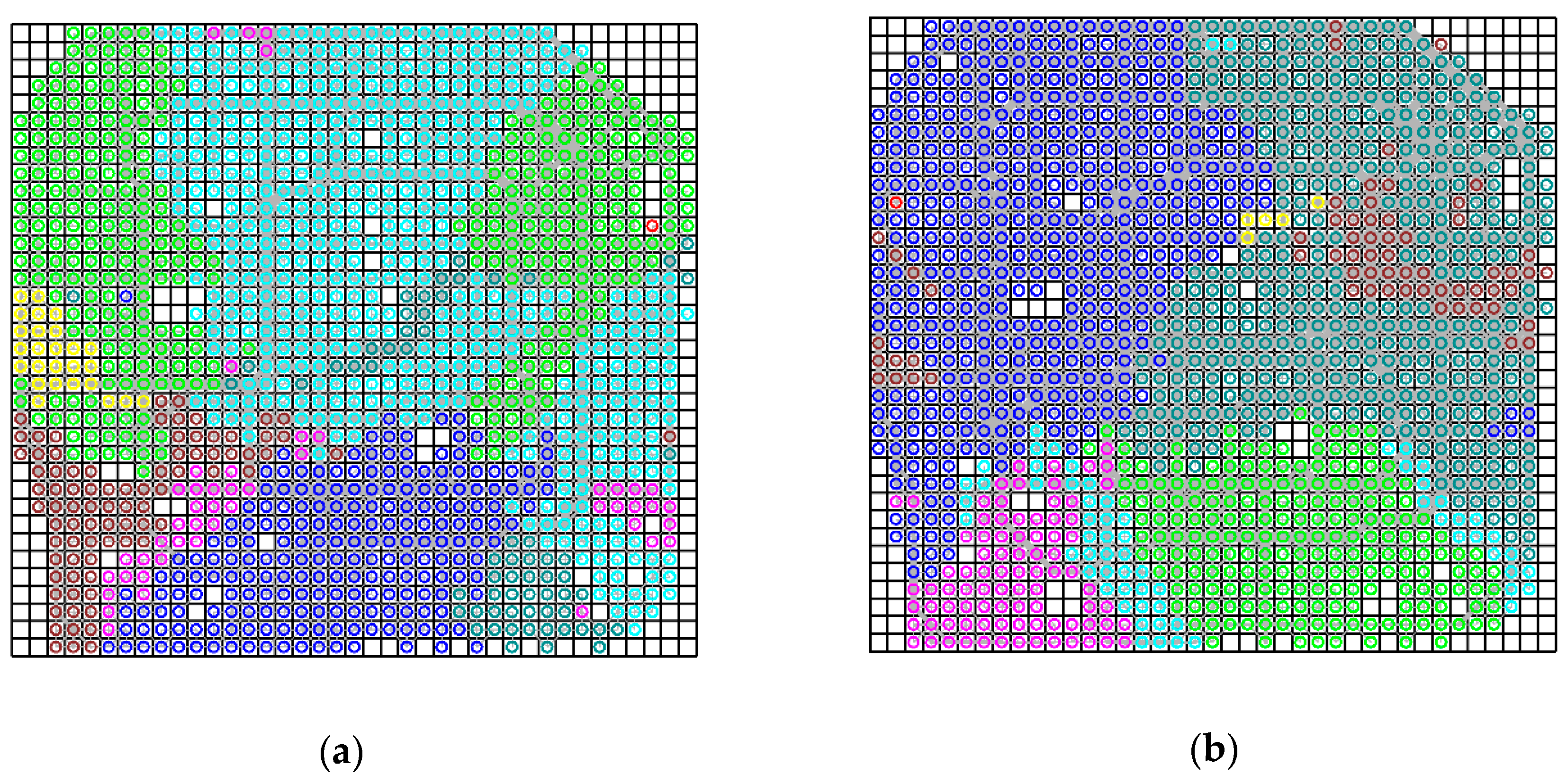
Besides the connectivity property, the spatially embedded network can also imply the aggregation patterns of land uses in the functional space. The land uses that have a strong connectivity relationship in the network traffic flow tend to be grouped together (Figure 7), and, in this way, we can explore the city structure and transport system using the resulting clustering patterns of land uses.

As presented in Figure 7, we classified the land uses into eight communities and there were some cells with no nodes. This is because there were no trajectory flows traversing across these cells. In addition, the land uses in the same community do not have to be contiguous in space. The reason is that our study aimed to cluster land uses from the perspective of their transport function, and the final similarity of the nodes was decided by both their attractive degree and structure similarity, which were calculated based on the spatially embedded network. Some neighboring land uses could have a low similarity due to their weak connectivity in the spatially embedded network, and some distant land uses could be grouped together if they are connected by a route with large traffic flows.

More specifically, as presented in Figure 7a, the study region in the morning rush hour was partitioned into five main communities, in each of which the land uses had a strong transport connection. Such relations also imply the actual aggregation of human activities and urban functions, e.g., the business district in the eastern part, the residential area in the southern part, and the universities in the northern area. In addition, there were four main communities in the noon rush hour. The most significant feature in this time period was that many communities were non-contiguous, or spanned multiple regions. For example, the community labeled by blue dots spanned the northern area (i.e., universities and high-technology regions) and the southern area (i.e., business districts and railway stations). In this time period, the traffic connection between distant land uses became stronger and cross-regional human activities were more frequent. In the period of the evening rush hour, the city was partitioned into two main communities which correspond to interactions among the residential areas, business districts, and universities. The small part (pink dots) corresponded to the connection between residential areas and train station areas. At midnight, there were four main communities, in which the large volume of traffic flows was directed for entertainment (e.g., bar). For example, the central Hohai entertainment area (green dots) attracted most of the neighboring land uses.

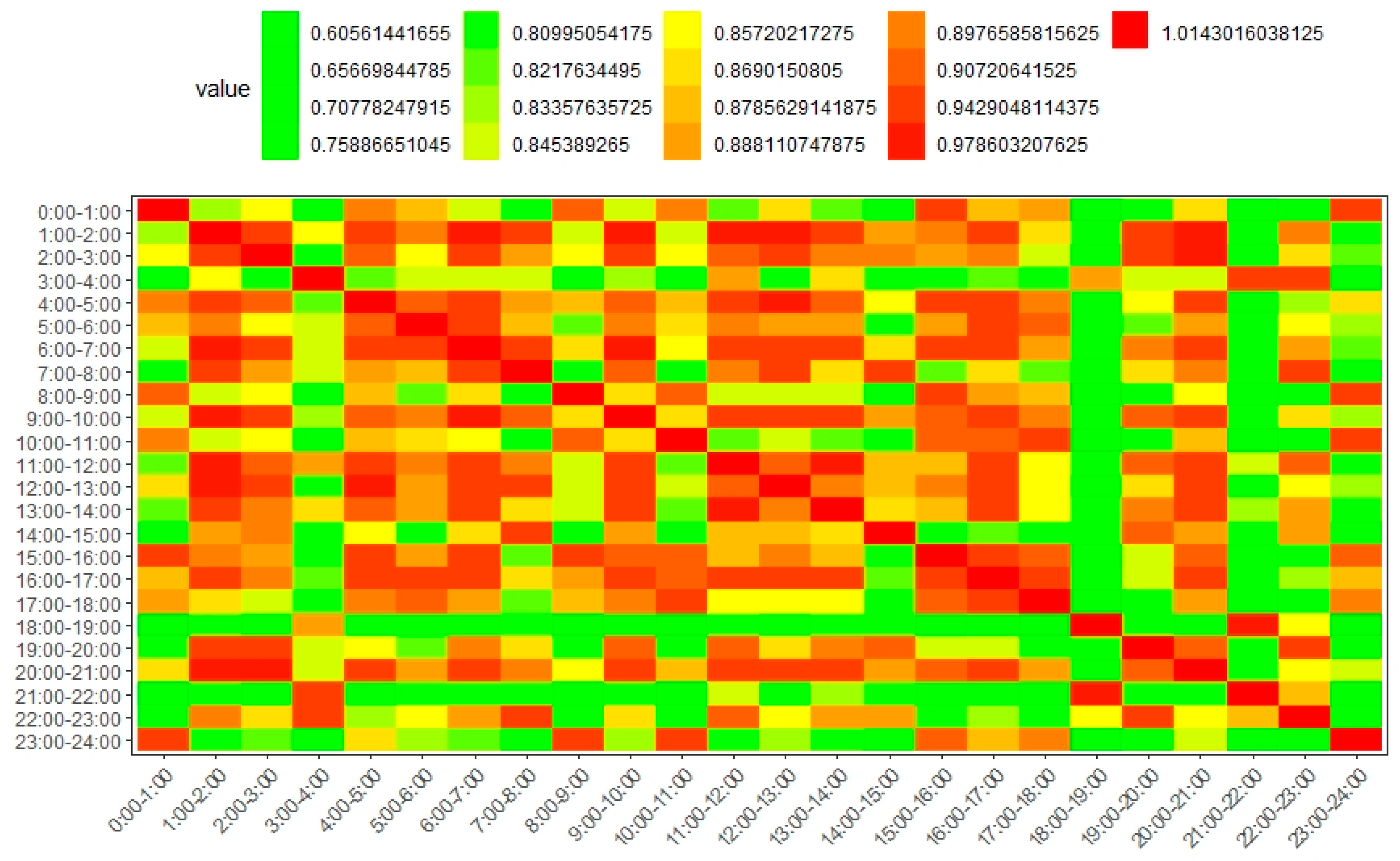
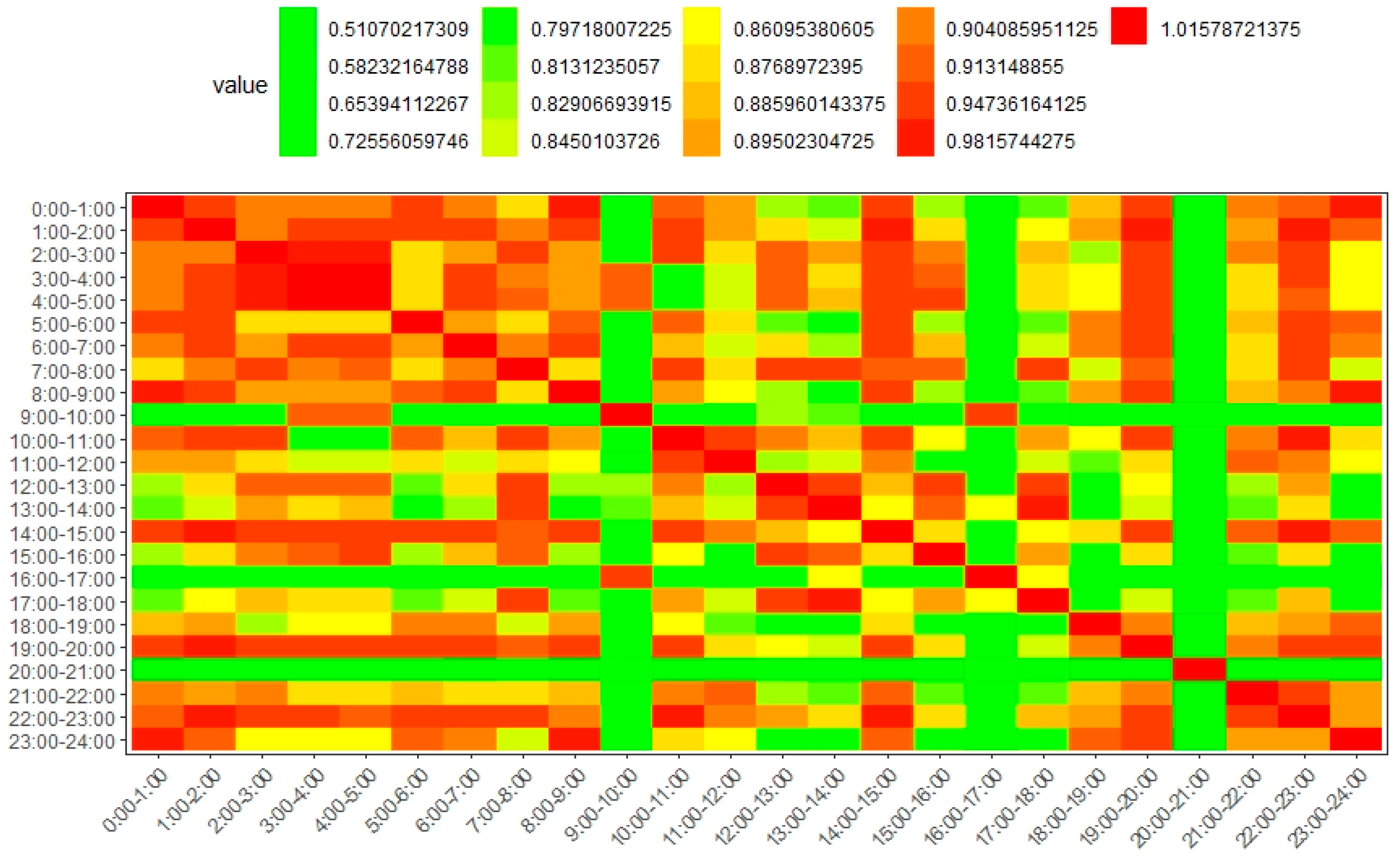
We then used the GSMM method to quantify the similarity between community structures in different time periods. In such a way, we were able to find out the degree to which the transport system changed across time. As presented in Figure 8, the GSMM measure values were calculated at the macro level rather than the micro level. First, it can be observed that community structures in successive time periods usually had a high similarity. For example, the community similarities in the successive time slices of [4:00–8:00], [11:00–14:00], and [15:00–18:00] were higher than those in non-successive time slices. Secondly, most of the community structures in the rush hours (e.g., the similarity between [7:00–8:00] and [8:00–9:00]) had a high similarity. Hence, the distributions of traffic flows are so regular in these periods that urban planners could estimate the associated travel behavior patterns. Note that the community structures between [12:00–14:00] and [4:00–7:00] were similar at the macro scale. Considering the routines and habits of residents, there are relatively few traffic flows in these periods and the arterial roads provide the main functions of transportation in the city. The travel origins and destinations are concentrated in a few business districts and railway stations. Hence, the traffic conditions in these time periods showed a similar characteristic. In addition, it can be observed that the community structure in [21:00–22:00] was very different from most of the structures in the other time periods. The reason may be that there are many different activities happening (e.g., working and entertainment) in [21:00–22:00], and thus the connectivity between local regions is much more complex than those in other time periods. Furthermore, the community structure in the evening rush hour of [18:00–19:00] was also very different from most of the other structures. This could be because in this time period the travel activities become increasingly active, and most of the residents in Beijing choose to travel along different routes. The land uses were also aggregated into different communities in this period compared to those in the successive time periods.

4.2. Variation in Different Spatial Scales

Our proposed method is adaptive to applications with different spatial scales. Hence, the next experiment refined the tessellation of space using a 500 m grid and analyzed the associated spatial community patterns across space and time.

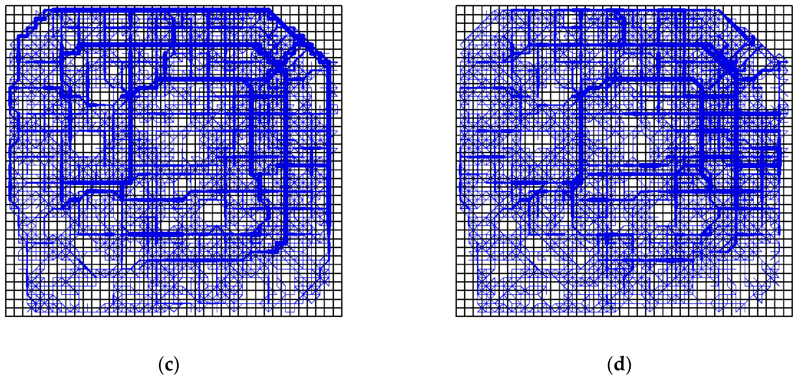
As the size of cells becomes smaller, there are more cells with no nodes, which correspond to the buildings (e.g., Imperial Palace) or lakes (e.g., Beihai Park) (Figure 9). We can easily observe the distributions of these land uses from the spatially embedded networks. In addition, compared to networks with 1000 m cell size, networks with 500 m cell size can present more detailed structures of street network infrastructure and associated traffic flows in the city. With the refined tessellation, we could observe more detailed interactions from the results. In the morning rush hour, strong connectivity existed mainly among the regions of residential areas, business districts, and high-tech areas. Entering the noon rush hour, the ring-like structure of the transport system became most significant. In addition, in the periods of the evening rush hour and midnight, the traffic flows were concentrated in the eastern and northern parts, which are the business cores of the city. Therefore, the transport system of Beijing depends largely on the loop lines, with a significant temporal pattern.

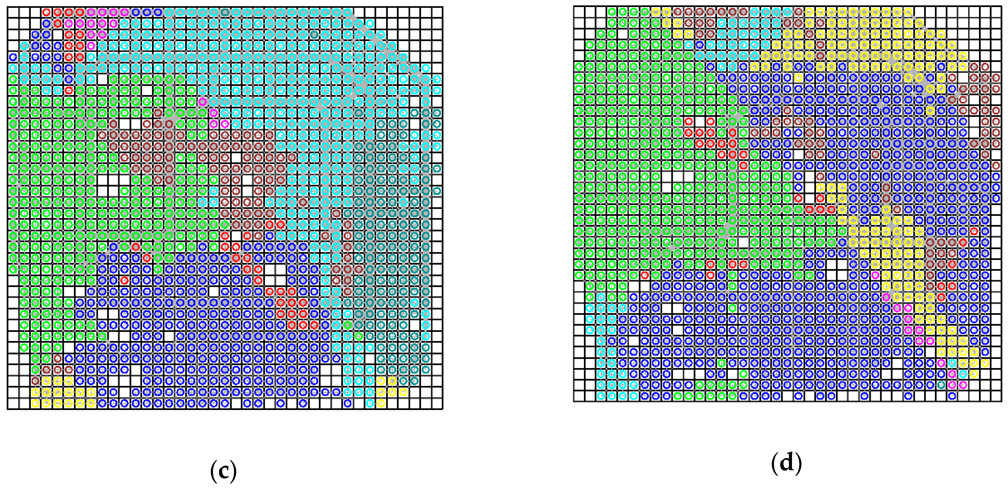
In order to compare the results under the two scales, we also classified the land uses into eight communities. As presented in Figure 10a, the study region was partitioned into three main communities in the morning rush hour. The eastern region was divided into two parts, and the community represented by green dots implies the aggregation of residential area (i.e., western part) and commercial business districts (i.e., eastern part). Another part in the eastern region was merged with the northern region, and the resulting community implies the aggregation of residential areas, universities, and high-technology regions. Later, entering the noon rush hour and the evening rush hour, the study region was partitioned into three communities and four communities, respectively. In addition, the aggregation of regions in both of the two time periods seems to be more significant than those in the corresponding time periods with cell size 1000 m. At midnight, the study area was partitioned into three communities. Compared to the result with cell size 1000 m, the interaction between land uses was weakened at midnight with cell size 500 m, and the region was divided into two main parts: one part was merged into the community of the business district (green dots), and the other one was merged into the community of business district and residential areas (blue dots). In general, the communities with cell size 500 m can reveal more detailed information of aggregation of land uses.

Using the GSMM method, we also calculated the similarity matrix, as presented in Figure 11. It can be observed that in the rush hours, the measured values with 500 m cell size were similar to those with 1000 m cell size. In addition, during the non-rush hours, the measured values with 500 m cell size were higher than the corresponding values with 1000 m cell size. The reason could be that, with the refining of space tessellation, more cells had traffic flows and the number of the matching cells across time increased. Specifically, the small size grid can capture the local interactions between regions, which were more regular in the non-rush hours than in the rush hours (see Figure 9).

4.3. Algorithm Efficiency with Different Cell Sizes

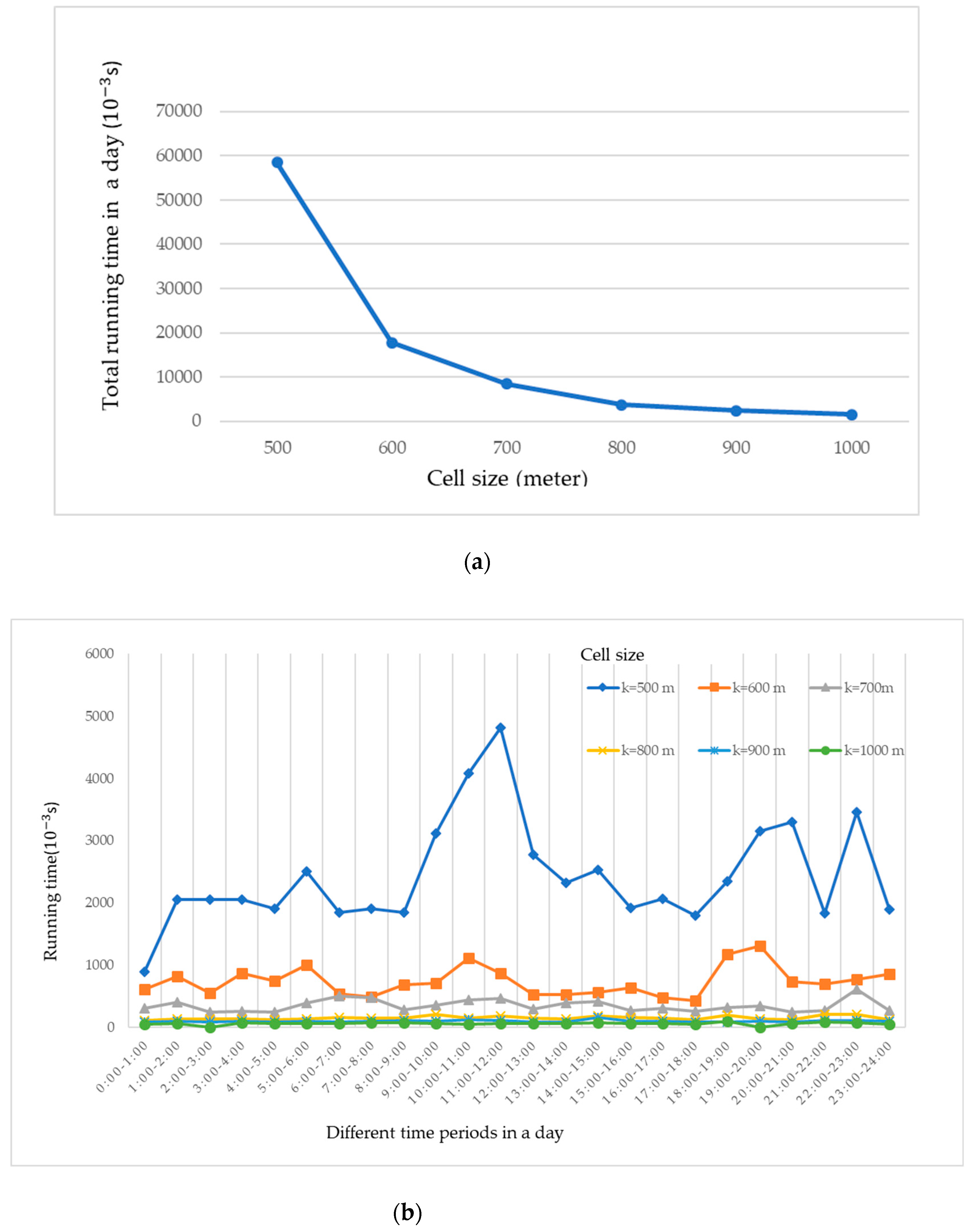
The results above show the effect of different cell sizes on community detection. In order to further explore the algorithm efficiency with different cell sizes, we implemented the method with cell sizes of 500 m, 600 m, 700 m, 800 m, 900 m, and 1000 m.

With the increase of cell size, the total running time decreased (Figure 12a), and when the cell size changed from 500 m to 700 m, the algorithm efficiency increased sharply. When the cell size changed from 700 m to 1000 m, the running time remained stable. The reason could be that the number of nodes decreased with the increase of cell size, and thus the algorithm cost less time during the clustering of nodes. Furthermore, when the cell size was larger than 700 m, the number of iterations in k-means algorithm did not change much, and thus the running time of the algorithm remained stable. In addition, as presented in Figure 12b, the running time of the algorithm changed across the time periods. In general, the running time of the algorithm in the rush hours (e.g., 7:00–9:00, 11:00–13:00, 18:00–20:00, 22:00–23:00) was larger than those in the other hours. The reason could be that the flow structures are more complex in rush hours.

5. Conclusion and Future Directions

Based on the collective intra-city trips extracted from the emerging taxi GPS trajectory data, this paper explored network traffic flows towards a deep understanding of city structure. We introduced network science techniques (e.g., community detection) to reveal the regular patterns of traffic flows across space and time. More specifically, aiming at the connectivity, aggregation, and dynamic properties of transport system, we proposed a three level framework to explore the complex traffic network. It firstly partitions the study region and constructs a spatially embedded network for representing the connectivity relationships between local regions. In order to extract the aggregation patterns of land uses, the method then uses the community detection techniques based on the volume of traffic flows and structural properties of the network. Furthermore, our method employs a graph structure matching measure to uncover the regularities of the transport system across time. The proposed method is also adaptive to multi-scale applications in space and time.

Through the case study, we found that the interactions of land uses show different characteristics in different time periods, and the aggregation patterns of functional areas is dynamic across the time. This result is highly associated with the travel behaviors of residents in the city, and thus can be used further in social science research. In addition, the result can provide references for the dispatching of the traffic system. For example, we can plan for the prevention of traffic jams in regions which have intense interactions of traffic flows. Moreover, it can be used to assist urban structure analysis. As presented in our case study, Beijing has a polycentric form with significant loop structure.

In this paper, we took the taxi trajectory data into consideration because taxi accounts for a large proportion of public transport in Beijing city. Taxi drivers are very familiar with the city of concern, and thus there are increasingly more studies focusing on the use of taxi trajectory data for urban analysis [3,12,33]. In addition, since the taxi is a common mode of transport, our method could be adaptable to other cities. We would like to regard this research as a beginning of detecting spatial interaction communities based on vehicle datasets. With the rapid development of big data, more traffic data (e.g., bus trajectories, passenger car data, and biking trajectories) can be introduced into our framework for exploring city structures comprehensively. Further study can also use more methods (e.g., complex system) to understand the mechanisms of the traffic flow space. It would be interesting to analyze the associations between the physical space and virtual space of a city using social media data.