Tarantula: Design, Modeling, and Kinematic Identification of a Quadruped Wheeled Robot

 , and
, and
Abstract
:1. Introduction
- Design of the robotic platform that can change its height and is holonomic,
- Formulation for kinematics of the wheeled locomotion coupled with the leg kinematics,
- Identification of kinematic parameters after the assembly of the robot, using monocular vision and ArUco markers,
- Trajectory tracking of the robot using the same set-up of monocular vision and ArUco markers.
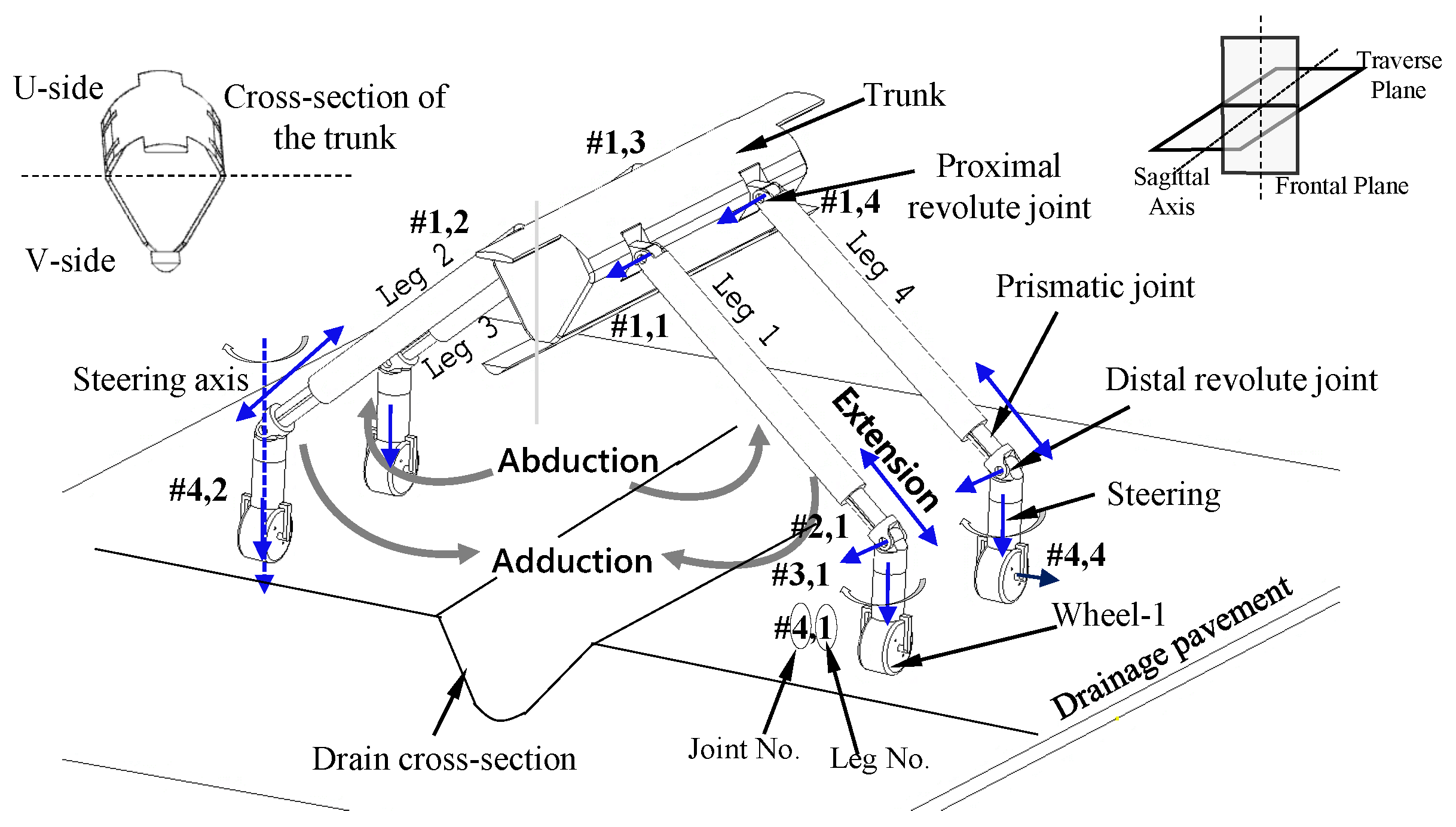
2. Robot Architecture
2.1. Design Requirements
- The robotic system should have the capability to move around inside the drain environment. Hence, it must be mobile, unlike fixed industrial robots.
- The mobile platform should reconfigure its height as per the geometry of the drainages (Figure 1)
- The mobile robot should be able to manoeuvre the sharp angular turns inside the drains with minimum turning radius.
- The robot should be modular so that the components can be replaced easily in case of damage.
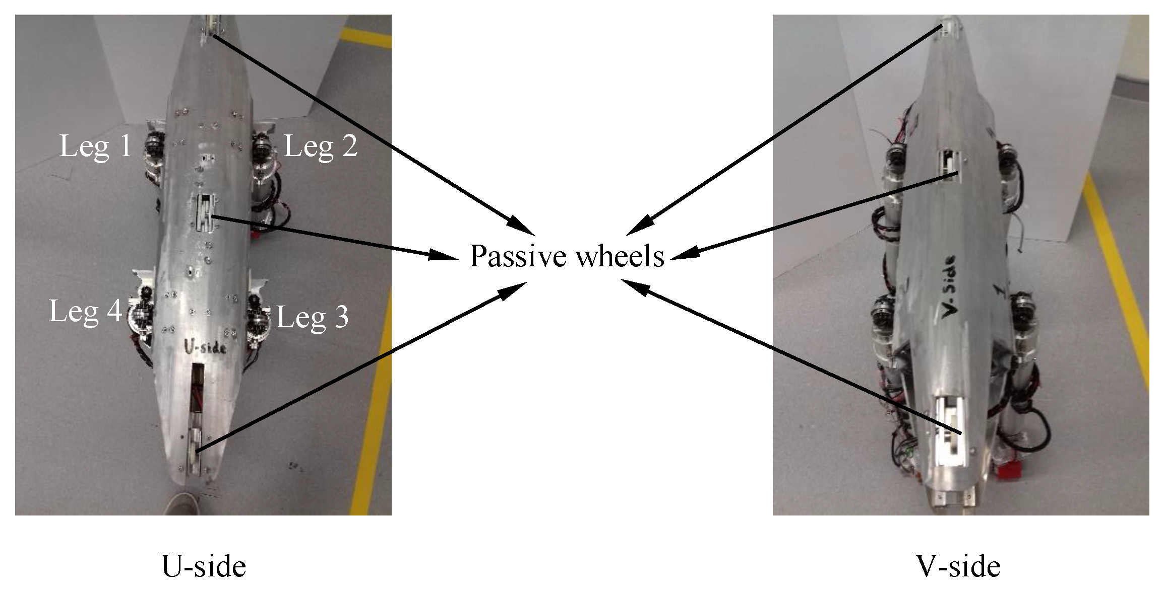
2.2. Mechanical Layout
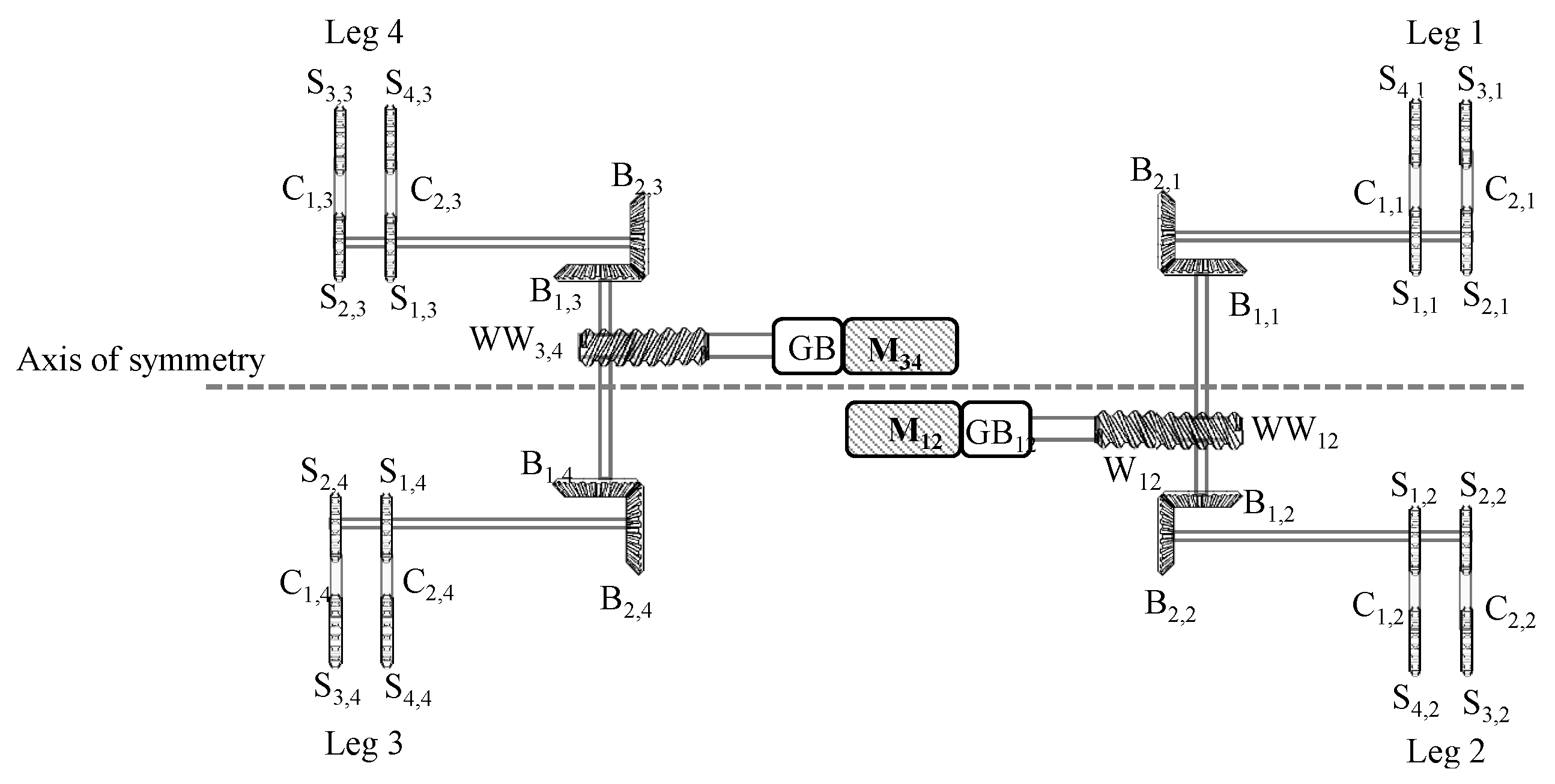
2.2.1. Trunk
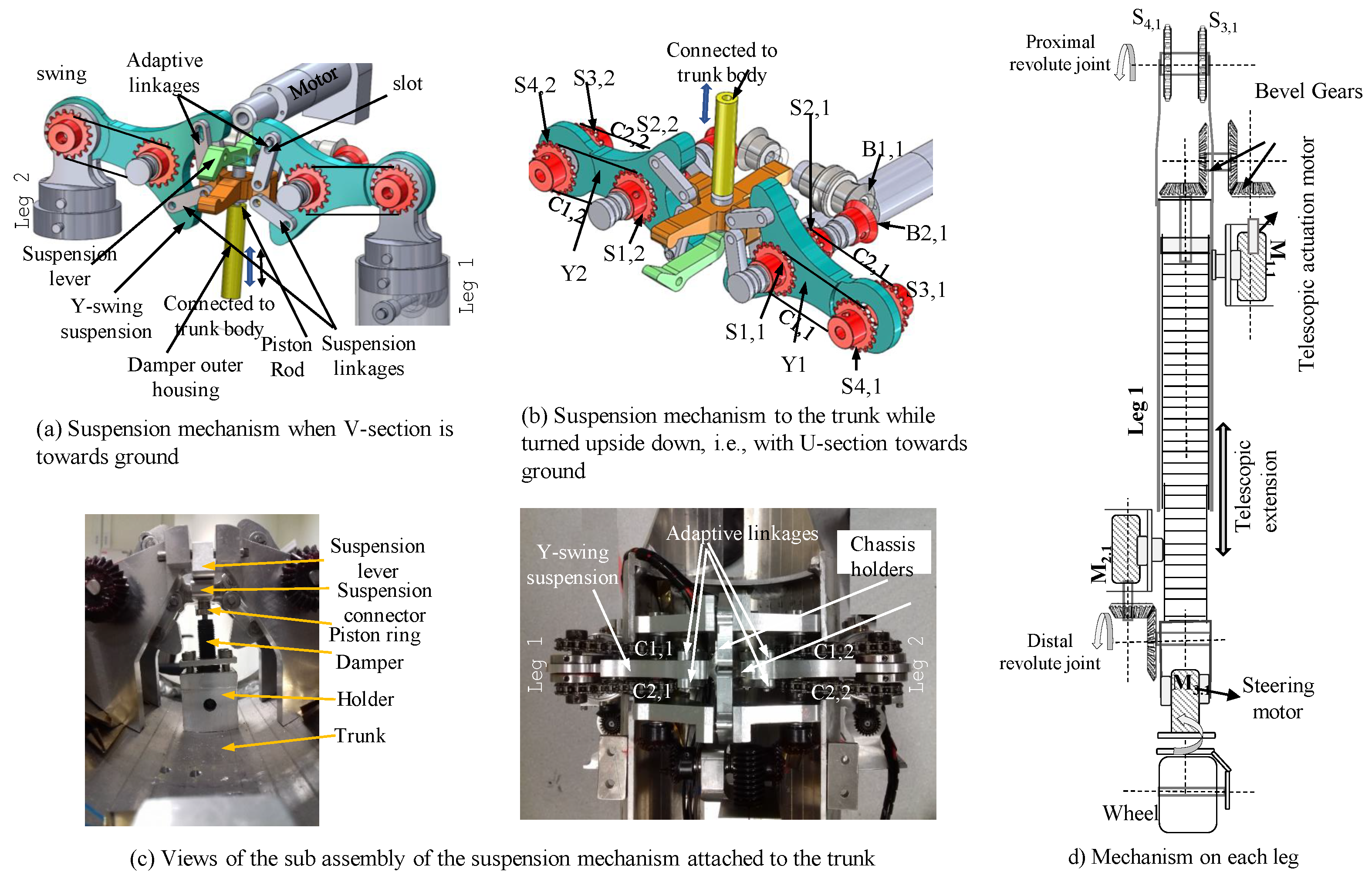
2.2.2. Telescopic Extension and Distal Revolute Joint
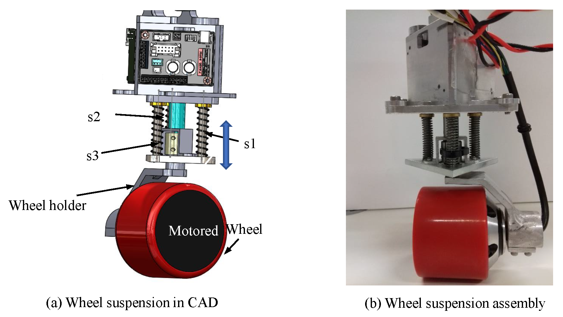
2.2.3. Steering and Wheel Suspension
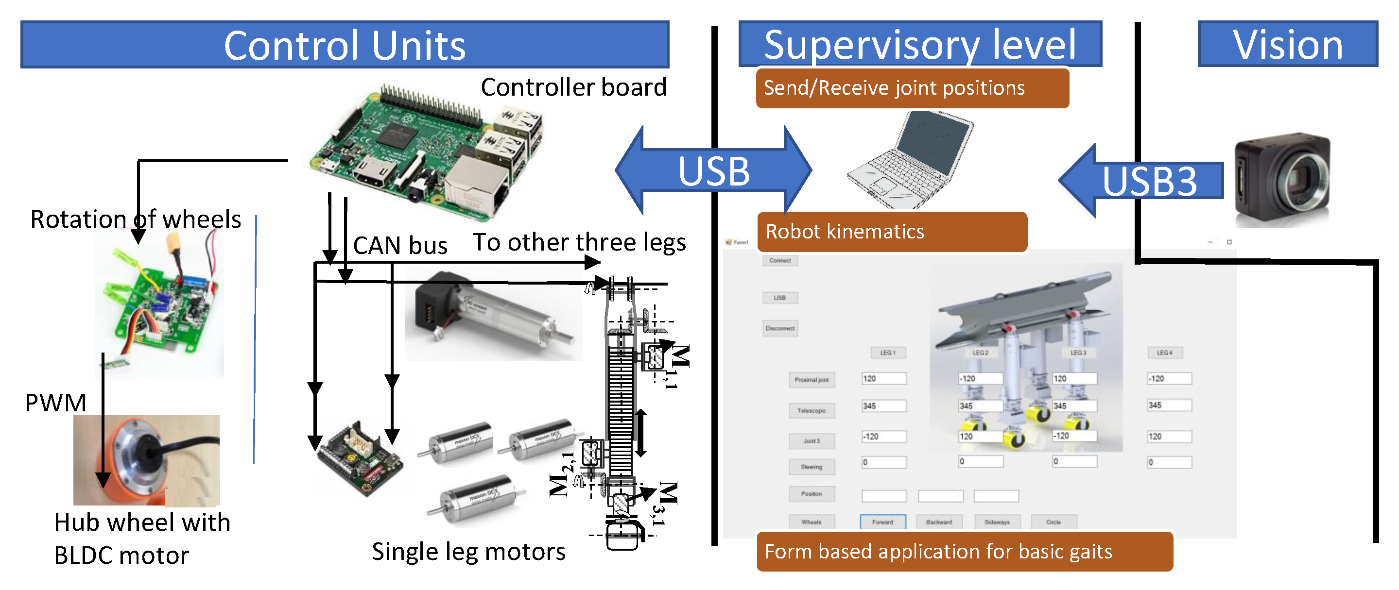
2.2.4. Tarantula Electronics
3. Modeling and Simulation
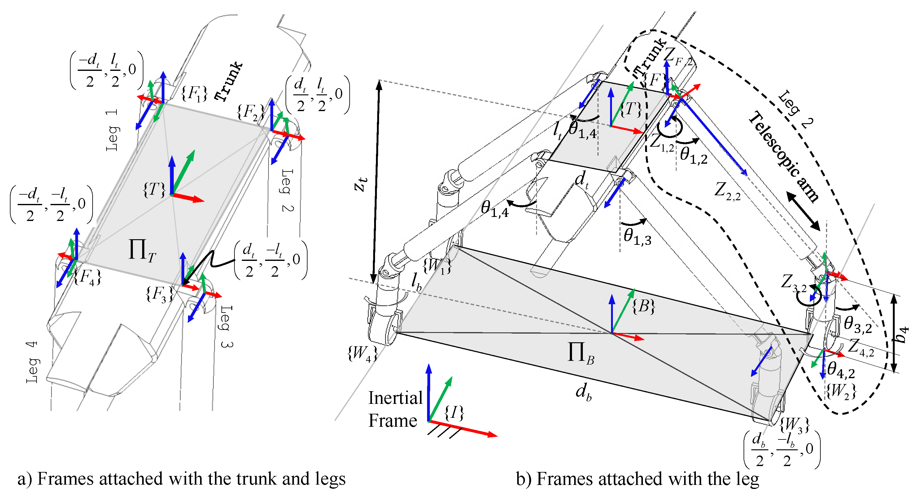
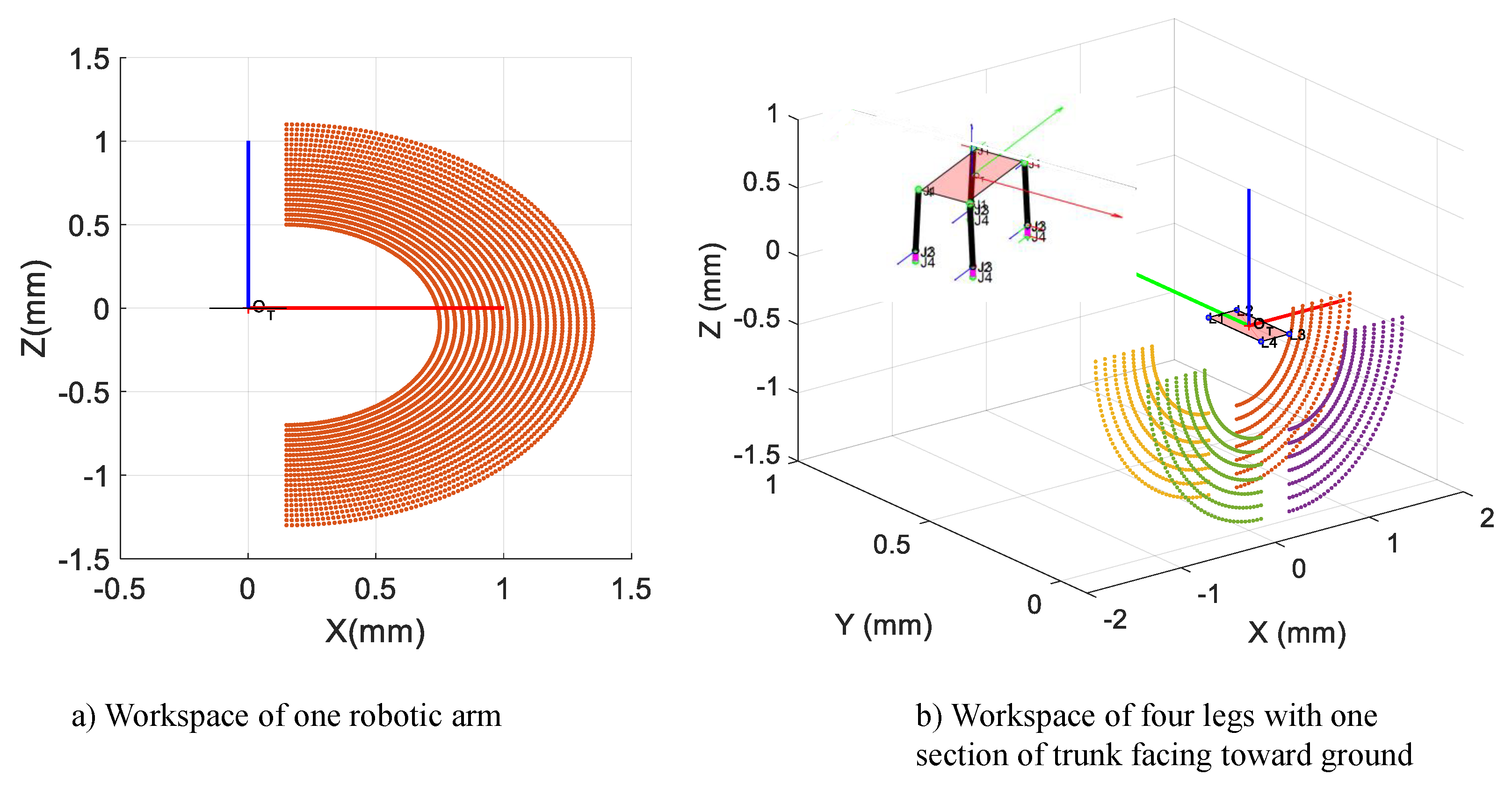
3.1. Kinematic Modeling
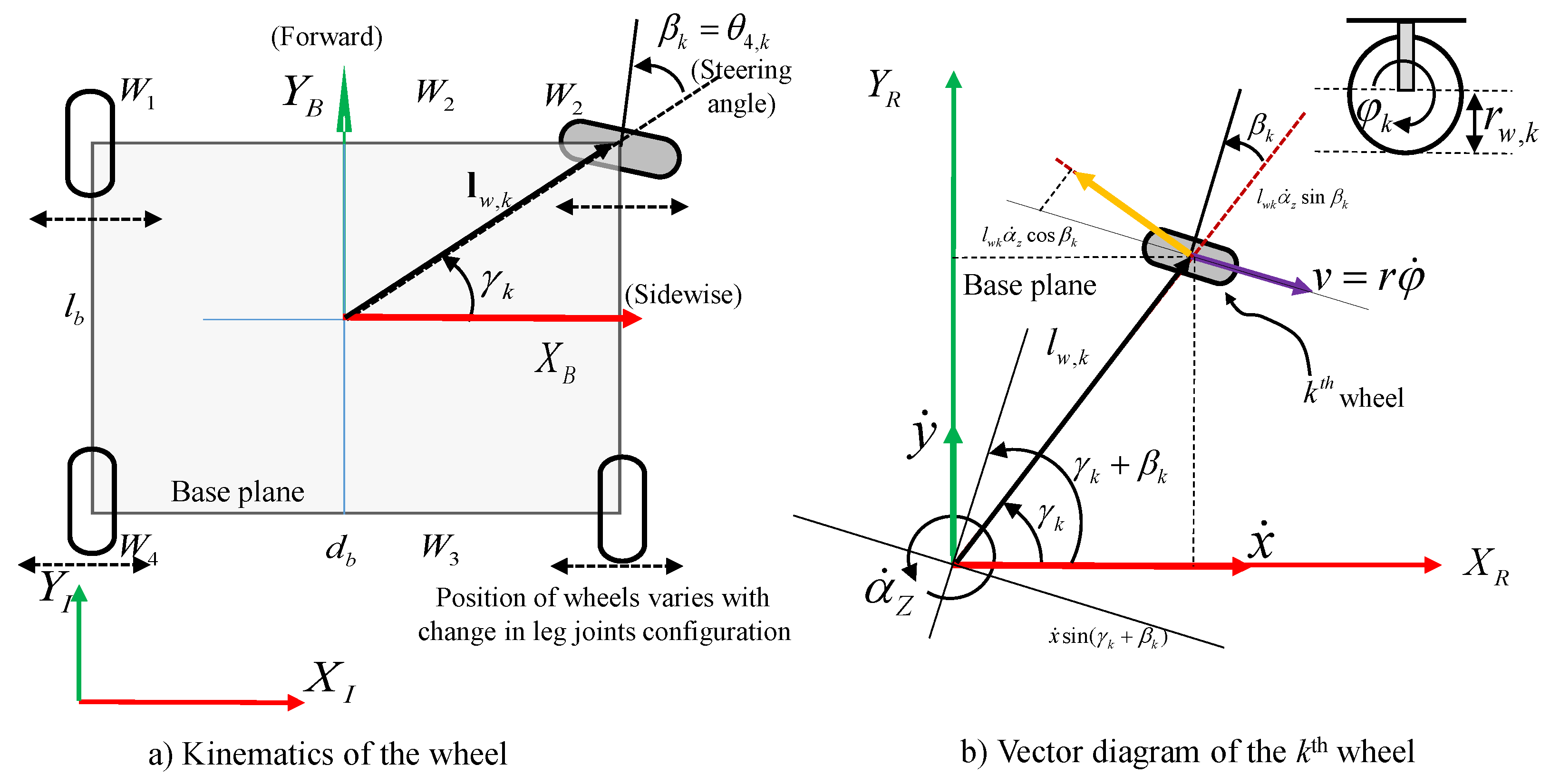
3.2. Kinematics of Wheel
4. Experiments
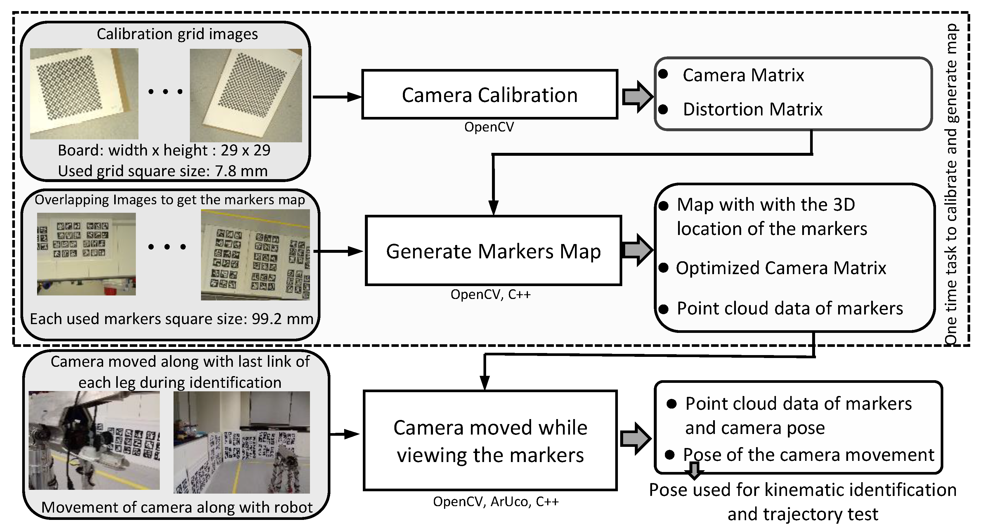
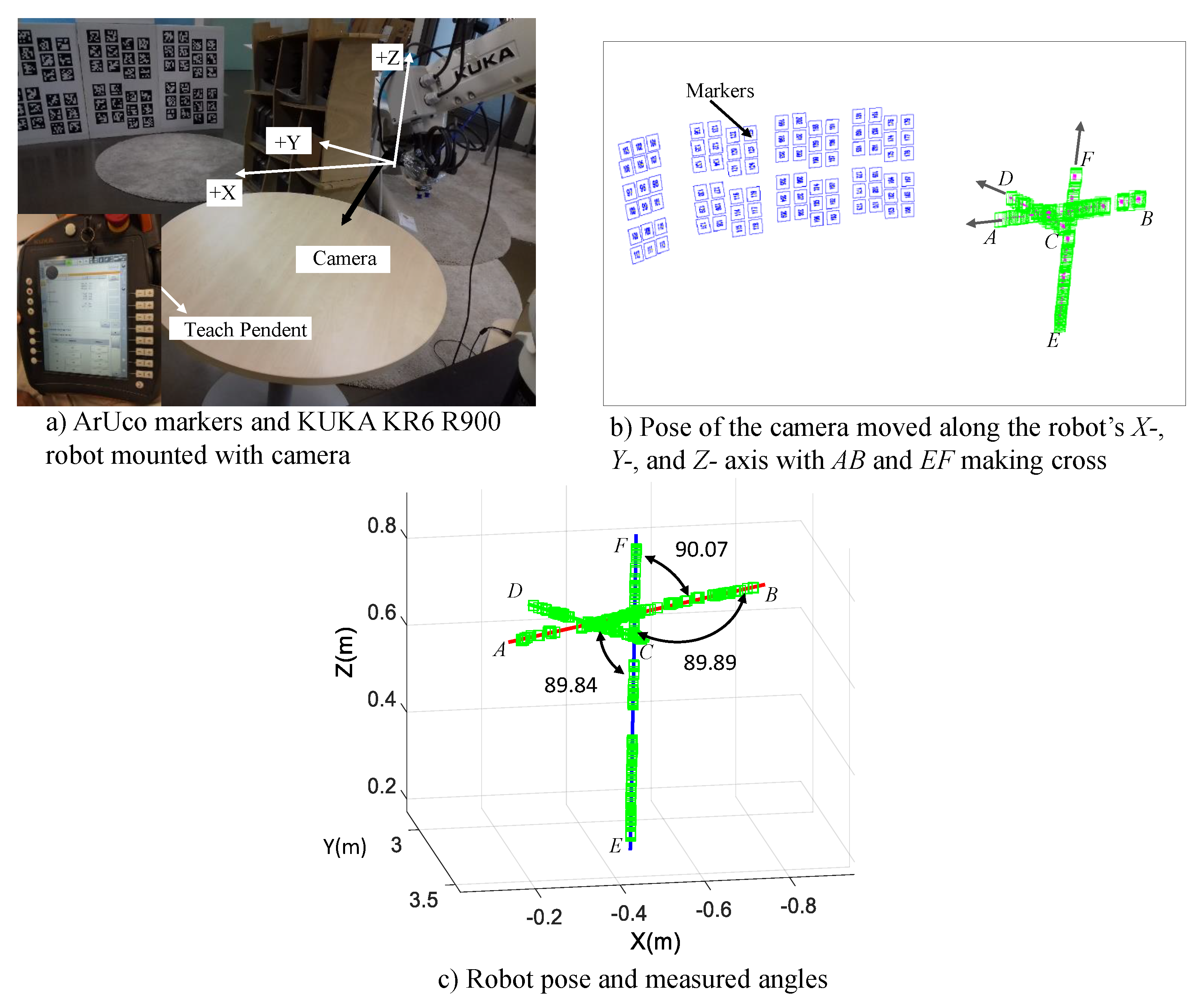
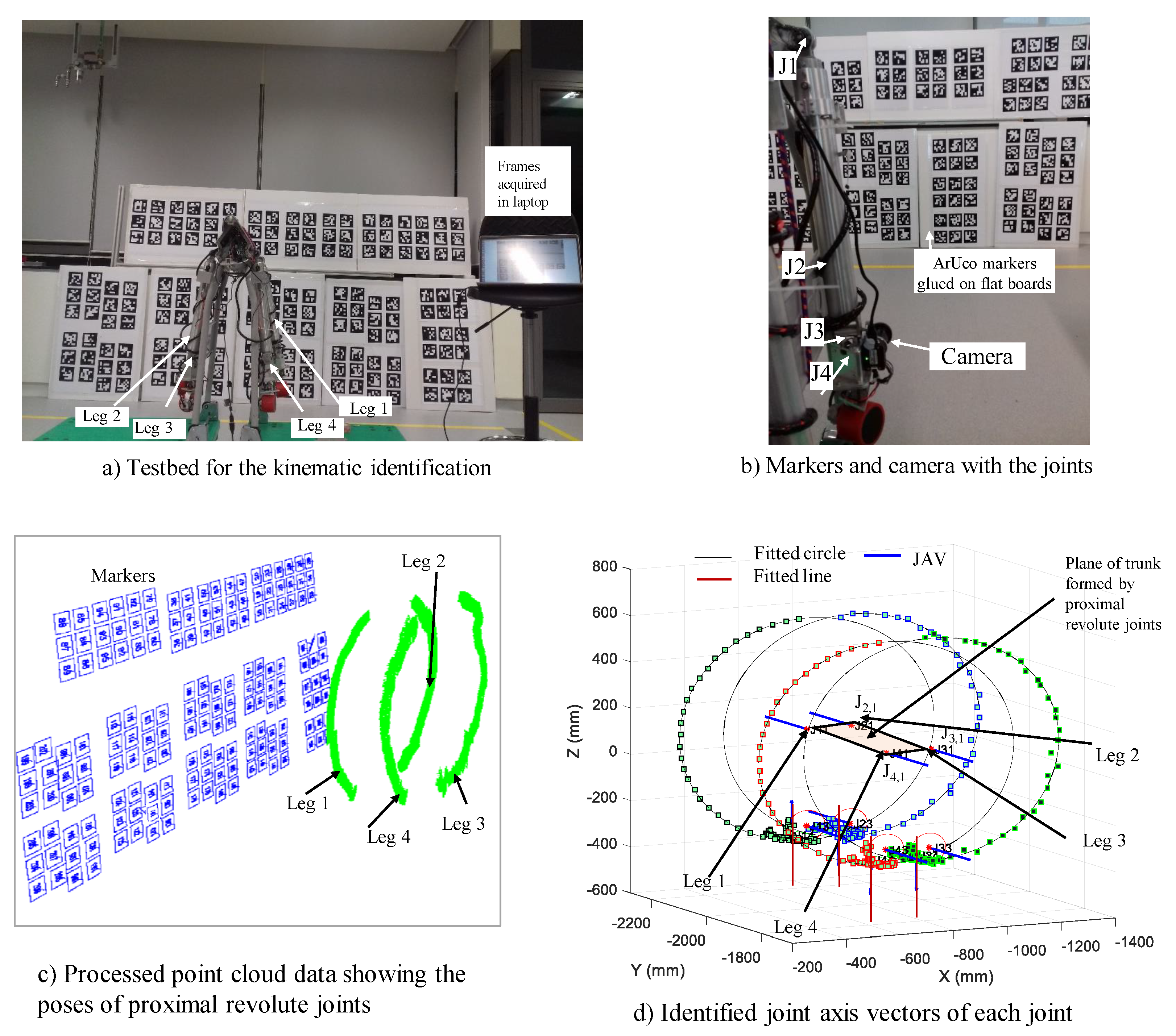
4.1. Setup
4.2. Measurement Performance
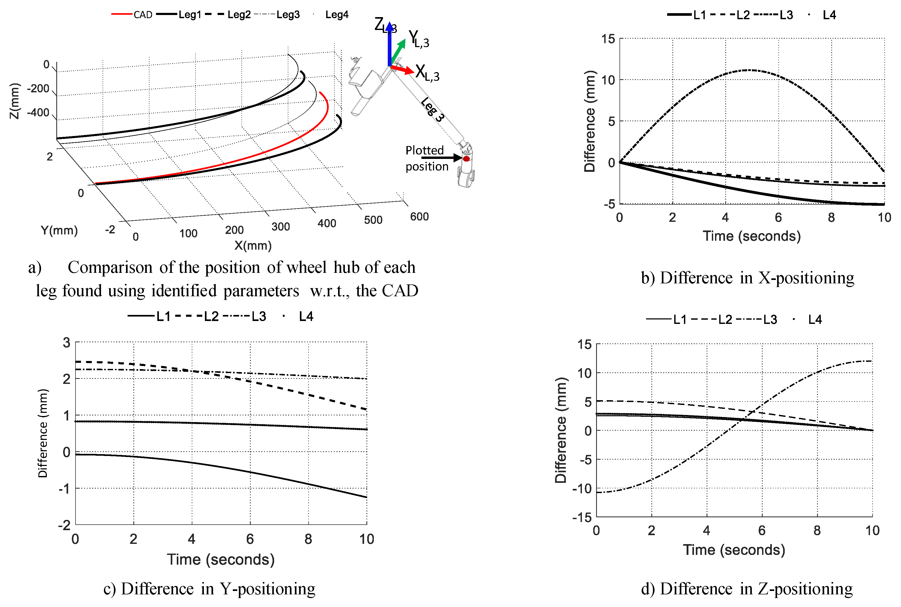
4.3. Identification of Kinematic Parameters of Tarantula
| Algorithm 1 Algorithm to find the Denavit–Hartenberg (DH) parameters. | |
| – Fix the camera on the last link of the legged robot and keep the trunk fixed, (as shown in Figure 14b). | |
| Fori = 1 to n | |
| – Move one joint at a time starting from the first joint while locking the rest. The position of the camera will trace the circular arc and prismatic joint will trace a straight line. | |
| – Log the 3D positions of the camera using ArUco markers map set-up (Section 4). For revolute joint actuate it by and record the video feed from the camera with aruco markers visible, while for the prismatic joint it was actuated by distance l. | |
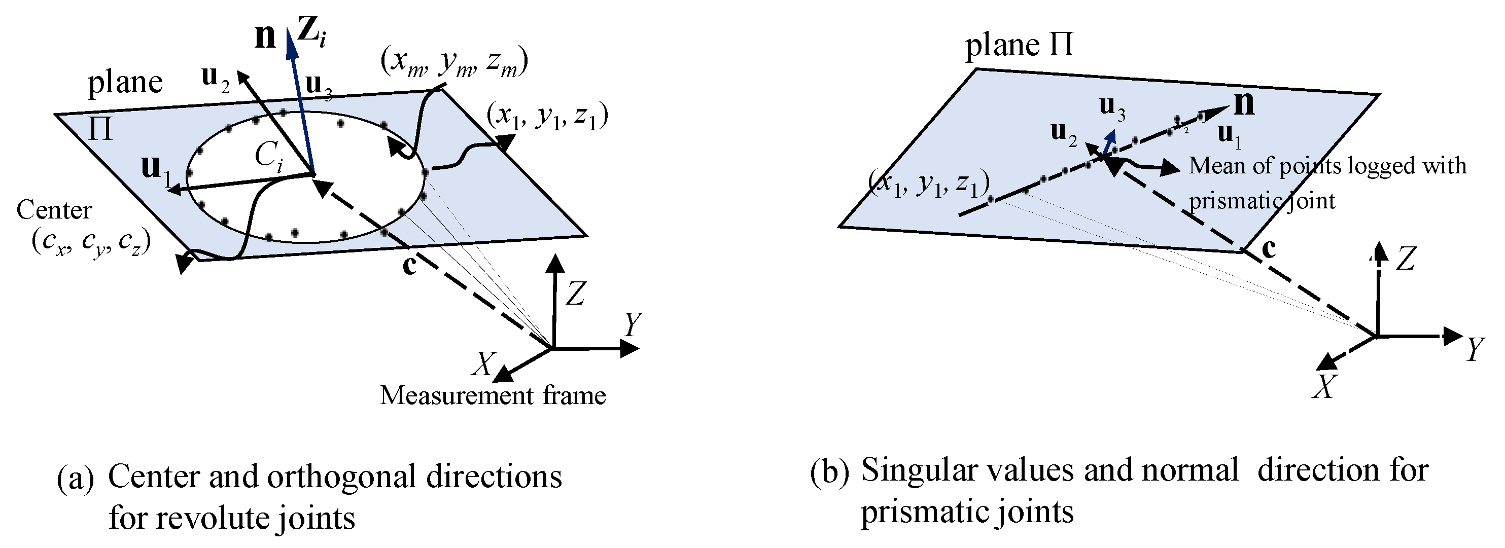
| – Find the centre of the circle using 3D circle fitting method for revolute joints and mean of linear points for prismatic joints with the direction of joint axis vector as the normal of the plane of movement. | |
| End for | |
| For to 1 | |
| Extract the DH parameters, i.e., , and , using JAVs as inputs to find the perpendicular distances and angles between the two successive joint axis vectors. | |
| End for | |
| – Repeat the above steps for each leg. | |
| – With the coordinates of center of rotation of proximal joints, estimate the effective dimension of the plane of trunk as shown in Figure 8. | |
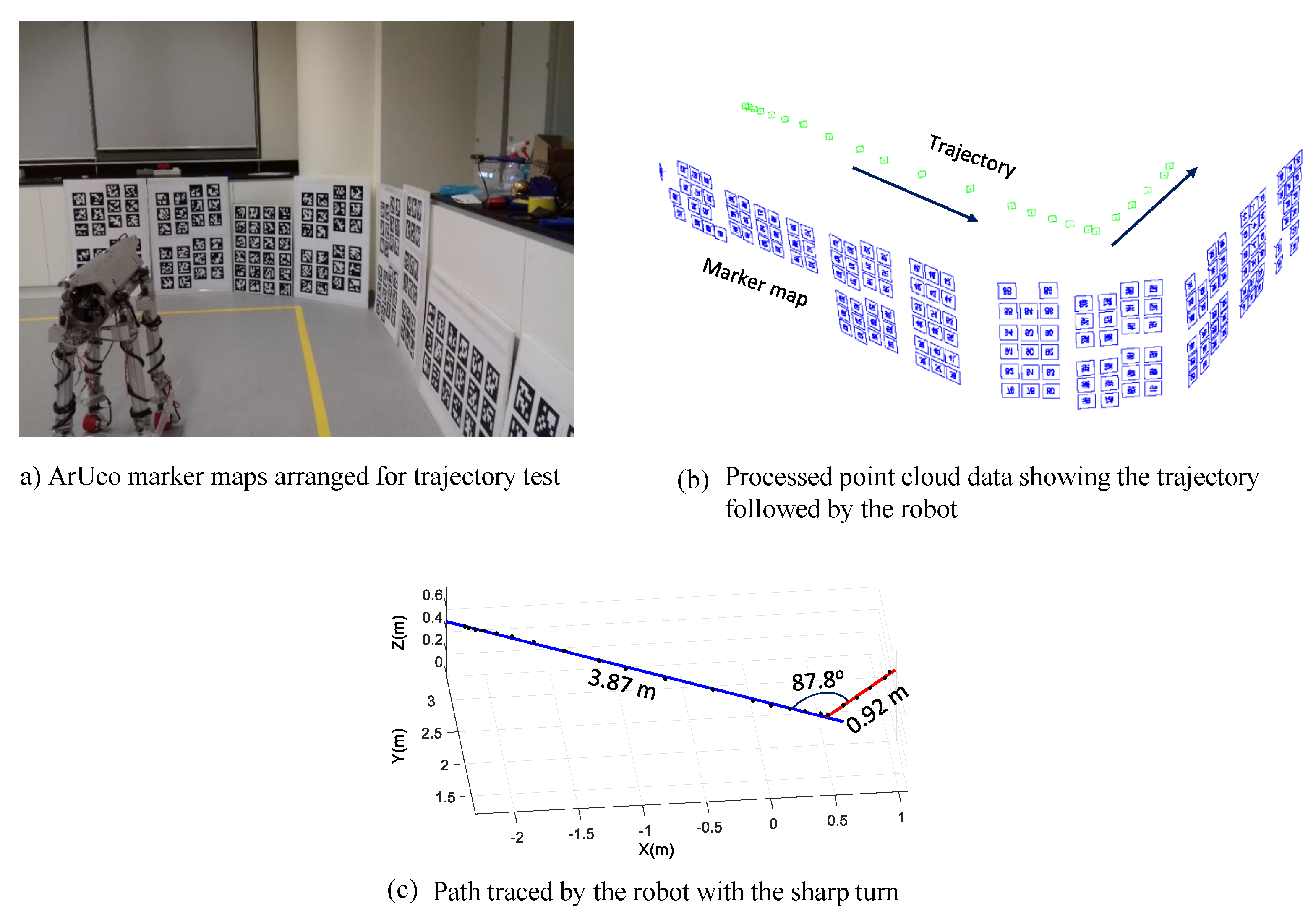
4.4. Trajectory Tracking
5. Conclusions and Future Works
- Design of the modular robot Tarantula with the ability to reconfigure its height, mainly for inspecting the drains,
- A mechanism designed for the simultaneous abduction/adduction of legs,
- A methodology to identify the kinematic parameters using ArUco markers and monocular vision for the assembled mobile robot with legs. First, using the calibrated camera, poses of ArUco markers are reconstructed in 3D space. Second, by moving each joint and capturing images, a set of the tracked pose is determined. Then, the DH parameters were evaluated.
Author Contributions
Funding
Conflicts of Interest
Appendix A. DH Parameters Notation Used [48]


| Parameters (Name) | Description * |
|---|---|
| b (Joint offset) | |
| θ (Joint angle) | |
| a (Link length) | |
| α (Twist angle) |
References
- Zhang, S.X.; Pramanik, N.; Buurman, J. Exploring an innovative design for sustainable urban water management and energy conservation. Int. J. Sustain. Dev. World Ecol. 2013, 20, 442–454. [Google Scholar] [CrossRef]
- Kirkham, R.; Kearney, P.D.; Rogers, K.J.; Mashford, J. PIRAT—A system for quantitative sewer pipe assessment. Int. J. Robot. Res. 2000, 19, 1033–1053. [Google Scholar] [CrossRef]
- Bradbeer, R. The Pearl Rover Underwater Inspection Robot. In Mechatronics and Machine Vision; Billingsley, J., Ed.; Research Studies Press: Baldock, UK, 2000; pp. 255–262. [Google Scholar]
- Truong-Thinh, N.; Ngoc-Phuong, N.; Phuoc-Tho, T. A study of pipe-cleaning and inspection robot. In Proceedings of the International Conference on Robotics and Biomimetics (ROBIO), Karon Beach, Phuket, Thailand, 7–11 December 2011; pp. 2593–2598. [Google Scholar]
- Kuntze, H.; Schmidt, D.; Haffner, H.; Loh, M. KARO-A flexible robot for smart sensor-based sewer inspection. In Proceedings of the No Dig’95, Dresden, Germany, 19–22 September 1995; pp. 367–374. [Google Scholar]
- Nassiraei, A.A.; Kawamura, Y.; Ahrary, A.; Mikuriya, Y.; Ishii, K. Concept and design of a fully autonomous sewer pipe inspection mobile robot KANTARO. In Proceedings of the International Conference on Robotics and Automation, Roma, Italy, 10–14 April 2007; pp. 136–143. [Google Scholar]
- Kirchner, F.; Hertzberg, J. A prototype study of an autonomous robot platform for sewerage system maintenance. Auton. Robots 1997, 4, 319–331. [Google Scholar] [CrossRef]
- Streich, H.; Adria, O. Software approach for the autonomous inspection robot MAKRO. In Proceedings of the International Conference on Robotics and Automation, New Orleans, LA, USA, 26 April–1 May 2004; Volume 4, pp. 3411–3416. [Google Scholar]
- Baghani, A.; Ahmadabadi, M.N.; Harati, A. Kinematics modeling of a wheel-based pole climbing robot (UT-PCR). In Proceedings of the 2005 IEEE International Conference on Robotics and Automation (ICRA 2005), Barcelona, Spain, 18–22 April 2005; pp. 2099–2104. [Google Scholar]
- Ratanghayra, P.R.; Hayat, A.A.; Saha, S.K. Design and Analysis of Spring-Based Rope Climbing Robot. In Machines, Mechanism and Robotics; Springer: Berlin, Germany, 2019; pp. 453–462. [Google Scholar]
- Fuchida, M.; Pathmakumar, T.; Mohan, R.E.; Tan, N.; Nakamura, A. Vision-based perception and classification of mosquitoes using support vector machine. Appl. Sci. 2017, 7, 51. [Google Scholar] [CrossRef]
- Raibert, M.H. Legged Robots That Balance; MIT Press: Cambridge, MA, USA, 1986. [Google Scholar]
- Berns, K.; Ilg, W.; Deck, M.; Albiez, J.; Dillmann, R. Mechanical construction and computer architecture of the four-legged walking machine BISAM. IEEE/ASME Trans. Mechatron. 1999, 4, 32–38. [Google Scholar] [CrossRef]
- Ridderstrom, C.; Ingvast, J. Quadruped posture control based on simple force distribution-a notion and a trial. In Proceedings of the International Conference on Intelligent Robots and Systems, Maui, HI, USA, 29 October–3 November 2001; Volume 4, pp. 2326–2331. [Google Scholar]
- Hirose, S.; Kato, K. Study on quadruped walking robot in Tokyo Institute of Technology-past, present and future. In Proceedings of the International Conference on Robotics and Automation, San Francisco, CA, USA, 24–28 April 2000; Volume 1, pp. 414–419. [Google Scholar]
- Kitano, S.; Hirose, S.; Endo, G.; Fukushima, E.F. Development of lightweight sprawling-type quadruped robot titan-xiii and its dynamic walking. In Proceedings of the International Conference on Intelligent Robots and Systems (IROS), Tokyo, Japan, 3–7 November 2013; pp. 6025–6030. [Google Scholar]
- Arikawa, K.; Hirose, S. Development of quadruped walking robot TITAN-VIII. In Proceedings of the IEEE/RSJ International Conference on Intelligent Robots and Systems (IROS 96), Osaka, Japan, 8 November 1996; Volume 1, pp. 208–214. [Google Scholar]
- De Santos, P.G.; Garcia, E.; Estremera, J. Quadrupedal Locomotion: An Introduction to the Control of Four-Legged Robots; Springer Science & Business Media: Berlin, Germany, 2007. [Google Scholar]
- Montes, H.; Armada, M. Force control strategies in hydraulically actuated legged robots. Int. J. Adv. Robot. Syst. 2016, 13, 50. [Google Scholar] [CrossRef]
- Li, T.; Ma, S.; Li, B.; Wang, M.; Li, Z.; Wang, Y. Development of an in-pipe robot with differential screw angles for curved pipes and vertical straight pipes. J. Mech. Robot. 2017, 9, 051014. [Google Scholar] [CrossRef]
- Sharf, I. Dynamic Locomotion with a Wheeled-Legged Quadruped Robot. In Brain, Body and Machine; Springer: Berlin, Germany, 2010; pp. 299–310. [Google Scholar]
- Barker, L.K. Vector-Algebra Approach to Extract Denavit–Hartenberg Parameters of Assembled Robot Arms; NASA Langley Research Center: Hampton, VA, USA, 1983.
- Hollerbach, J.M.; Wampler, C.W. The calibration index and taxonomy for robot kinematic calibration methods. Int. J. Robot. Res. 1996, 15, 573–591. [Google Scholar] [CrossRef]
- De Santos, P.G.; Jiménez, M.A.; Armada, M.A. Improving the motion of walking machines by autonomous kinematic calibration. Auton. Robots 2002, 12, 187–199. [Google Scholar] [CrossRef]
- Hayat, A.A.; Chittawadigi, R.; Udai, A.; Saha, S.K. Identification of Denavit-Hartenberg parameters of an industrial robot. In Proceedings of the Conference on Advances in Robotics, Pune, India, 4–6 July 2013; pp. 1–6. [Google Scholar]
- Denavit, J.; Hartenberg, R.S. A kinematic notation for lower-pair mechanisms based on matrices. Trans. ASME J. Appl. Mech. 1955, 22, 215–221. [Google Scholar]
- Driels, M.R.; Swayze, W.; Potter, S. Full-pose calibration of a robot manipulator using a coordinate-measuring machine. Int. J. Adv. Manuf. Technol. 1993, 8, 34–41. [Google Scholar] [CrossRef]
- Liu, B.; Zhang, F.; Qu, X.; Shi, X. A Rapid coordinate transformation method applied in industrial robot calibration based on characteristic line coincidence. Sensors 2016, 16, 239. [Google Scholar] [CrossRef] [PubMed]
- Babinec, A.; Jurišica, L.; Hubinskỳ, P.; Duchoň, F. Visual localization of mobile robot using artificial markers. Procedia Eng. 2014, 96, 1–9. [Google Scholar] [CrossRef]
- RobotWorx. Available online: https://www.robots.com/robots/kuka-kr-6-r900-fivve (accessed on 27 October 2018).
- Record Breaking Limbo Skater: 6-Year-Old Skates under 39 Cars—YouTube. Available online: https://www.youtube.com/watch?v=7HEPRZuRWvc (accessed on 1 July 2018).
- Kee, V.; Rojas, N.; Elara, M.R.; Sosa, R. Hinged-Tetro: A self-reconfigurable module for nested reconfiguration. In Proceedings of the 2014 IEEE/ASME International Conference on Advanced Intelligent Mechatronics (AIM), Besacon, France, 8–11 July 2014; pp. 1539–1546. [Google Scholar]
- Prabakaran, V.; Elara, M.R.; Pathmakumar, T.; Nansai, S. Floor cleaning robot with reconfigurable mechanism. Autom. Constr. 2018, 91, 155–165. [Google Scholar] [CrossRef]
- Yuyao, S.; Elara, M.R.; Kalimuthu, M.; Devarassu, M. sTetro: A modular reconfigurable cleaning robot. In Proceedings of the 2018 International Conference on Reconfigurable Mechanisms and Robots (ReMAR), Delft, The Netherlands, 20–22 June 2018; pp. 1–8. [Google Scholar]
- Ilyas, M.; Yuyao, S.; Mohan, R.E.; Devarassu, M.; Kalimuthu, M. Design of sTetro: A Modular, Reconfigurable, and Autonomous Staircase Cleaning Robot. J. Sens. 2018, 2018, 8190802. [Google Scholar] [CrossRef]
- Tan, N.; Mohan, R.E.; Elangovan, K. Scorpio: A biomimetic reconfigurable rolling–crawling robot. Int. J. Adv. Robot. Syst. 2016, 13, 1729881416658180. [Google Scholar] [CrossRef]
- Patil, M.; Abukhalil, T.; Patel, S.; Sobh, T. UB robot swarm—Design, implementation, and power management. In Proceedings of the 2016 12th IEEE International Conference on Control and Automation (ICCA), Kathmandu, Nepal, 1–3 June 2016; pp. 577–582. [Google Scholar]
- Siegwart, R.; Nourbakhsh, I.R.; Scaramuzza, D. Introduction to Autonomous Mobile Robots; MIT Press: Cambridge, MA, USA, 2011. [Google Scholar]
- Mapping and Localization from Planar Markers. Available online: http://www.uco.es/investiga/grupos/ava/node/57 (accessed on 1 October 2018).
- ArUco: A Minimal Library for Augmented Reality Applications Based on OpenCV. Available online: https://www.uco.es/investiga/grupos/ava/node/26 (accessed on 1 November 2018).
- Hartley, R.I.; Zisserman, A. Multiple View Geometry in Computer Vision; Cambridge University Press: Cambridge, MA, USA, 2000; ISBN 0521623049. [Google Scholar]
- Bennett, D.J.; Geiger, D.; Hollerbach, J.M. Autonomous robot calibration for hand-eye coordination. Int. J. Robot. Res. 1991, 10, 550–559. [Google Scholar] [CrossRef]
- Rousseau, P.; Desrochers, A.; Krouglicof, N. Machine vision system for the automatic identification of robot kinematic parameters. IEEE Trans. Robot. Autom. 2001, 17, 972–978. [Google Scholar] [CrossRef]
- Meng, Y.; Zhuang, H. Self-Calibration of Camera-Equipped Robot Manipulators. Int. J. Robot. Res. 2001, 20, 909–921. [Google Scholar] [CrossRef]
- Chameleon3 Color USB3 Vision. Available online: https://www.ptgrey.com/chameleon3 (accessed on 4 November 2018).
- Golub, G.H.; Van Loan, C.F. Matrix Computations; JHU Press: Baltimore, MD, USA, 2012; Volume 3. [Google Scholar]
- Angeles, J. Fundamentals of Robotic Mechanical Systems: Theory, Methods, and Algorithms; Mechanical Engineering Series; Springer International Publishing: Berlin, Germany, 2013. [Google Scholar]
- Saha, S.K. Introduction to Robotics, 2nd ed.; Tata McGraw-Hill Education: New Delhi, India, 2014. [Google Scholar]


| System | Locomotion | R | M | Environment | ||
|---|---|---|---|---|---|---|
| PCIRs [4] | 2-Tracking wheels | –, 2 | 3 | N | N | SP (C) |
| KARO [5] | 4-WID | –, 4 | 2 | N | N | SP (C) |
| KANTARO [6] | Passively adapted wheels | –,4 | 2 | N | Y | SP (C) |
| KURT [7] | Wheeled | –, 3 | 3 | N | Y | SP (C) |
| MAKRO [8] | Wheeled | –, 2n | 3 | Y | Y | SP (C) |
| BISAM [13] | Legged | 4, – | 5 | N | Y | RT |
| Warp1 [14] | Legged | 3, – | 5 | N | Y | RT |
| TITAN VIII [17] | Legged | 1, – | 5 | N | Y | RT |
| IPR [20] | Legged | 1, – | 3 | Y | N | SP (C) |
| Tarantula | Wheeled | 4, 4 | 4 | Y | Y | D |
| Joint Limits | Remarks | ||||||
|---|---|---|---|---|---|---|---|
| # | a | b | Initial | Final | |||
| 1 | 90 | 0 | (JV) | 0 deg. | 180 deg. | Joint near trunk | |
| 2 | −90 | 0 | (JV) | 0 | 470 mm | 950 mm | To adjust height |
| 3 | 90 | 0 | 0 | (JV) | 0 deg. | 180 deg. | = |
| 4 | 0 | 0 | (JV) | 0 deg. | 360 deg. | For steering | |
| (m) | (m) | (m) | ||||
|---|---|---|---|---|---|---|
| Ideal (Robot) | 0.400 | 0.7776 | 0.7467 | 90 | 90 | 90 |
| Measured (Markers) | 0.3987 | 0.7235 | 0.7494 | 89.89 | 89.84 | 90.07 |
| (deg.) | (mm) | (deg.) | (deg.) | (deg.) | ||||||||
|---|---|---|---|---|---|---|---|---|---|---|---|---|
| Leg 1 | 0 | 0 | 90.17 | 485.23 + | 0 | −91.13 | 0 | 0 | 89.86 | 69.21 | 0 | 0 |
| Leg 2 | 0 | 0 | 90.01 | 480.13 + | 0 | −91.07 | 0 | 0 | 89.06 | 70.12 | 0 | 0 |
| Leg 3 | 0 | 0 | 89.71 | 482.72 + | 0 | −89.89 | 0 | 0 | 90.32 | 72.35 | 0 | 0 |
| Leg 4 | 0 | 0 | 89.96 | 482.36 + | 0 | −90.14 | 0 | 0 | 89.78 | 78.16 | 0 | 0 |
© 2018 by the authors. Licensee MDPI, Basel, Switzerland. This article is an open access article distributed under the terms and conditions of the Creative Commons Attribution (CC BY) license (http://creativecommons.org/licenses/by/4.0/).
Share and Cite
Hayat, A.A.; Elangovan, K.; Rajesh Elara, M.; Teja, M.S. Tarantula: Design, Modeling, and Kinematic Identification of a Quadruped Wheeled Robot. Appl. Sci. 2019, 9, 94. https://doi.org/10.3390/app9010094
Hayat AA, Elangovan K, Rajesh Elara M, Teja MS. Tarantula: Design, Modeling, and Kinematic Identification of a Quadruped Wheeled Robot. Applied Sciences. 2019; 9(1):94. https://doi.org/10.3390/app9010094
Chicago/Turabian StyleHayat, Abdullah Aamir, Karthikeyan Elangovan, Mohan Rajesh Elara, and Mullapudi Sai Teja. 2019. "Tarantula: Design, Modeling, and Kinematic Identification of a Quadruped Wheeled Robot" Applied Sciences 9, no. 1: 94. https://doi.org/10.3390/app9010094
APA StyleHayat, A. A., Elangovan, K., Rajesh Elara, M., & Teja, M. S. (2019). Tarantula: Design, Modeling, and Kinematic Identification of a Quadruped Wheeled Robot. Applied Sciences, 9(1), 94. https://doi.org/10.3390/app9010094