Machine-Learning-Based Side-Channel Evaluation of Elliptic-Curve Cryptographic FPGA Processor

Abstract

Security of embedded systems is the need of the hour. A mathematically secure algorithm runs on a cryptographic chip on these systems, but secret private data can be at risk due to side-channel leakage information. This research focuses on retrieving secret-key information, by performing machine-learning-based analysis on leaked power-consumption signals, from Field Programmable Gate Array (FPGA) implementation of the elliptic-curve algorithm captured from a Kintex-7 FPGA chip while the elliptic-curve cryptography (ECC) algorithm is running on it. This paper formalizes the methodology for preparing an input dataset for further analysis using machine-learning-based techniques to classify the secret-key bits. Research results reveal how pre-processing filters improve the classification accuracy in certain cases, and show how various signal properties can provide accurate secret classification with a smaller feature dataset. The results further show the parameter tuning and the amount of time required for building the machine-learning models.

1. Introduction

Security is the core requirement in embedded systems nowadays and is ensured by using secure cryptographic algorithms on the embedded chips inside these systems. When designing and standardizing cryptographic algorithms, it is ensured that no mathematical relationship can be found between the key, the plain-text, and the ciphertext. However, side-channel attacks are still a threat to the embedded system. In side-channel attacks, physical leakages of the system are exploited to recover the private secret key. Side-channel attacks were introduced by Paul Kocher in the 90s [1,2], which was followed by the discovery of more side-channel attacks on hardware implementation of popular algorithms like AES, DES, RSA and ECC [3,4,5,6]. All these algorithms are proven to be prone to various kinds of side-channel attacks including power-analysis attack (PA), electromagnetic-analysis attack (EMA), timing attacks (TA). In 2003, Standaert et al. presented a practical PA attack on a Field Programmable Gate Array (FPGA) implementation of AES (symmetric algorithm) [7], and during the same year Siddika et al. presented a power-analysis attack on an FPGA (Virtex 800) implementation of an elliptic-curve cryptosystem [8]. Mulder et al. have presented techniques of key recovery by capturing, processing, and analyzing EM radiations using statistical models [9]. Based on similar techniques, the authors in [10] performed side-channel analysis for retrieving secret information. To perform the side-channel-based key-recovery analysis, various statistical and mathematical methods are used [11,12,13,14,15,16]. However, noise in leaked signals is one of the main hurdles to the success of side-channel attacks, which leads to the need for huge data sets for accurate key recovery. To cater to this issue, researchers have proposed to use statistical tools like principal-component analysis (PCA). PCA is used as the pre-processing step to eliminate the noise from side-channel leaked data, hence enhancing the success of differential power analysis (DPA) [17]. PCA can also act as a distinguisher [18].

Recently, researchers have performed machine-learning and neural-network-based analysis to improve side-channel attack efficiency, using various classifiers, to recover the key from the DES, AES and RSA hardware implementations [19,20,21,22,23]. Some of the major challenges of machine learning are over-fitting and the curse of dimensionality, in which a model trains itself to the specific data so well that it fails to predict accurately with new unseen data. To solve this problem, various feature extraction and selection techniques are used [24,25]. Some of them have been tested for AES data classification as well [26]. There is a very limited literature on machine-learning-based side-channel analysis of elliptic-curve cryptosystems, which is the standard for public-key cryptosystems and is ideally used for resource-constrained environments like IoT-based systems. The focus of this research is to analyze the resistance of the elliptic-curve cryptosystem algorithm, double-and-add-always (which is designed to be resistant against DPA), against a machine-learning-based power analysis attack. To check the immunity of an elliptic-curve cryptosystem against this attack; a hardware system was set up which is capable of capturing the power being consumed by the FPGA Kintex-7 chip while the elliptic-curve cryptography (ECC) algorithm is running on it (as ECC power-signal data does not exist for a Kintex-7) and then analyzing it against various machine-learning-based algorithms with a specifically designed feature dataset. We have chosen an FPGA for analysis because of its popularity for rapid prototyping. Our contributions in detail are listed below.

Our Contributions. Our contributions are threefold. Firstly, analysis of captured power signals is carried out using three machine-learning and neural-network-based classification techniques to classify and recover the secret-key bits of the ECC algorithm. The complete methodology is formulated for formation of the input datasets for further machine-learning analysis. In the existing literature, machine-learning-based side-channel attacks are launched on the raw samples, but no clear information is provided about the attack methodology and input feature datasets. Moreover, the ECC double-and-add-always (public-key) algorithm is selected for attack, as not much analysis is done on key recovery in the public-key domain.

Secondly, we propose to use signal properties as features for efficient analysis instead of using raw samples. This ensures the elimination of redundant data during processing, hence increasing the computational power and reducing the time to train and to test the network. The same proposed hypothesis has been tested for the AES (symmetric cryptography) algorithm in our previous work [26]. Based on the findings of our previous work for the symmetric key algorithm, we have tested the public-key algorithm for five particular signal properties only. Please note that this study is conducted for the ECC (public-key cryptography) algorithm.

Thirdly, our contribution is the application of filters to datasets, before processing them using the classification process. We have used Principal Components and Chi-square filters for pre-processing. The purpose of applying filters is to avoid the problem of wrong classification and to check if the accuracy can be improved by selecting/extracting important features. Again, we have selected one feature-selection and one feature-extraction algorithm, based on our previous findings from the research related to the symmetric algorithm AES. This double layer of pre-processing is applied just to verify if this can improve the accuracy further.

The rest of the paper is organized as follows. Section 2 describes related work, the ECC algorithm under test and the classification algorithms used for this analysis, Section 3 describes the implementation design of ECC (algorithm under analysis), Section 4 explains our attack methodology for key recovery using machine-learning-based classification techniques and describes the feature formation procedure, Section 5 outlines the hardware and software experimental setup, Section 6 gives an analysis of the results while Section 7 concludes the paper.

2. Background and Related Terminologies

2.1. Power-Analysis Attacks

The PA is a strong passive attack, meaning that the attacker does not need to manipulate the device in any way to extract the secret key. In fact, whenever a command is executed by the device, the consumed power is measured by putting a resistor between $V_{ss}$ or $V_{dd}$ and the true $V_{dd}$, for processors implemented in CMOS technology. The voltage drop by the current through the resistor is recorded. The voltage measurements are then analyzed using statistical methods to recover the secret key. The details of CMOS leakage can be found in [27].

PAs can be categorized into simple (SPA) and DPA. The feasibility of a simple PA depends upon the assumption that each instruction will have a unique power trace, which is normally caused by key-dependent branching. For scenarios where traces are not related to the key and instructions but are related to the data key, such attacks are categorized as differential power-analysis attacks. In DPA, the results of hypothetical models are compared with the actual experimental results.

2.2. Classification Algorithms

For the analysis in this paper, four main classification algorithms are used—three machine-learning and one simple neural-network-based algorithm. These algorithms have been tested for similar nonlinear data, having independent features, for other symmetric and asymmetric algorithms.

2.2.1. Random Forest (RF)

RF belongs to the class of supervised machine-learning algorithm which is based on decision trees [28]. The outcome of each tree contributes towards the prediction which makes is more reliable and accurate. RF helps in overcoming the problem of over-fitting by using feature-bagging technique. It produces better results even without hyper-parameter tuning which we will verify for our leaked data as well.

2.2.2. Support Vector Machine (SVM)

The support vector machine is another supervised-learning algorithm, which maps and represents data points in n-dimensional spaces to create a clear hyper-plane to separate classes. High-dimensionality can be an issue with SVM which can be handled using feature-extraction methods like PCA.

2.2.3. Naive Bayes (NB)

NB is also a supervised-learning algorithm. It is based on Bayes theorem, in which a probability model is created for the possible outcomes. It is useful for large datasets and is based on the assumption that predictors are independent, i.e., the features present in a sample are completely uncorrelated with each other, which is true for our key classification problem feature set as well.

2.2.4. Multilayer Perceptron (MLP)

A multilayer Perceptron is a type of feed-forward neural network, which uses backpropagation for training. This supervised-learning algorithm is used for solving complex problems stochastically. It is a fully connected network with layers having specific weights ’w’ and neurons having a linear activation function which maps the weighted inputs to outputs. These weight values are adjusted based on the output error as compared to the expected value and is achieved through backpropagation.

2.3. Validation

It is important to validate the model against the existence of bias, after training with a machine-learning classification algorithm. For our analysis, the k-fold cross-validation mechanism is applied for validation. In the k-fold cross-validation, a hold-out method is used in which the model is trained k times, using k-1 subsets of the training data, and an error is estimated for the testing portion (which is one subset of the data) to analyze the performance of the model. The process is repeated k times to get better validation accuracy.

2.4. Feature/Attribute Selection and Extraction

In a feature-selection procedure, several features/attributes are selected, from the existing feature dataset, which are then used in classification-model construction. However, in feature-extraction methods, a new feature/attribute dataset is formed based on the existing features. Both techniques help in reducing the features which helps in better classification. We have selected one feature-selection (Chi-Square) and one feature-extraction (PCA) method for our analysis. As mentioned before, PCA has proven to be the best choice for pre-processing if a support vector machine (SVM) algorithm is used before classification. One of the purposes of this research is to analyze the effect of this best-performing feature-extraction technique on our reduced proposed feature data set (which is formed based on signal properties). Chi-square is randomly selected from the list of feature-extraction techniques. The reason for this selection is that our previous machine-learning-based power analysis on AES data, showed that all feature-selection give almost similar results [26,29]. We just picked one feature selection as the scope of analysis is wider than just analyzing the feature pre-processing.

3. Design and Implementation of Elliptic-Curve Cryptosystem F256 on FPGA

This section explains FPGA design of the elliptic-curve double-and-add-always algorithm (1) used for this analysis. The understanding of the implementation of the algorithm is important for re-launching the attacks for achieving the same results.

3.1. Power Analysis and ECC

ECC, introduced by Koblitz and Millers in the early 80s, is a preferred powerful public-key cryptosystem, especially for resource-constrained environments like smart cards, mobile phones, IoT-based devices, and RFIDs. In ECC, point multiplication is the resource-expensive operation in which a point on an elliptic-curve is added to itself successively. Let ’P’ be the point and ’k’ be the number of times ’P’ is required to be added, then output ’Q’ will be ’k’ times point ’P’ multiplication and is given by (1). Elliptic-curve point multiplication is also referred to as Elliptic-curve scalar multiplication (ECSM). Security of an elliptic-curve cryptosystem is based on the elliptic-curve discrete-logarithm problem, which relies on the fact that for an elliptic curve E and given points P(x,y,z) and Q(x,y,z), it is hard to find the integer k such that Q = kxP.

$$Q=kxP$$

(1)

To compute ECSM, double-and-add is the simplest straightforward algorithm, in which operations are performed depending upon the ’k’ key bits. If the key bit is ’0’ then only the point-double operation is performed. However, point-double and point-addition both are performed if the key bit is ’1’. The simple double-and-add algorithm is susceptible to a simple power-analysis (SPA) attack; simply by analyzing the power consumption of the chip, scalar key ’k’ can be resolved, by merely looking at the oscilloscope, without using any advanced processing. Countermeasures are proposed in the literature to help safeguard against SPA attacks. The simplest of all is to add an extra operation so that the double-and-add operations are performed always irrespective of the scalar k bit as can be seen from Algorithm 1. Double-and-add-always seems to be resistant against PA but is not secure against the safe-error attack, where an attacker introduces an error and examines if the output will show an error or not. Depending upon the output, the scalar key bit k is determined. However, double-and-add-always still seems to be feasible due to the low cost. Further details of the algorithm can be found in [30].

Algorithm 1 double-and-add-always

1:  Input: P, k[n]  2:  3:  Output: Q = kP  4:  5:  R0 = P, R1 = 0  6:  7:  for $i=1$ to $n-2$ do  8:  9:   $R0=2R0$ 10: 11:  $R1=R0+P$ 12: 13:  if $k_i=1$ then 14: 15:     $R0=R1$ 16: 17:  end if 18: 19:  end for 20: 21:  return Q = R0 22:

3.2. Nist Standard for 256-Bit Koblitz Curve

The NIST curve (SECP256K1), used in this analysis, over prime fields $F_p$, is defined as E: $y^2=x^3+ax+b$ mod p, where a = 0 and b = 7 and $p=2^{256}-2^{32}-2^9-2^8-2^7-2^6-2^4-1$ [31]. The two main field operations in the double-and-add-always algorithm, point doubling and point addition in Jacobian coordinates over curve E, used for this study, are described in [32]. Jacobian coordinates are preferred over affine coordinates because inversions can be avoided while performing the addition or doubling operation, which is not the case in the affine coordinate system.

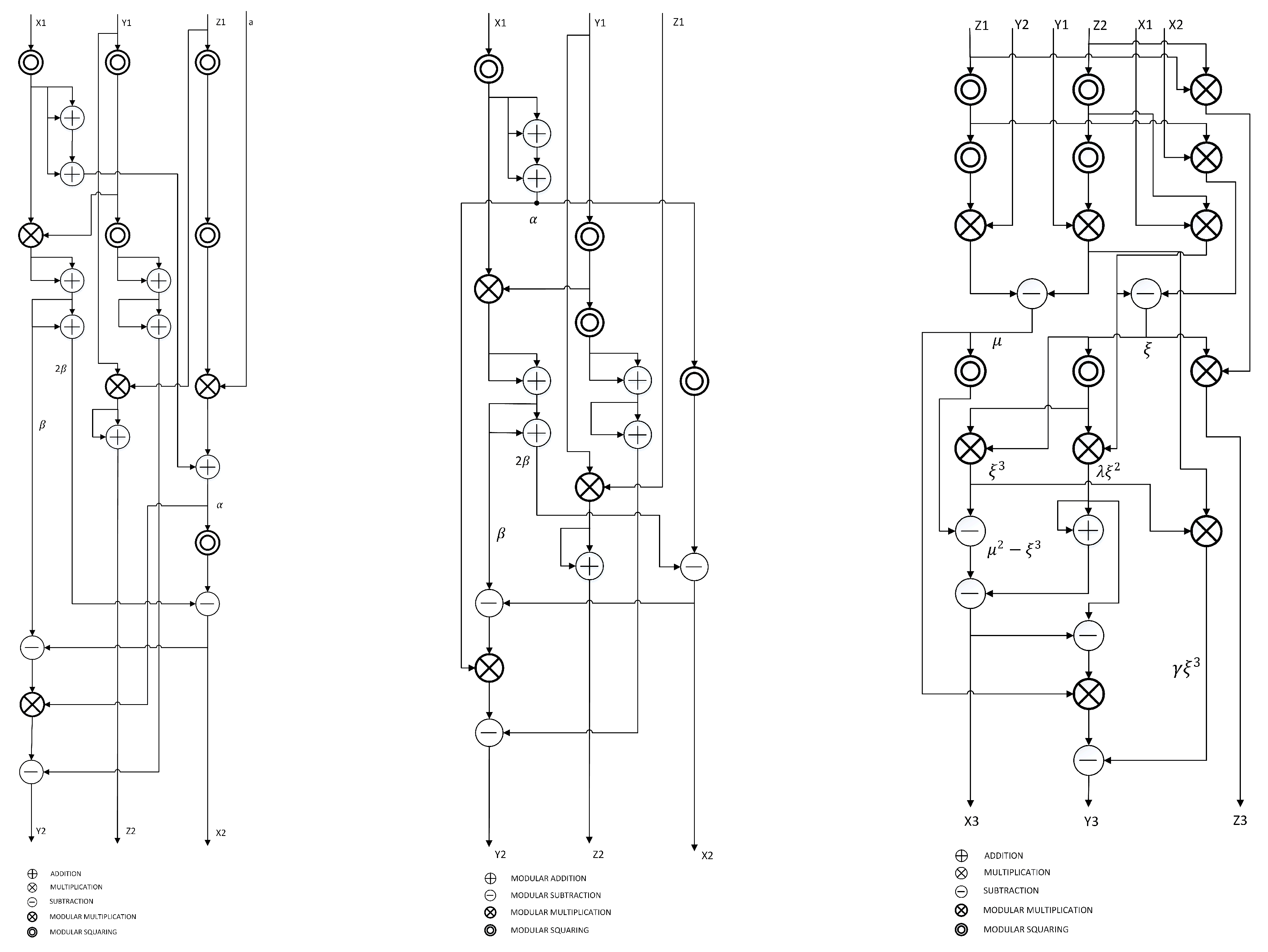
3.3. Point Doubling in Jacobian Coordinates

This section gives the formulas used for implementing point doubling.

Suppose: P$(X_1,Y_1,Z_1)$ and

$$\alpha =3X_1^2+\alpha Z_1^4,\beta =4X_1{Y}_1^2,$$

(2)

Point Q on curve E is defined as: $Q(X_2,Y_2,Z_2)=2.P(X_1,Y_1,Z_1)$

$$X_2={\alpha }^2-2\beta ,$$

(3)

$$Y_2=\alpha (\beta -X_2)-8Y_1^4,$$

(4)

$$Z_2=2Y_1{Z}_1,$$

(5)

3.4. Point Addition in Jacobian Coordinates

This section gives the formulas used for implementing point addition. Suppose: $P_1(X_1,Y_1,Z_1)$ and $P_2(X_2,Y_2,Z_2)$ are two points on curve (E) and

$$\gamma =Y_1{Z}_2^3,\lambda =X_1{Z}_2^2,\mu =Y_2{Z}_1^3-Y_1{Z}_2^3,\xi =X_2{Z}_1^2-X_1{Z}_2^2,$$

(6)

The new point P3 on Curve (E) such that: $P_3(X_3,Y_3,Z_3)$ = $P_1(X_1,Y_1,Z_1)$ + $P_2(X_2,Y_2,Z_2)$ is:

$$X_3={\mu }^2-{\xi }^3-2\lambda {\xi }^2$$

(7)

$$Y_3=\mu (\lambda {\xi }^2-X_3)-\gamma {\xi }^3,$$

(8)

$$Z_3=Z_1{Z}_2\xi ,$$

(9)

All calculations are to be done in finite field $F_p$, meaning that mod p reduction is applied to Formulas (2)–(9).

A modular reduction unit is designed based on an interleaved modular multiplier architecture similar to the one proposed in [33,34]. Based on the implementation results in [33,34], an interleaved modular multiplier has more efficient area and timing characteristics. For fast and area-efficient implementation of such a multiplier, we use just one CSA adder and a look-up table. The structure of our design is depicted in Figure 1.

The look-up table code is given by;

LUT(0) = 0;
LUT(1) = Y;
LUT(2) = 2 ∗ 2ⁿ mod M;
LUT(3) = (2 ∗ 2ⁿ + Y) mod M;
LUT(4) = 4 ∗ 2ⁿ mod M;
LUT(5) = (Y + 4 ∗ 2ⁿ) mod M;
LUT(6) = 6 ∗ 2ⁿ mod M;
LUT(7) = (Y + 7 ∗ 2ⁿ) mod M;
and
(S,C) = CSA(A,B,C) is

$$S_i=A_i⨁B_i⨁C_i,$$

$$C_{i+1}=(A_i.B_i)V(A_i.C_i)V(B_i.C_i),C_0=0$$

The modular multipliers use one clock cycle to register inputs, 256 (n) clock cycles in the loop, one clock cycle to calculate the CSA addition and one clock to register output, so the calculation is done in just 259 n + 3 clock cycles.

3.5. ECC Core Design

The ECC core design gets a point on the ECC curve in Jacobian coordinates P(X,Y,Z) and calculates point Q = kxP within the same coordinate system. Figure 1 illustrates the ECC core design.

3.6. Elliptic-Curve Point Doubling—ECPD

Point doubling uses three modular multiplier units to calculate (2)–(5) in parallel. Ten modular multiplications are done in five stages that reduce the point-doubling calculation time to 5(n + 3) + 4 clock cycles.

For curve SECP256K1, as a = 0, the logic can be reduced. Using just one modular reduction unit, ECPD can be performed at 7 logic levels or 7(n + 3) + 2 clock cycles by the optimized-area ECPD. Figure 2 shows the data-flow diagram of the ECPD doubling with and without optimized area.

3.7. Elliptic-Curve Point Addition

Point addition uses three modular multiplier units to calculate point Q + P on the elliptic curve in parallel. Sixteen modular multiplications are done in seven stages as shown in Figure 2, so the latency of point addition will reduce to 7(n + 3) + 5 clock cycles.

3.8. Scalar Factor (Private Key) k

The scalar factor ’k’ is stored in internal RAM and can be changed via software command. To implement a point multiplication, the double-and-add-always algorithm is used as given in Algorithm 1. A point doubling is done followed by a point addition at every stage i, but the result of the point addition is used only when the ith bit of the scalar k is ’1’. Otherwise, the result of point addition will not be used.

In this method, N times PD and PA are required (here N = 256). This algorithm uses the same hardware resources for the zero and one bits of the key k, so the power consumption during calculations is homogeneous. The resources consumed by the design of the interleaved multiplier are given in

Table 1. Implementation results on Xilinx FPGA XC7k160tfbg676-1.

Resource	Utilization
CORE AREA (LUT)	26,570
ECPA (LUT)	14,382
ECPD (LUT)	11,760
CLK frequency	100.00 MHz
DYNAMIC POWER	0.20 W
TOTAL POWER	0.313 W

.

4. Attack Methodology

The purpose of this research is to capture and analyze the power-consumed signals of the FPGA (Kintex-7) while the ECC double-and-add-always algorithm is encrypting data with a secret key. The idea is to attack one bit at a time. For our analysis, we will attack the least-significant three bits of the nibble i.e., bit 2, bit 3 and bit 4. The bit at location one does not need to be attacked as it does not contribute to the encryption. To achieve this purpose, a random 31-bytes (which are the most significant 248 bits) fixed key is selected and the value of the last byte is changed in ascending order, from $2^1$ till $2^4-1$. For further simplification, in this paper we have attacked bit locations 2, 3 and 4 only, and bit locations 5 to 8 are set to “0000“. From now on, ’key’ refers to the last nibble of the key as shown in Figure 3.

For the analysis, machine-learning classification will be used. For classification using machine learning, the data samples should consist of the properly labeled features. We propose to use a different set of features as opposed to the raw samples’ amplitude, which leads to a division of our attack into two main steps:

• Step 1—Training dataset preparation
• Step 2—Classification using machine learning

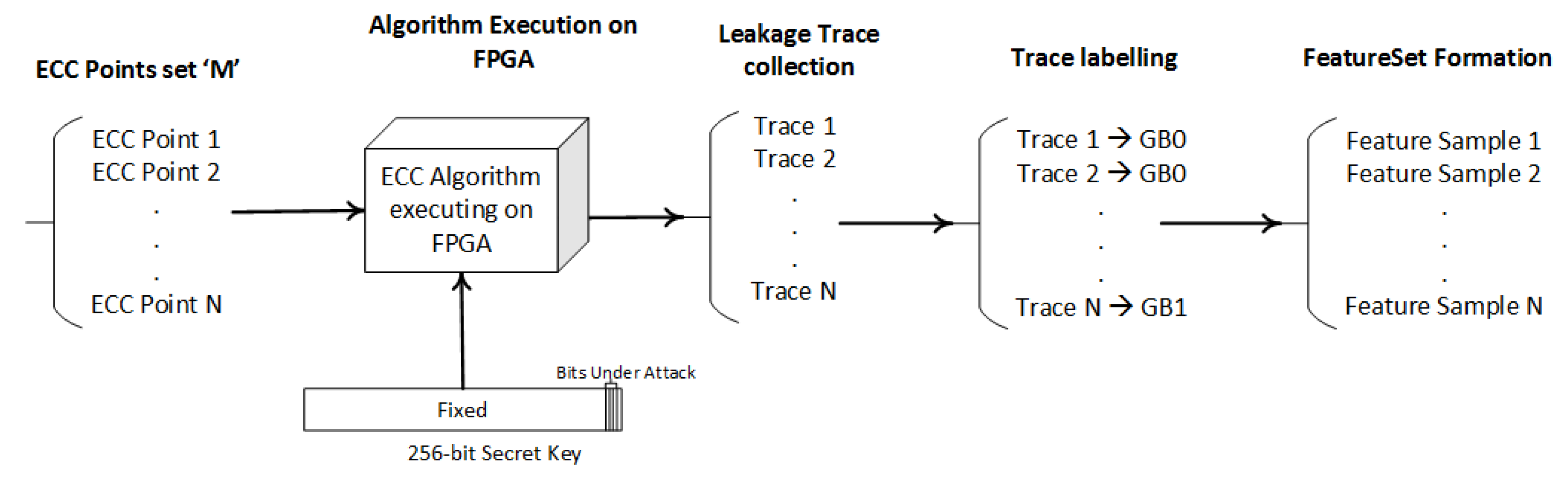
4.1. Step 1—Training Dataset Preparation

Let N be the number of randomly selected ECC points, in the Jacobian coordinate system, from the elliptic curve E, and M represent the set of ECC points, then each ECC point in M, over curve E, can be represented as follows:

$$M=\{(X_i,Y_i,Z_i)\mathrm{where}i=1,2,\dots N\}$$

(10)

Let K be the least-significant four bits of the 256-bit key. Out of the 4 LSBs, the three bits at locations 2nd, 3rd and 4th, are the target of this analysis. The first bit is not considered, as the double-and-add-always algorithm’s implementation starts encryption using a second bit of the key. For each bit location, raw traces of length $Le{n}_{Trace}$ are collected and then processed to form samples. $S_{BitLoc}=N\ast S_{p}t$ samples are collected for N ECC points from the set M, where $S_{p}t$ represents the number of samples for each ECC point from the pool of N ECC points. As the number of possible combinations for the last nibble is $2^4$ and there is no point in attacking the first bit, so in total $S_N=S_{BitLoc}\ast (2^n-2)$ samples are collected. For creating a training dataset for machine-learning classification, data samples need to be labeled. After data sample collection, labeling is an important task. To ease the process of attacking and labeling, we have divided the attack into three levels according to the bit location under attack and have categorized the samples into two groups. Each is further explained below.

4.1.1. Group Labeling

All data samples are divided into two groups ’GB0’ and ’GB1’. GB0 means that the sample represents a bit ’0’ and GB1 means that the sample represents a bit ’1’. Each attack level will have different samples marked as GB0 or GB1 according to the bit location.

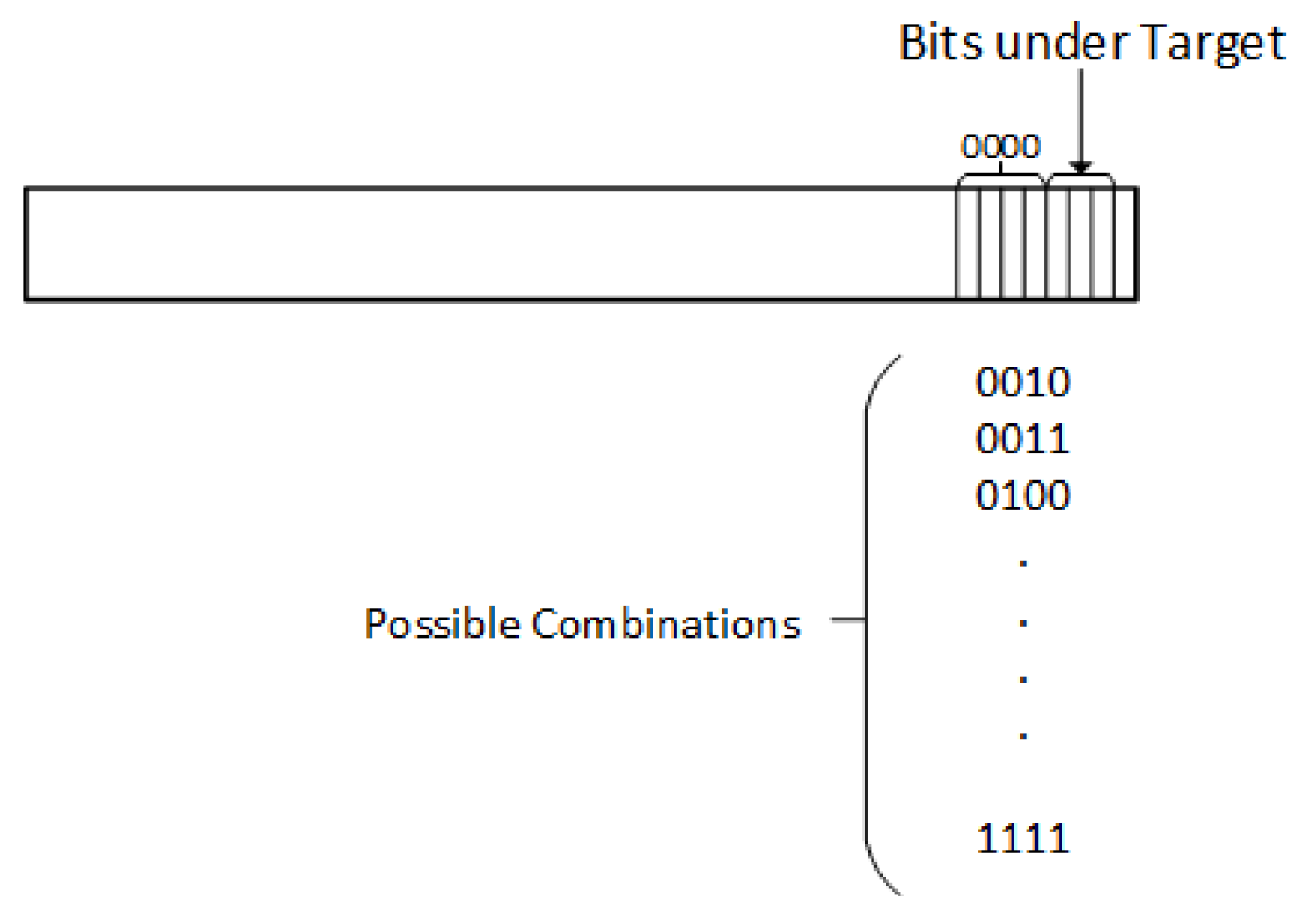
4.1.2. Attack Levels

Attack levels are designed based on the bit locations under attack, called ’LB{b}’. LB stands for the ’Location bit’ and ’b’ represents the actual location of the bit. Based on this information, three bit levels are defined as follows.

• LB2—At this attack level, LSB ’2’ is targeted and each sample for the key having ’0’ at the second location is marked as ’GB0’ and all samples for the key byte having ’1’ at the second location are marked as ’GB1’.
• LB3—At this attack level, LSB ’3’ is targeted and each sample for the key having ’0’ at the third location is marked as ’GB0’ and all samples for the key byte having ’1’ at the third location are marked as ’GB1’.
• LB4—At this attack level, LSB ’4’ is targeted and each sample for the key having ’0’ at the fourth location is marked as ’GB0’ and all samples for the key byte having ’1’ at the fourth location are marked as ’GB1’.

The attack levels along with the labeling of the samples are shown in Figure 4.

4.1.3. Features Dataset Formation

As all the raw samples have been labeled, the next step is to calculate the features. For our analysis, we have used time-domain and frequency-domain signal properties as features. The reason for selecting these particular signal properties is based on our previous analysis on AES leaked data. We selected and analyzed more than six signal properties and concluded that a combination of time-domain and frequency-domain signal properties leads to better classification [26,29]. An explanation of each signal property (used in this work) is given below:

• Mean of Absolute Value (MAV)—Mean of the signal is calculated.
• Kurtosis (Kur)—For Kurtosis, Frequency-distribution curve peak’s sharpness is noted.
• Median PSD (FMD)—For Median PST, median is calculated in frequency domain.
• Frequency Ratio (FR)—For Frequency ratio, frequency ratio of the frequencies is recorded.
• Median Amplitude Spectrum (MFMD)—For MFMD, the median amplitude spectrum of signals is calculated.

For all the captured $S_N$ samples, the above-mentioned features are calculated, returning one sample value for each instead of $Le{n}_{Trace}$, hence reducing the data sample size, which is the advantage of using the above-proposed features.

The overall training dataset preparation process is shown in Figure 5.

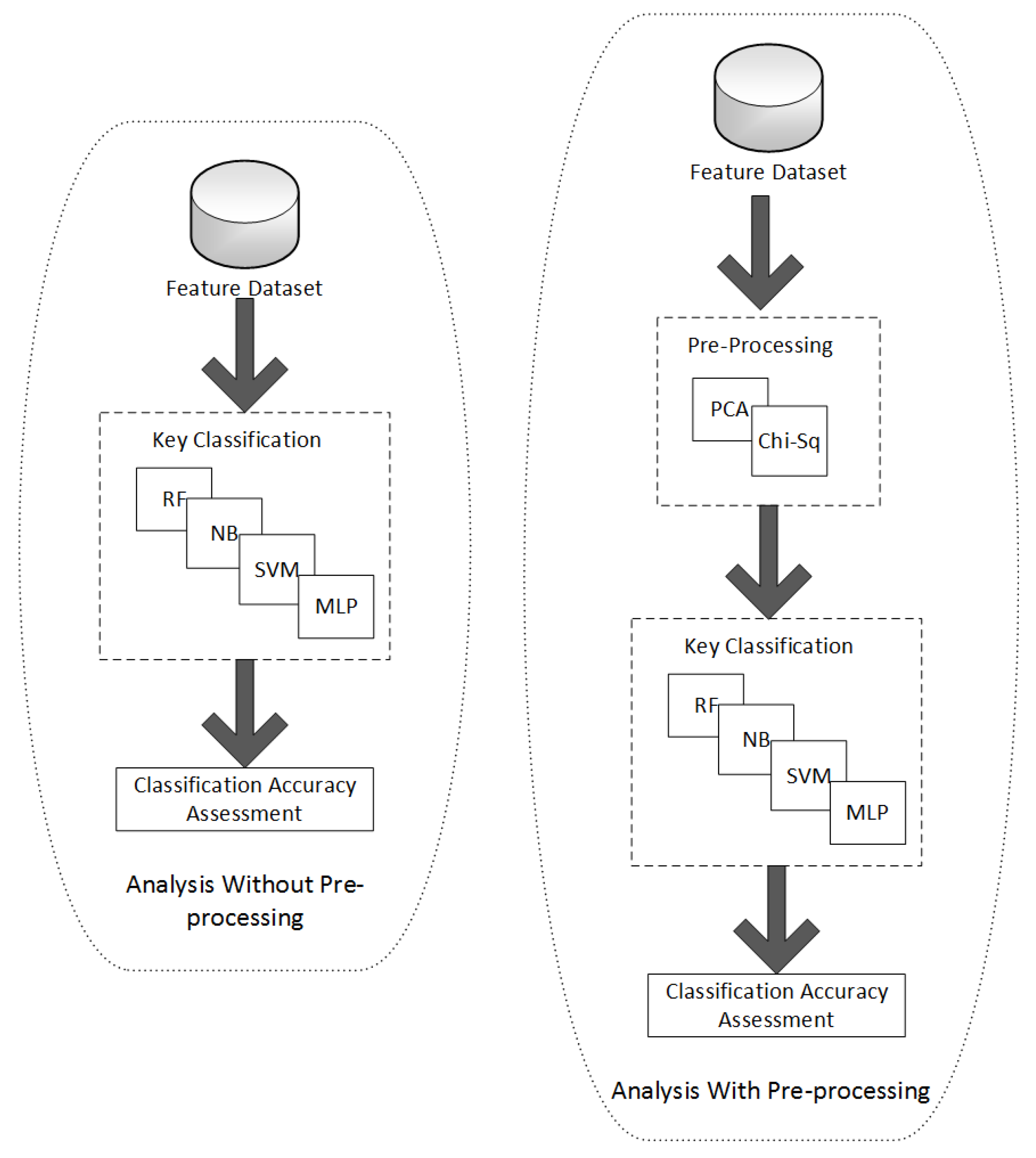
4.2. Step 2—Classification Using Machine Learning

Traditionally, statistical methods are used to perform the analysis but for this research machine-learning and neural-network-based classifiers are applied on the feature datasets, formed in Section 4.1. The classification algorithms selected for analysis are Support Vector Machines (SVM), Naive Bayes (NB), Random Forest (RF) and Multilayer Perceptron (MLP). An explanation of each is given in Section 2.2. According to author’s knowledge, there is very little work done in the field of machine-learning-based power analysis on elliptic curves which includes analysis of ECC leaked data (from a FPGA) using PCA-SVM. Hence, in our analysis, the comparison is provided with respect to the machine-learning-based analysis only.

There are two parts of the analysis as given below.

4.2.1. Analysis without Pre-Processing

In the first phase of analysis, classification is performed on the feature datasets without any pre-processing. This analysis will help in identifying the impact of using signal properties as features.

4.2.2. Analysis with Pre-Processing

In the second phase of analysis, the feature dataset is first processed through a feature selection and extraction mechanism before training the model and is then subjected to the classification. The feature selection and extraction techniques used for pre-processing are PCA and Chi-Square (Chi-Sq). Details are given in Section 2.4. The signals’ noise makes the side-channel attacks harder to launch. The evaluators/selectors are used to filter out the features to overcome the problem of noisy signals, hence reducing the training time and computational complexity. Another benefit of using these extractors/selectors is to reduce the possibility of a wrong classification. For testing the trained model, another feature dataset is formed based on the same methodology. This is done to gain more confidence in the results, as it ensures that the model has never seen the test data before. The process of classification on the training feature dataset is shown in Figure 6. Moreover, the effect of changing of various variables/parameters was observed. The time required to build the model has also been recorded.

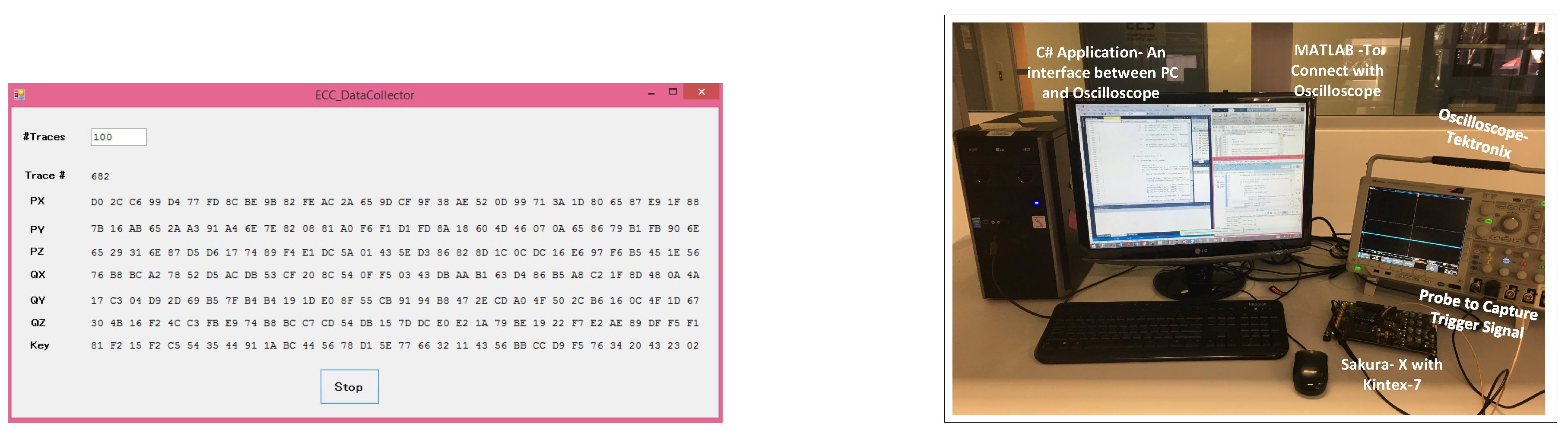
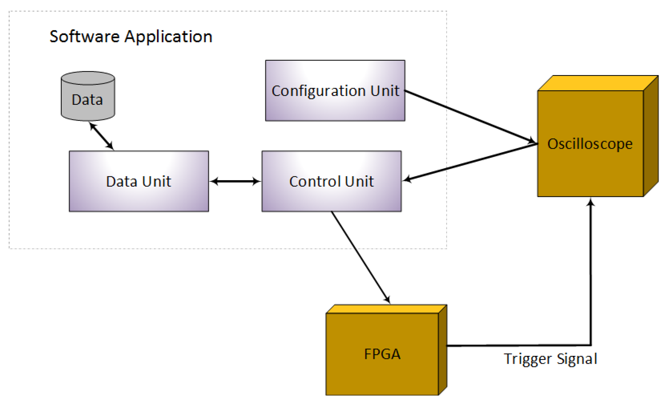
5. Experimental Setup

This section explains the hardware and software setup for testing the methodology explained in the above sections.

5.1. Step 1—Data Capture

To conduct our experiments, we must capture the leakage traces, as a power signals database for ECC does not exist. For the hardware setup, we captured the power signals for ECC FPGA (Kintex-7) implementation, operating at 24 MHz. For this research, specialized side-channel analysis board, named as SAKURA-X, is used [35]. On SAKURA-X, for calculating the power being consumed, a resistor is connected in series and a voltage is measured across that. The user does not need to tweak the board, as the connector is available to get the power signal directly. Traces are captured using a Tektronix oscilloscope having a 5 $GS/sec$ sampling frequency and a 1 GHz bandwidth. We have acquired N = 100 traces for randomly selected ECC points from set M, and for each point $S_{p}t$ = 10 traces were captured. Thus, in total $S_N$ = 14,000 traces are collected where each trace has 10 k sampling points.

For the software side of the data-collection process, we have developed bespoke codes using C# and the MATLAB library to form an automated standalone application which requires little or no intervention from the user. The hardware setup and the application GUI is shown in Figure 7. A few modules of the C# application provided by SAKURA are used to achieve the purpose [35]. The new bespoke C# application consists of three main units: control unit, data unit, and configuration unit as shown in Figure 8, and an explanation of each is given below.

• Configuration Unit—The configuration unit uses MATLAB library support for C# and configures the oscilloscope through the C# application. This eliminates setting up the oscilloscope on every start up; the application automatically restores it to the settings required for the data capturing. The configuration unit communicates with the oscilloscope only.
• Control Unit—The control unit has the role of sending the ECC points to the FPGA after taking them from the data unit. When the FPGA receives an ECC point, it starts the process of encryption and sends a trigger signal to the oscilloscope. As soon as the trigger signal is received at the oscilloscope, it will start collecting the leaked information from the FPGA and will transmit it to the control unit. The control unit then stores the information by communicating with the data unit. The control unit communicates with both the oscilloscope and the FPGA.
• Data Unit—The data unit handles the data. It is responsible for storing and retrieving the data in files. The data unit communicates with the control unit only.

5.2. Step 2—Feature Datasets Formation

After collection of the raw traces, samples are labeled according to the description given in Section 4.1.1, using a bespoke java snippet. After labeling, features (properties) are calculated using bespoke MATLAB code, and act as features for further classification.

5.3. Step 3—Analysis

Classification models are then trained, using the proposed feature datasets. Feature datasets are trained and tested with and without applying the pre-processing filters. For training and testing, tools like weka and organe3 are used [36]. Parameters settings for each classification algorithm are discussed in the results.

6. Results and Discussion

Results and discussion are divided into four sections. In each section, results are discussed with reference to classification algorithms.

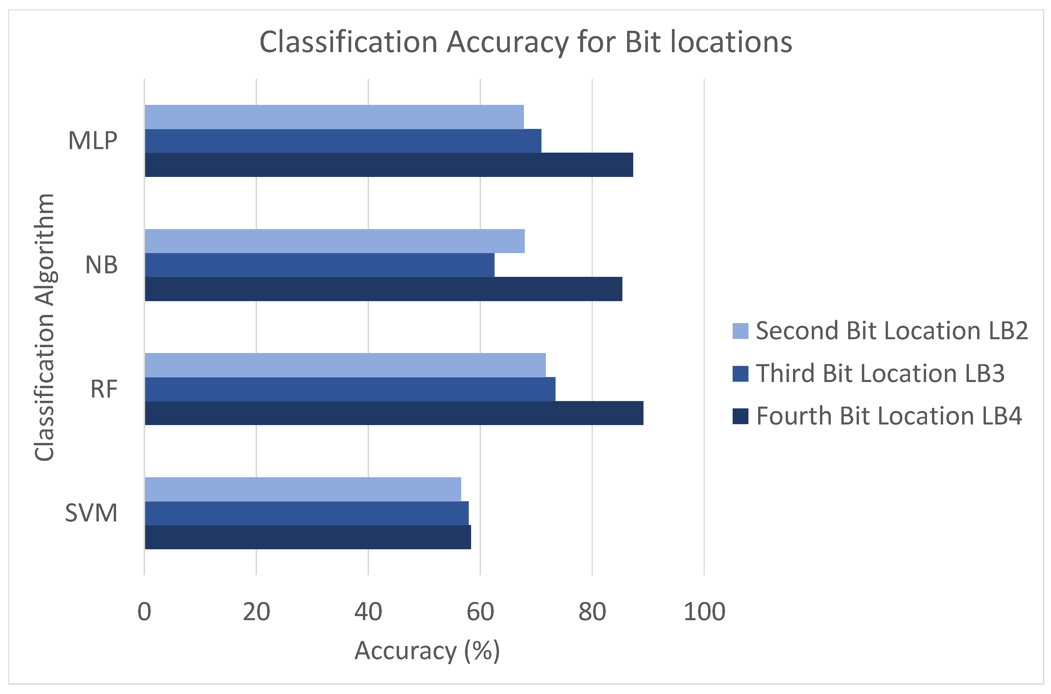
6.1. Analysis Phase 1—Accuracy without Pre-Processing

In the first part of phase-1 analysis, the classification accuracy is calculated on the raw-signal feature data set. It is observed that RF gives an accuracy of 79% for LB4. For NB, SVM and MLP, the accuracy is even lower i.e., 52%, 55% and 71%. For LB2 and LB3, the accuracy is less than LB4, as shown in

Table 2. Accuracy for Raw sample analysis.

Algorithm	LB4	LB3	LB2
RF	79.2%	56.9%	58.0%
SVM	55.4%	49.3%	45.7%
MLP	71.9%	58.7%	55.6%
NB	52.5%s	57.0%	55.7%

. These results clearly show that the data cannot be correctly classified due to the large number of features in the dataset.

In the second part of phase-1 analysis, the classification accuracy is calculated on the proposed processed feature datasets without any pre-processing (i.e., feature selector/extractor) for all three levels of attack (LB2-LB4), as given in Figure 9. Models are trained and tested using the four classifiers SVM, RF, NB, and MLP. It can be seen that, without the pre-processing step, SVM does not perform well for any level of bit classification. However, for the fourth-bit classification, RF gives an accuracy of approximately 90% while NB and MLP give an accuracy of 85% and 88%, respectively. RF and NB perform well for the datasets in which the features are completely independent of each other. These results prove that the features in the signals feature datasets (for fourth-bit location) are independent of each other.

For bit 2 and bit 3 classification, the maximum accuracy achieved is 71–73% with RF. Both SVM and MLP perform poorly in these cases. The reason for MLP’s low performance could be the feature dataset size. For neural-network algorithms, the training data should be huge, roughly a hundred times more than the number of features in each trace/row. It is worth exploring if MLP or any other neural network can behave better if the number of samples is increased for better training. This analysis is out of the scope of this paper and is a future prospect of this particular research.

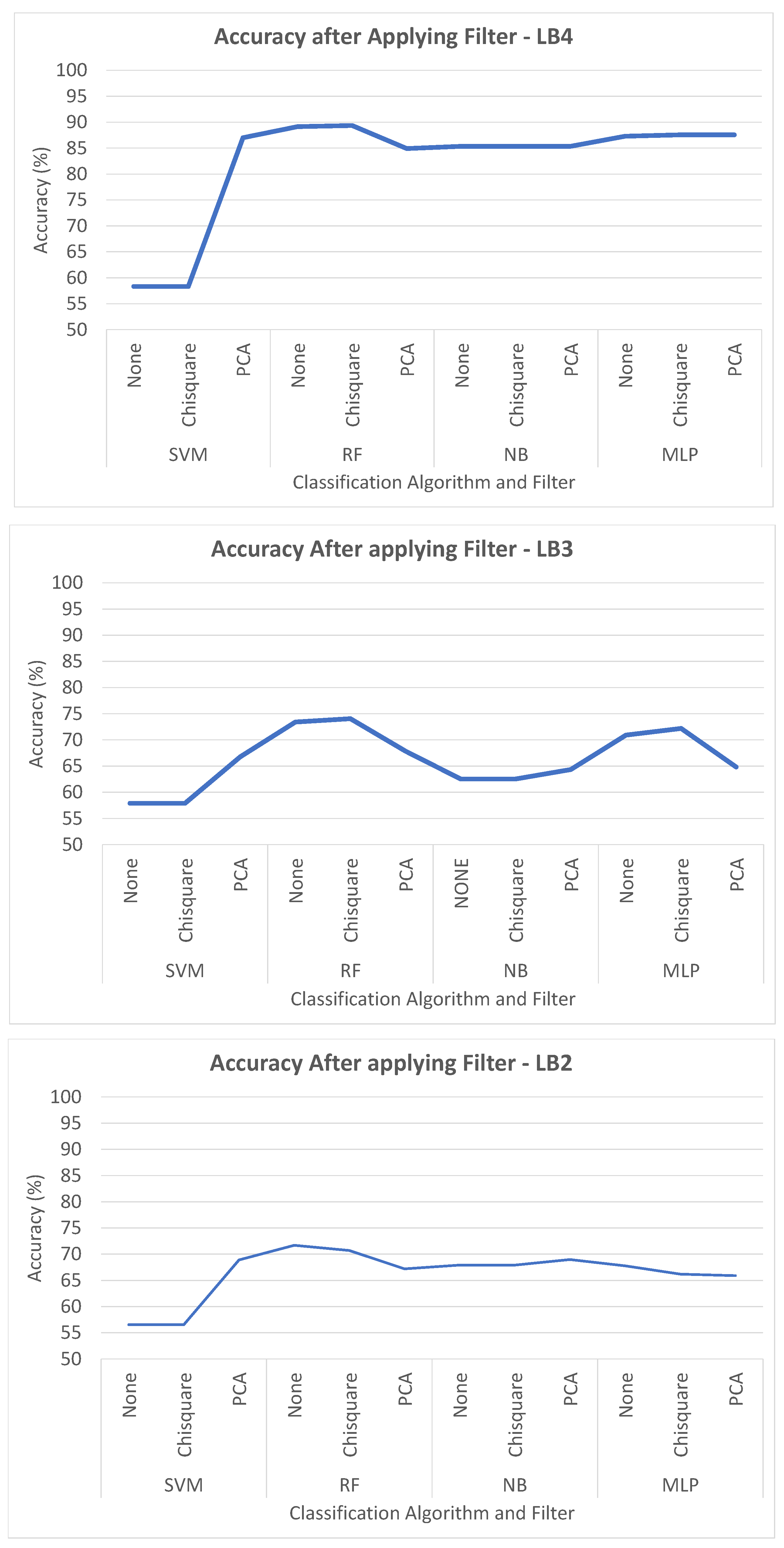
6.2. Analysis Phase 2—Accuracy with Pre-Processing

In the second phase of the analysis, the classification accuracy is calculated on the feature datasets after pre-processing them using the feature selectors/extractors. The results of ’LB2’, ’LB3’ and ’LB4’ are given in Figure 10. The results show that if PCA is applied then, for SVM, the accuracy improves for all three cases. This happens because the obtained traces are noisy, having redundant information. PCA extracts the important features/components so when SVM is applied on the reduced feature set then the accuracy is improved. The maximum accuracy attained is 87% for ’LB4’. However, Chi-square did not show any improvement in any of the LBs. It is worth noting that the accuracy of RF got worst after pre-processing with PCA, because RF works on the assumption that there is no dependence between features. PCA reduces the number of features and at the same time removes the col-linear features from the feature dataset. For MLP, accuracy increases after applying filters in case of LB4 but strange behavior is observed in case of LB3 and LB2, which requires further analysis.

The authors in [37] have obtained 96% accuracy after applying SVM on 4-bit implementation of ECC leaked data. Our results of classification algorithms are obtained after applying SVM on 256-bit key (out of which first 31 bytes of the key are fixed random numbers). Our results show that, with PCA-SVM, accuracy of around 86% can be achieved to recover the least-significant nibble from a 256-bit key.

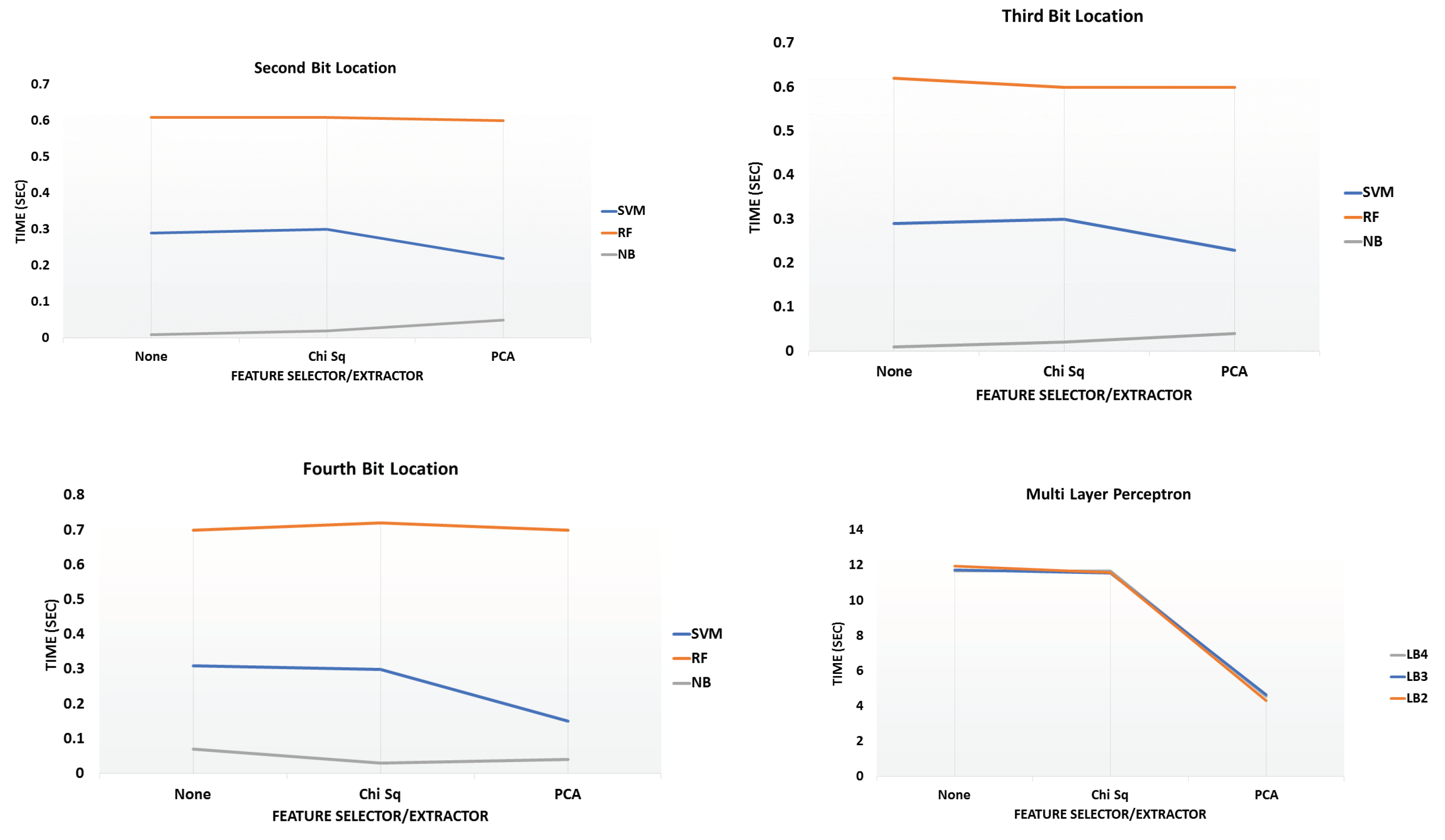
6.3. Analysis Phase 3—Time to Build Models

It has been seen that the time taken to build the model with raw signals varies from 90–150 s for classifiers. However, the time taken to build the model on the proposed processed feature dataset is less. The reason is obviously that, with raw signals, the number of features per trace is 10 k times more than for the proposed processed feature datasets. In particular it was observed that the time taken to build the model for the MLP, with proposed processed feature dataset, is more than the time taken by SVM, RF and NB. After applying PCA, the time taken to build the model is reduced in all cases (LB2–LB4) for all algorithms, as can be seen from Figure 11. The reason for the decrease in the time required to build the model is that the number of features is reduced after applying filters.

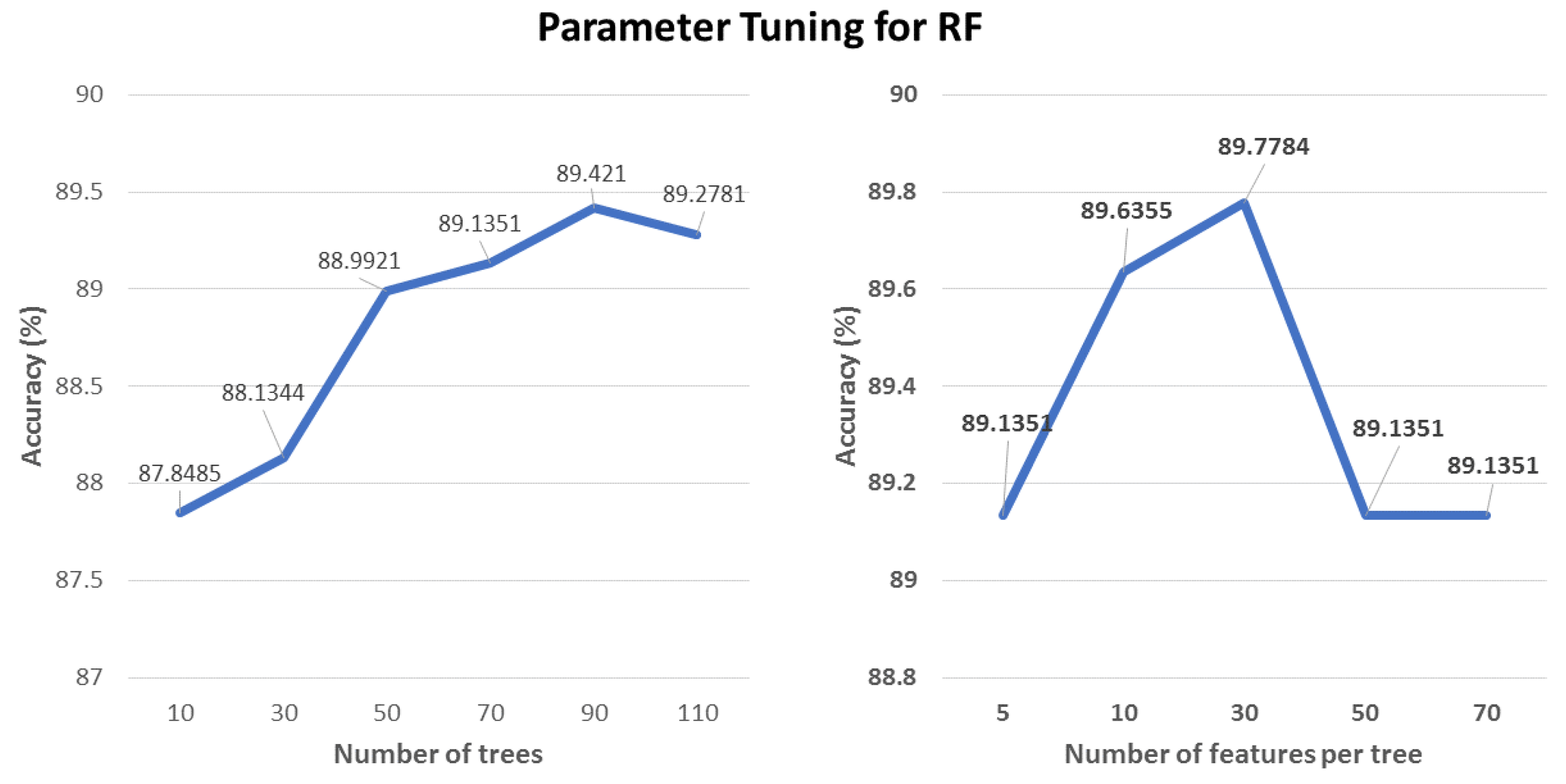
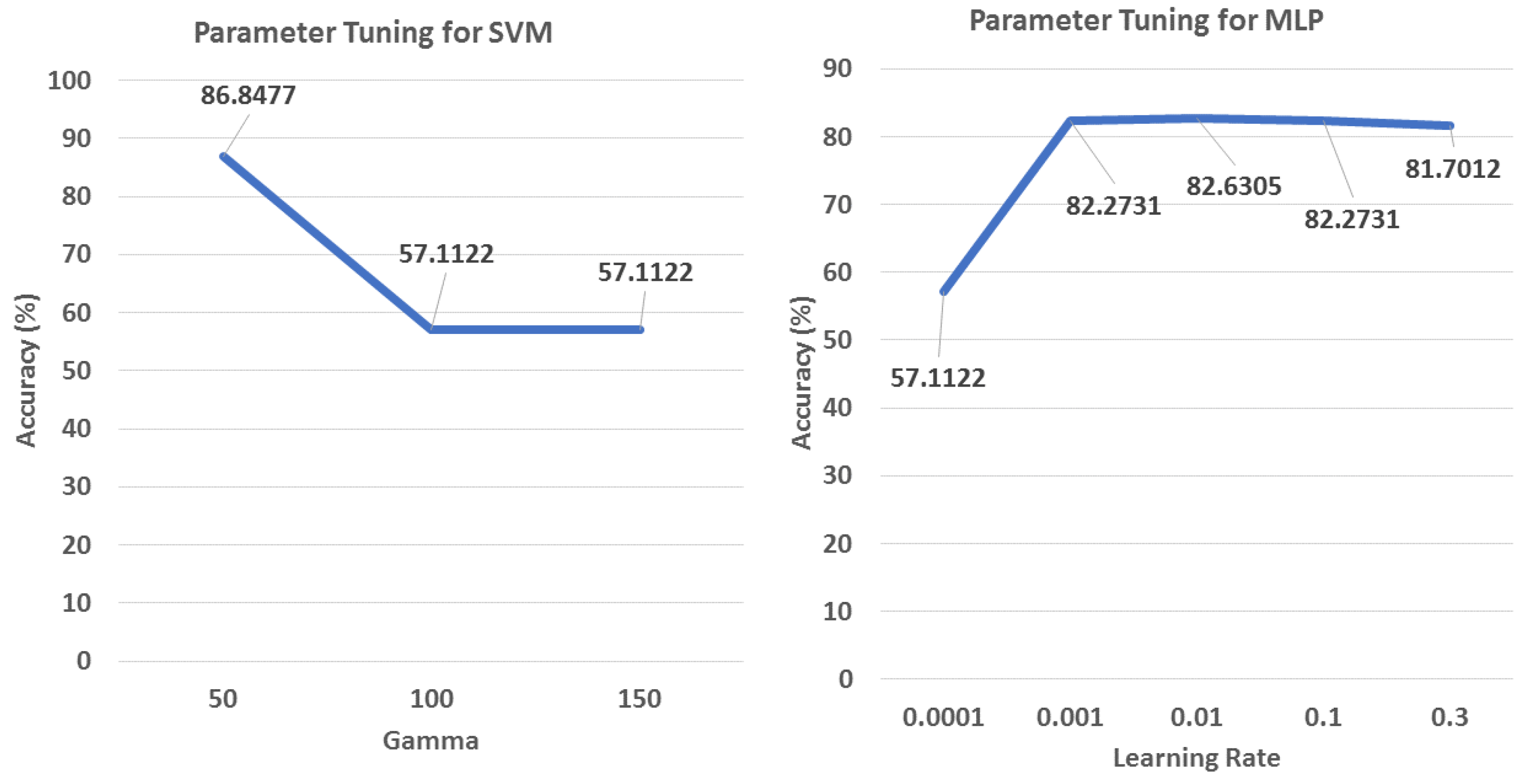
6.4. Hyper-Parameter Tuning

Based on the analysis so far, the best-performing combination of filters and classifier is selected, and different parameters are tuned for LB4. The parameters used for analysis, using four classification algorithms, are discussed below.

The parameters tuned for RF are the number of trees and the number of features per tree. Experimental results show that with 90 trees within the forest, the highest accuracy of approximately 89.4%, is achieved. The accuracy decreases if the number of trees is increased or decreased beyond 90. Therefore, 90 trees are selected for further analysis, and number of features per tree are changed, when it is observed that maximum accuracy is obtained when the number of features per tree is 30, as shown in Figure 12.

In NB, two important parameters are kernel estimator and supervised discretization. It was observed that turning on kernel estimator gives an accuracy of 86.77%. However, accuracy is increased if supervised discretization mode is turned on.

For SVM, gamma is changed to see the effect on accuracy. As SVM uses nonlinear kernel functions, so a lower gamma value means low bias and high variance. It is seen that with higher values of gamma, the accuracy decreases as can be seen from Figure 13.

For any neural network, the two most important parameters to analyze are the change of learning rate and the batch size. For this analysis, the number of neurons is fixed, and one hidden layer is used. Learning rate is the rate of training with which the model is trained, and the batch size is the number of samples that are given to the model for one training period. It was observed that the batch size does not have any effect on the accuracy. However, the model is trained best with learning rate of 0.01, as can be seen from Figure 13.

7. Conclusions

After analyzing the results on the power-consumed signals obtained from the Kintex-7, we can conclude that signal properties of the captured leaked power signals can be used as features, as they give an accuracy of approx. 90% with RF. This means that we can recover the secret key from the leaked signals with approx. 90% accuracy. For classification algorithms like RF, NB, and MLP, pre-processing did not show any improvement at all, because these classifiers already perform well for noisy data having redundant information. However, for SVM, using PCA as a pre-processing step improved the accuracy to 86%, as PCA extracted the important relevant features. SVM still shows less accuracy than the others. Moreover, the time taken for building the model has been analyzed and it is observed that the time for training the model is more for raw signals and for the neural-network-based MLP model. The parameters for all four classification algorithms have been tuned and the best recommendations are put forward in the paper.

8. Future Work

Future work will be based on the findings of this research. We aim to recover the middle and initial most significant bits of the key. As RF performs the best, the first preference for all future analysis would be RF. As the data samples would be different for the key bits according to their locations, which might introduce non-linearity in the system, thus increasing the possibility of improved attack accuracy using neural networks. We would like to analyze the data using deep-learning algorithms like Convolutional Neural Networks and Long-Short-Term-Memory networks, to explore these avenues.

References

1. Kocher, P.C. Timing Attacks on Implementations of Diffie-Hellman, RSA, DSS, and Other Systems. In Proceedings of the Advances in Cryptology—CRYPTO ’96: 16th Annual International Cryptology Conference, Santa Barbara, CA, USA, 18–22 August 1996; Springer: Berlin/Heidelberg, Germany, 1996; pp. 104–113. [Google Scholar]
2. Kocher, P.C.; Jaffe, J.; Jun, B. Differential Power Analysis. In Proceedings of the Advances in Cryptology—CRYPTO’ 99: 19th Annual International Cryptology Conference, Santa Barbara, CA, USA, 15–19 August 1999; Springer: Berlin/Heidelberg, Germany, 1999; pp. 388–397. [Google Scholar]
3. Rivest, R.L. Cryptography and machine-learning. In Proceedings of the Advances in Cryptology—ASIACRYPT ’91: International Conference on the Theory and Application of Cryptology, Fuji Yoshida, Japan, 11–14 November 1991; Springer: Berlin/Heidelberg, Germany, 1993; pp. 427–439. [Google Scholar]
4. Genkin, D.; Pachmanov, L.; Pipman, I.; Tromer, E.; Yarom, Y. ECDSA Key Extraction from Mobile Devices via Nonintrusive Physical Side Channels. In Proceedings of the 2016 ACM SIGSAC Conference on Computer and Communications Security, Vienna, Austria, 2016; ACM: New York, NY, USA; pp. 1626–1638. [Google Scholar]
5. Kadir, S.A.; Sasongko, A.; Zulkifli, M. Simple power analysis attack against elliptic curve cryptography processor on FPGA implementation. In Proceedings of the 2011 International Conference on Electrical Engineering and Informatics, Bandung, Indonesia, 17–19 July 2011; pp. 1–4. [Google Scholar]
6. Genkin, D.; Shamir, A.; Tromer, E. RSA Key Extraction via Low-Bandwidth Acoustic Cryptanalysis. In Proceedings of the Advances in Cryptology—CRYPTO 2014: 34th Annual Cryptology Conference, Santa Barbara, CA, USA, 17–21 August 2014; pp. 444–461. [Google Scholar]
7. Standaert, F.X.; tot Oldenzeel, L.V.O.; Samyde, D.; Quisquater, J.J. Power Analysis of FPGAs: How Practical Is the Attack? In Proceedings of the Field Programmable Logic and Application, Lisbon, Portugal, 1–3 September 2003; Springer: Berlin/Heidelberg, Germany, 2003; pp. 701–710. [Google Scholar]
8. Yalcin Ors, S.B.; Oswald, E.; Preneel, B. Power-Analysis Attacks on an FPGA—First Experimental Results. In Proceedings of the Cryptographic Hardware and Embedded Systems (CHES), Cologne, Germany, 8–10 September 2003; Springer: Berlin/Heidelberg, Germany, 2003; pp. 35–50. [Google Scholar]
9. De Mulder, E.; Ors, S.B.; Preneel, B.; Verbauwhede, I. Differential Electromagnetic Attack on an FPGA Implementation of Elliptic Curve Cryptosystems. In Proceedings of the Automation Congres, Budapest, Hungary, 24–26 July 2006; pp. 1–6. [Google Scholar]
10. Longo, J.; De Mulder, E.; Page, D.; Tunstall, M. SoC it to EM: Electromagnetic Side-Channel Attacks on a Complex System-on-Chip; Cryptographic Hardware and Embedded Systems—CHES; Lecture Notes in Computer Science; Springer: Berlin, Germany, 2015; Volume 9293, pp. 620–640. [Google Scholar]
11. Gierlichs, B.; Batina, L.; Tuyls, P.; Preneel, B. Mutual information analysis. In Proceedings of the Cryptographic Hardware and Embedded Systems—CHES, Washington, DC, USA, 10–13 August 2008. [Google Scholar]
12. Renauld, M.; Standaert, F.; Veyrat-Charvillon, N. Algebraic Side-Channel Attacks on the AES: Why Time also Matters in DPA. In Proceedings of the Cryptographic Hardware and Embedded Systems—CHES 2009, Lausanne, Switzerland, 6–9 September 2009; Springer: Berlin/Heidelberg, Germany, 2009; pp. 97–111. [Google Scholar]
13. Bhasin, S.; Danger, J.; Guilley, S.; Najm, Z. Side-Channel Leakage and Trace Compression using Normalized Inter-Class Variance. In Proceedings of the 3rd International Workshop on Hardware and Architectural Support for Security and Privacy, HASP, Portland, OR, USA, 14 June 2015; p. 7. [Google Scholar]
14. Oswald, D.; Paar, C. Improving Side-Channel Analysis with Optimal Linear Transforms. In Proceedings of the 11th International Conference on Smart Card Research, and Advanced Applications, CARDIS, Graz, Austria, 28–30 November 2012; Springer: Berlin/Heidelberg, Germany, 2013; pp. 219–233. [Google Scholar]
15. Hospodar, G.; Mulder, E.D.; Gierlichs, B.; Verbauwhede, I.; Vandewalle, J. Least Squares Support Vector Machines for Side-Channel Analysis. In Proceedings of the 2nd Workshop on Constructive Side-Channel Analysis and Secure Design (COSADE), Darmstadt, Germany, 24–25 February 2011. [Google Scholar]
16. Willi, R.; Curiger, A.; Zbinden, P. On Power-Analysis Resistant Hardware Implementations of ECC-Based Cryptosystems. In Proceedings of the 2016 Euromicro Conference on Digital System Design (DSD), Limassol, Cyprus, 31 August–2 September 2016; pp. 665–669. [Google Scholar] [CrossRef]
17. Batina, L.; Hogenboom, J.; van Woudenberg, J.G.J. Getting More from PCA: First Results of Using Principal Component Analysis for Extensive Power Analysis. In Proceedings of the Cryptographers? Track at the RSA Conference, San Francisco, CA, USA, 27 February–2 March 2012; Springer: Berlin/Heidelberg, Germany, 2012; pp. 383–397. [Google Scholar]
18. Souissi, Y.; Nassar, M.; Guilley, S.; Danger, J.L.; Flament, F. First Principal Components Analysis: A New Side Channel Distinguisher. In Proceedings of the International Conference on Information Security and Cryptology, Seoul, Korea, 1–3 December 2010; pp. 407–419. [Google Scholar] [CrossRef]
19. Lerman, L.; Bontempi, G.; Markowitch, O. A machine learning approach against a masked AES. J. Cryptogr. Eng. 2013, 5, 123–139. [Google Scholar] [CrossRef]
20. Lerman, L.; Bontempi, G.; Markowitch, O. Power analysis attack: An approach based on machine learning. Int. J. Appl. Cryptogr. (IJACT) 2014, 3, 97–115. [Google Scholar] [CrossRef]
21. Maghrebi, H.; Portigliatti, T.; Prouff, E. Breaking Cryptographic Implementations Using Deep Learning Techniques. In Proceedings of the SPACE, Hyderabad, India, 14–18 December 2016; pp. 3–26. [Google Scholar]
22. Gilmore, R.; Hanley, N.; O’Neill, M. Neural network based attack on a masked implementation of AES. In Proceedings of the Hardware Oriented Security and Trust (HOST), Washington, DC, USA, 5–7 May 2015; pp. 106–111. [Google Scholar] [CrossRef]
23. Levina, A.; Sleptsova, D.; Zaitsev, O. Side-channel attacks and machine learning approach. In Proceedings of the FRUCT, Saint-Petersburg, Russia, 18–22 April 2016; pp. 181–186. [Google Scholar]
24. Kira, K.; Rendell, L.A. A Practical Approach to Feature Selection. In Proceedings of the Ninth International Workshop on Machine Learning, Aberdeen, Scotland, UK, 1–3 July 1992; Morgan Kaufmann Publishers Inc.: San Francisco, CA, USA; pp. 249–256. [Google Scholar]
25. Yun, C.; Shin, D.; Jo, H.; Yang, J.; Kim, S. An Experimental Study on Feature Subset Selection Methods. In Proceedings of the Seventh International Conference on Computer and Information Technology, Fukushima, Japan, 16–19 October 2007. [Google Scholar]
26. Mukhtar, N.; Kong, Y. On features suitable for power analysis?Filtering the contributing features for symmetric key recovery. In Proceedings of the 2018 6th International Symposium on Digital Forensic and Security (ISDFS), Antalya, Turkey, 22–25 March 2018; pp. 1–6. [Google Scholar]
27. Messerges, T.S.; Dabbish, E.A.; Sloan, R.H. Investigations of Power Analysis Attacks on Smartcards. In Proceedings of the USENIX Workshop on Smartc ard Technology, Chicago, IL, USA, 11–14 May 1999; pp. 151–162. [Google Scholar]
28. Breiman, L. Random Forests. Mach. Learn. 2001, 45, 5–32. [Google Scholar] [CrossRef] [Green Version]
29. Mukhtar, N.; Kong, Y. Secret key classification based on electromagnetic analysis and feature extraction using machine-learning approach. In Proceedings of the Future Network Systems and Security: 4th International Conference, FNSS 2018, Paris, France, 9–11 July 2018; Doss, R., Piramuthu, S., Zhou, W., Eds.; Communications in Computer and Information Science. Springer: Cham, Switzerland, 2018; Volume 878, pp. 80–92. [Google Scholar] [CrossRef]
30. Blake, I.; Seroussi, G.; Seroussi, G.; Smart, N. Elliptic Curves in Cryptography; Cambridge University Press: Cambridge, UK, 1999; Volume 265. [Google Scholar]
31. Standards for Efficient Cryptography (SEC): Recommended Elliptic Curve Domain Parameters. 2000. Available online: http://www.secg.org/ (accessed on 25 December 2018).
32. Hankerson, D.; Menezes, A.J.; Vanstone, S. Guide to Elliptic Curve Cryptography, 1st ed.; Springer: Berlin/Heidelberg, Germany, 2004. [Google Scholar]
33. Amanor, D.N.; Paar, C.; Pelzl, J.; Bunimov, V.; Schimmler, M. Efficient Hardware Architectures for Modular multiplication on FPGA. In Proceedings of the International Conference on Field Programmable Logic and Applications, Tampere, Finland, 24–26 August 2005. [Google Scholar]
34. AbdelFattah, A.M.; El-Din, A.M.B.; Fahmy, H.M. An Efficient Architecture for Interleaved Modular Multiplication. In Proceedings of the WCSET 2009: World Congress on Science, Engineering and Technology, Singapore, 26–28 August 2009. [Google Scholar]
35. Available online: http://satoh.cs.uec.ac.jp/SAKURA/index.html (accessed on 6 December 2018).
36. Available online: http://www.cs.waikato.ac.nz/ml/weka/ (accessed on 6 December 2018).
37. Saeedi, E.; Hossain, M.S.; Kong, Y. Multi-class SVMs analysis of side-channel information of elliptic curve cryptosystem. In Proceedings of the 2015 International Symposium on Performance Evaluation of Computer and Telecommunication Systems (SPECTS), Chicago, IL, USA, 26–29 July 2015; pp. 1–6. [Google Scholar] [CrossRef]
Figure 1. Interleaved Modular Multiplier (top) and ECC core Diagram (bottom).
Applsci 09 00064 g001
Figure 2. Data Flows (Left to Right) 1. Point-doubling ECPD for SEC2P256K1 curve, 2. Optimized area for point doubling, 3. Point Addition.
Applsci 09 00064 g002
Figure 3. Key Bits Under Target.
Applsci 09 00064 g003
Figure 4. Sample Labeling.
Applsci 09 00064 g004
Figure 5. Dataset Preparation.
Applsci 09 00064 g005
Figure 6. Classification process without pre-processing (left) and with pre-processing (right).
Applsci 09 00064 g006
Figure 7. GUI for raw Sample Collection Application and hardware setup for power analysis data capture.
Applsci 09 00064 g007
Figure 8. Software Setup Design.
Applsci 09 00064 g008
Figure 9. Classification Accuracy without any pre-processing.
Applsci 09 00064 g009
Figure 10. Classification Accuracy with pre-processing—LB2, LB3 and LB4.
Applsci 09 00064 g010
Figure 11. Timing Results for model building for LB2, LB3 and LB4.
Applsci 09 00064 g011
Figure 12. Parameter Tuning for RF.
Applsci 09 00064 g012
Figure 13. Parameter Tuning for SVM and MLP.
Applsci 09 00064 g013