Featured Application
This channel estimation method can be utilized to improve the communication quality of OFDM receiver.
Abstract
Channel estimation is an important module for improving the performance of the orthogonal frequency division multiplexing (OFDM) system. The pilot-based least square (LS) algorithm can improve the channel estimation accuracy and the symbol error rate (SER) performance of the communication system. In pilot-based channel estimation, a certain number of pilots are inserted at fixed intervals between OFDM symbols to estimate the initial channel information, and channel estimation results can be obtained by one-dimensional linear interpolation. The minimum mean square error (MMSE) and linear minimum mean square error (LMMSE) algorithms involve the inverse operation of the channel matrix. If the number of subcarriers increases, the dimension of the matrix becomes large. Therefore, the inverse operation is more complex. To overcome the disadvantages of the conventional channel estimation methods, this paper proposes a novel OFDM channel estimation method based on statistical frames and the confidence level. The noise variance in the estimated channel impulse response (CIR) can be largely reduced under statistical frames and the confidence level; therefore, it reduces the computational complexity and improves the accuracy of channel estimation. Simulation results verify the effectiveness of the proposed channel estimation method based on the confidence level in time-varying dynamic wireless channels.
1. Introduction
The orthogonal frequency division multiplexing (OFDM) system has been widely used in modern wireless communication systems due to its high spectrum efficiency and strong multipath fading resistance ability [1]. In the time-domain synchronous (TDS)-OFDM system, a pseudo-random (PN) sequence can be used as the guard interval (GI) for symbol synchronization and channel estimation. The TDS-OFDM system channel estimation is always implemented in an iterative way for cyclic reconstruction and reduces the inter-symbol interference (ISI). ISI and inter-carrier interference (ICI) may affect the accuracy of channel estimation [2]. Cyclic prefix (CP)-OFDM technology is often used in modern wireless communications [3,4]. In order to obtain diversity gain, multiple transmit and receive antennas can be used in the CP-OFDM system. The advantage of the technology is to improve the performance of wireless communication systems [5,6]. The offset quadrature amplitude modulation (OQAM) technology can improve the accuracy of channel estimation and improve the performance of the wireless communication system, and the modulation technology can be used as a candidate technology for 4G and 5G communication [7].
The pilot-based channel estimation method requires transmitting a large number of pilots repeatedly, which reduces the data transmission rate and spectrum efficiency. The basis of linear interpolation is to assume that the transmission function of each sub-channel between adjacent pilots varies linearly according to a certain slope. In the use of linear interpolation filtering, the interpolation is completed within the duration of each OFDM symbol, and the interpolation among OFDM symbols is independent of each other. Therefore, the channel can be allowed to change rapidly along the time dimension.
The remainder of this paper is organized as follows. In Section 2 and Section 3, the related work and system model are presented. Section 4 introduces the block-type pilot-based least square (LS), improved minimum mean square error (IMMSE), threshold value and Chi-square distribution channel estimation methods. Section 5 illustrates the channel estimation method based on statistical frames and the confidence level. The experimental results and comparison analysis are presented in Section 6. Conclusions are presented in Section 7.
2. Related Work
To estimate the channel impulse response (CIR) at the CP-OFDM receiver, some conventional channel estimation methods are used in order to reduce the variance of noise and the channel estimation errors. The first method is the pilot-based LS algorithm [8,9]. It directly divides the received signals from the pilot symbols in the frequency domain, and the amount of computation is very small. However, the LS estimation ignores the effect of additive white Gaussian noise (AWGN). In the actual OFDM communication system, the channel estimation is sensitive to the effect of AWGN [10]. When the variance of noise is large, the accuracy of channel estimation is reduced to a large extent. The second method is the minimum mean square error (MMSE) method [11]. The MMSE algorithm has a good effect on suppressing ICI and AWGN. The MMSE algorithm uses the statistical characteristics of noise and the channel matrix; therefore, its computational complexity is high. The MMSE algorithm involves the inverse operation of the matrix. The inverse operation is more complex as the number of subcarriers increases. The third method is linear MMSE (LMMSE) estimation [12,13]. The LMMSE method can exhibit good performance under multipath channels; however, the LMMSE estimator suffers a performance floor at a high signal-to-noise ratio (SNR). The LMMSE method [14] can suppress the AWGN in the time domain, but it also has disadvantages. The construction of the autocorrelation matrix of the CIR requires a priori knowledge of the power and the delay of each channel. If the prior knowledge of the wireless channel is unknown, the channel statistical characteristics will not be matched with the actual transmission channel. The inverse of the channel matrix in the LMMSE algorithm increases the calculation complexity.
The fourth method is the IMMSE method [15]. It simplifies the matrix calculation of the MMSE and LMMSE methods; therefore, it can be utilized in the hardware of the OFDM system. The fifth method is the threshold value channel estimation method [16]. It can be adopted to the slow multipath fading channel, but the disadvantage is that it is difficult to determine the suitable value under the multipath transmission channels with a larger Doppler spread. The sixth method is the Chi-square distribution-based channel estimation method [17]. The false alarms are removed in the channel estimation results; therefore, more accurate channel estimation results are obtained. The seventh method is the Haar wavelet channel estimation method [18]. In the literature [18], the Haar wavelet method can suppress the noise effectively based on a time-domain threshold, which is a standard deviation of noise obtained by wavelet decomposition. At the same time, the proposed Haar wavelet method improves the data transmission rate and spectrum efficiency while suppressing the AWGN effectively.
3. System Model
Figure 1 represents the system model of the CP-OFDM system utilizing the proposed confidence level channel estimation method [17]. At the OFDM transmitter, the incoming binary bits are first grouped and mapped according to a pre-specified modulation scheme: 16 QAM. After inserting the block-type pilots, the 16 QAM symbols are converted into parallel streams by a serial to parallel block. The inverse fast Fourier transform (IFFT) block is used to transform the data sequence with N rows into time-domain signal , where N is the number of sampling points within one OFDM symbol. Then, the CP is inserted into the time-domain OFDM symbols in order to reduce the ICI and ISI. The transmitted signals are then passed through the multipath fading channels with AWGN after the parallel to serial block.
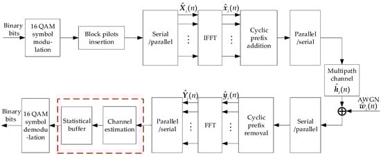
Figure 1.
System model of cyclic prefix (CP)-OFDM. OFDM: orthogonal frequency division multiplexing; QAM: quadrature amplitude modulation; IFFT: inverse fast Fourier transform; FFT: fast Fourier transform.
At the receiver, the CP is removed after the serial to parallel conversion. After removing the CP, the time-domain received OFDM symbols are alternated in the fast Fourier transform (FFT). After that, the frequency-domain OFDM symbols are transformed from the parallel to serial block. The estimated CIR is obtained in the channel estimation block. There are two blocks in the red dashed box: the first one is the channel estimation block, which represents the channel estimation method based on the confidence level; the second one is statistical buffer block, which represents the number of statistical frames . The noise in the multipath channel is further suppressed in the statistical buffer block. At last, the binary information bits are obtained after the 16 QAM symbol demodulation scheme.
4. Block-Type Pilot-Based LS, IMMSE, Threshold Value and Chi-square Distribution Channel Estimation Methods
4.1. Block-Type Pilot-Based LS Channel Estimation Method
After multipath fading and AWGN, the time-domain received OFDM symbols can be represented as:
where represents the cyclic convolution operation and is the frame number. The frequency-domain received OFDM symbols can be represented as:
In the LS channel estimation method, block-type pilots are used to estimate the channel state information. It can be shown that the estimated channel frequency response (CFR) at pilots by the LS method is represented as:
where and are the transmitted and received pilot signals on the -th pilot symbol, is the frequency-domain AWGN on the -th pilot symbol.
After one-dimensional linear interpolation, the estimated CFR is obtained in the entire frequency domain, which can be represented by:
where denotes the channel estimation results for the -th pilot symbol. represents the channel estimation value of the -th pilot symbol. represents the interval between two pilot symbols. The time-domain estimated CIR could be obtained by the IFFT calculation of . Usually, contains time-domain noise , which can be denoted by:
The advantage of block-type pilot-based LS channel estimation is that the channel correlation time is very small, and it is not sensitive to the Doppler effect. The block-type pilot-based LS channel estimation method can be used for mobile reception, and it is simple to design the pattern, easy to implement and saves hardware resources. The disadvantage of the method is that because the interval between pilot points occupies a long time, interpolation filtering cannot accurately reflect the variation of the CIR.
4.2. IMMSE Channel Estimation Method
Through the LS channel estimation in the OFDM receiver, it may not suppress the effect of noise efficiently in the time and frequency domains. The channel response values beyond the length of GI are set to zero to remove the impact of AWGN in this method.
As shown in Figure 1, the CFR obtained by the LS channel estimation method is converted into time-domain CIR with by the IFFT operation. Assuming that is the number of points of GI, the length of CIR should be no longer than that of the GI. To suppress the AWGN effectively, should be considered to be AWGN when . It can be given by:
The cross covariance of and is given by [11]:
where is the operation of complex conjugate transpose. The autocorrelation of is given by [11]:
where is the number of multipaths and is the number of subcarriers. and are the estimated channel and noise variance, respectively. The estimated MMSE CIR could be represented as:
In the dynamic multipath condition, it is difficult to differentiate and . Suppose . In the worst multipath condition, suppose Equation (9) can be represented as:
Suppose . After suppressing the AWGN in time domain, the estimated CIR can be expressed as [15]:
In Equation (11), is the suppression factor, which is usually chosen in the value region of . .
The disadvantage of the IMMSE method in time domain is that it suppresses some paths with small energy as the noise. The IMMSE algorithm involves the multiplication and division operations of points, with large amount of computation and high complexity. Therefore, it is hard to implement in the hardware of the OFDM receiver.
4.3. Threshold Value Channel Estimation Method
The OFDM symbols will be affected by the noise in the wireless channel during the transmission process inevitably. The noise will cause the estimation error of the estimated CIRs and thereby increase the bit error rate (BER) or symbol error rate (SER) performance of the system. Therefore, AWGN is an important factor leading to the decrease of channel estimation accuracy. To suppress the noise and improve the accuracy of channel estimation effectively, many literature works have studied the noise suppression channel estimation methods. The threshold noise suppression method is a commonly-used method in OFDM receivers. The channel estimation method that remains the most significant taps (MST) can suppress noise in the channel estimation results. However, when the number of channels is unknown, the threshold value needs to be set according to the known SNR, so this method is not easy to apply. In the literature [16], the wavelet transform is utilized to estimate the standard deviation of noise; it is used as the threshold value of noise suppression, and the threshold value varies with the change of SNR. The paper proposes the best threshold for computing the noise suppression by optimizing the minimum square error (MSE) of subcarriers, and the threshold value channel estimation results after noise suppression are expressed as [18]:
In Equation (12), is a threshold value that can be defined according to the noise variance . Normally, is set in the threshold region of .
The advantage of the threshold suppression method is that the calculation is simple, but the selection of the threshold will vary with the difference of SNR and channel characteristics. Therefore, the effect of noise suppression is very sensitive to the selection of the threshold. Its disadvantage is that it cannot separate the smaller energy paths from the AWGN in the channel estimation results. That is, it may restore the noise with the larger energy as paths or suppress the paths with small energy as noise. The method of averaging the mean value of the continuous multiple channel estimation results can effectively suppress the noise in the channel estimation results, and the channel estimation method based on the filter matching can also suppress the noise effectively.
4.4. Chi-Square Distribution Channel Estimation Method
The Chi-square distribution channel estimation method can reduce the false alarms caused by AWGN in the estimated CIRs. Reducing the false alarm probability by utilizing the properties of the Chi-square distribution is an efficient way to further improve the accuracy of channel estimation.
The power summation of the -th tap during consecutive frames, i.e., from the -th to the -th frame of the estimated CIR, could be represented as:
The power distribution function (PDF) of satisfies the Chi-square distribution and is given by:
In the literature [15], most of the false alarms in the estimated CIRs can be effectively reduced according to the Chi-square distribution, which can be represented by:
The disadvantage of Equation (15) is that the variance of noise has not been determined in the literature [15]. In order to define the variance of noise accurately, can be represented as:
In the Chi-square distribution channel estimation method, can be chosen from the regions of . The larger the value of is, the higher the accuracy of channel estimation is. In this article, the value of is chosen by odd values to suppress the noise.
5. Channel Estimation Based on Statistical Frames and the Confidence Level
The confidence level shows that the true value of the estimated CIR has a certain probability to fall around the measurement interval. The confidence level gives the credibility of the measured values of the measured CIRs. This probability is called the confidence level. The paper presents an OFDM channel estimation method based on statistical frames and the confidence level, it has good performances in both static and dynamic multipath channels. The method is based on the statistical frames and confidence level . For every consecutive frames, the channel estimation results are counted once. The number of real and imaginary parts , is counted in the intervals of and . Assume the number of times that , which occurs in the intervals of and , is , . The number of times that , which occurs in the intervals of and , is and . The maximum number of , which occurs in the intervals of and , is denoted as . The maximum number of , which occurs in the intervals of and , is denoted as . and can be represented as:
The PDF of noise obeys a Gaussian distribution. The PDF of the Gaussian distribution of noise under different statistical frames is represented in Figure 2. The literature [15] represents the figure of the PDF of the real parts of the path and the noise. The disadvantage is that it does not consider the size of the statistical frames, which could affect the probability of the noise distribution. When the statistical frames increase from five to thirteen, the probability that occurs in the positive and negative intervals may increase.
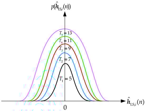
Figure 2.
The probability distribution function of the Gaussian distribution of noise under different statistical frames.
According to the PDF of the Gaussian distribution, if is noise, the number of its real part or imaginary part appears in the positive and negative intervals nearly equal, that is . If is the multipath, the number of the real part or the imaginary part appearing in the statistical interval is approximately equal to the statistical frame number, that is . Therefore, the more is closer to , the higher the confidence level of is; the more is closer to , the lower the confidence level of the is. The confidence level can also be obtained by the soft decision method, which can be represented by:
where are the ranges of confidence level .
Take the maximum of the four values of and is . can be represented as:
Compare with statistical frames . To simplify the calculation of the confidence level, is obtained by using the hard decision method. If is equal to the statistical frames , is one; else, is zero. For example, when the statistical frame is chosen to be five, the confidence level is represented by:
When the statistical frame is chosen to be seven, the confidence level is represented by:
When the statistical frame is chosen to be nine, the confidence level is represented by:
When the statistical frame is chosen to be eleven, the confidence level is represented by:
When the statistical frame is chosen to be thirteen, the confidence level is represented by:
In the confidence level channel estimation method, channel estimation results after noise reduction can be represented as:
The IMMSE channel estimation method needs a large number of multiplication and division arithmetic; therefore, its calculation complexity is higher. The threshold value method may suppress the paths as noise, which induces the reduction of channel estimation precision in the dynamic channels since it is not easy to choose the suitable threshold value. The statistical frames and confidence level based channel estimation method only increases the logic judgment and storage resources, and the computational complexity is low, so it is convenient for hardware implementation.
6. Simulation Results
6.1. The Performance in Static Multipath Channels
The profiles for the China digital television (DTV) Test 1st (CDT1) [18], Brazil A, Brazil B and Brazil D channel models are shown in Table 1 and Table 2, respectively. The Brazil A, Brazil B and Brazil D channels were developed from the Brazilian field test on digital terrestrial television broadcasting (DTTB). The main simulation parameters based on the CP-OFDM system are represented in Table 3. Table 4 proposes a computational complexity comparison of the five channel estimation methods. A simplified radix-two IFFT/FFT approach whose implementation cost is much lower is adopted to process the cyclic convolution operation, and the IFFT/FFT is taken based on 2N points. The five channel estimation methods are based on 2N points division, and is utilized in the proposed CP-OFDM system. The confidence level method only needs T-point addition/subtraction; therefore, it reduces the complexity of hardware implementation largely. This section presents the SER performance comparison between the LS method, the threshold value method, the IMMSE method, the Chi-square distribution method and the confidence level method.

Table 1.
Profiles for the China digital television (DTV) Test 1st (CDT1) and Brazil A multipath fading channels.
Table 2.
Profiles for the Brazil B and Brazil D multipath fading channels.
Table 3.
Simulation parameters of CP-OFDM systems. SPS: symbols per second; CP: cyclic prefix; OFDM: orthogonal frequency division multiplexing; QAM: quadrature amplitude modulation; IMMSE: improved minimum mean square error.
Table 4.
Computational complexity comparison of channel estimation methods. LS: least square; IFFT: inverse fast Fourier transform; FFT: fast Fourier transform.
The conventional LS, IMMSE, threshold value, Chi-square distribution and confidence level methods are presented in the CP-OFDM system. In this paper, statistical OFDM signal frame T is chosen to be 5, 7, 9, 11 and 13 in the CP-OFDM receivers to calculate the confidence level. The modulation mode 16 QAM is chosen to equalize the constellation signals in the receiver of the CP-OFDM system. The length of CP is 180 OFDM subcarriers, and the OFDM symbol consists of 300 subcarriers. In the five channel estimation methods, block-type pilots are inserted in all the subcarriers of the OFDM symbols in the frequency domain. In the simulation, the Doppler spread is chosen to be 20 Hz, 60 Hz and 80 Hz in Brazil A, Brazil B and Brazil D, respectively.
Figure 3 and Figure 4 present the SER performance in the 16 QAM-modulated CP-OFDM system over static CDT1 and Brazil A, respectively. As shown in Figure 3, the gap of the SNR gain among , , and is about 1.5 dB, 0.5 dB and 0.3 dB at the SER of 10−2, respectively.
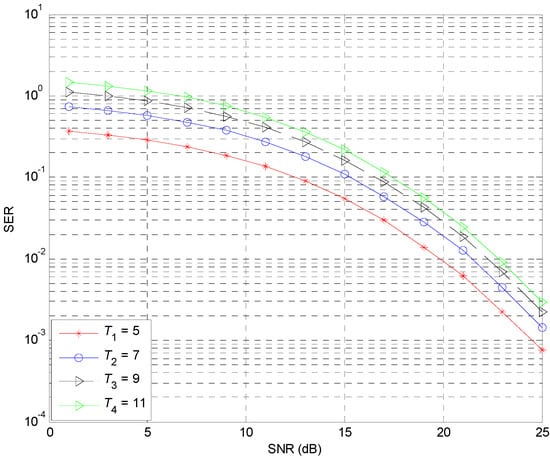
Figure 3.
Symbol error rate (SER) performance of the 16 QAM-modulated CP-OFDM system over static China digital television (DTV) Test 1st (CDT1). SNR: signal-to-noise ratio.
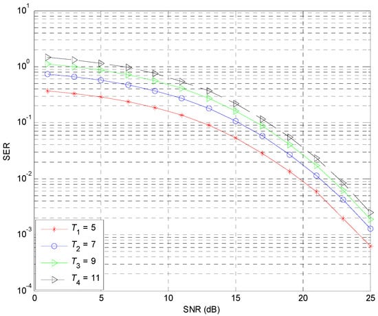
Figure 4.
SER performance of the 16 QAM-modulated CP-OFDM system over static Brazil A.
In Figure 4, the gap of the SNR gain among , , and is about 1.4 dB, 0.8 dB and 0.7 dB at the SER of 10−2, respectively. Therefore, the SER curves of have the best SER gain under the CDT1 and Brazil A multipath fading channels.
Figure 5 presents the SER performance of the proposed confidence level channel estimation method over static CDT1. Compared with the threshold value method, the ideal channel estimation method outperforms the threshold value estimation method with the SNR gains by only about 0.1 dB SNR gains at the target SER of 10–2. The proposed confidence level method outperforms the conventional LS method by about a 1.6 dB SNR gap at the target SER of 10−3. It could be seen that AWGN is the main factor that impacts the accuracy of channel estimation [16].
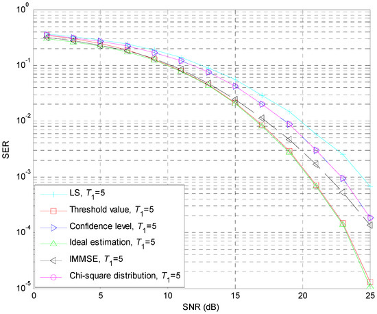
Figure 5.
SER performance of the 16 QAM-modulated CP-OFDM system over static CDT1. LS: least square; IMMSE: improved minimum mean square error.
Under the static CDT1 multipath channel, the threshold value method has the best channel estimation performance since CDT1 belongs to the light frequency selective fading channel. In the static multipath fading condition, the interference caused by noise is relatively small. Therefore, selecting a suitable threshold can remove most of the noise interference in the OFDM receivers. The CDT1 channel has a small amount of side paths. The IMMSE method suppresses the noise while not restraining the energy of the main path; thereby, the IMMSE method has a good channel estimation effect. The SER curve of the confidence level is similar to that of the Chi-square distribution method under static CDT1 since the false alarms obey the Chi-square distribution strictly. Therefore, the SER curves of the proposed confidence level method and Chi-square distribution method can suppress the noise effectively.
6.2. The Performance in Dynamic Multipath Channels
Figure 6 and Figure 7 present the SER performance in 16 QAM-modulated CP-OFDM systems over dynamic Brazil B and Brazil D, respectively. As shown in Figure 6, the gap of the SNR gain among , , and is about 3 dB, 2 dB and 1.2 dB at the SER of 5 × 10⁻², respectively. In Figure 7, the gap of the SNR gain among , , and is about 4 dB, 1.8 dB and 0.5 dB at the SER of 8 × 10⁻², respectively. Therefore, is a suitable value, which can be chosen for the dynamic multipath channels.
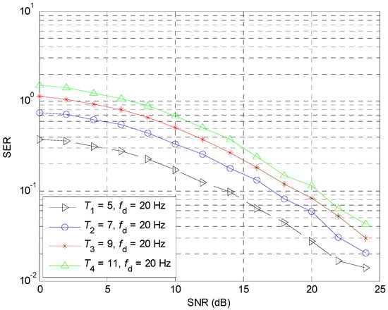
Figure 6.
SER performance of the 16 QAM-modulated CP-OFDM system over Brazil B with a Doppler spread of 20 Hz.
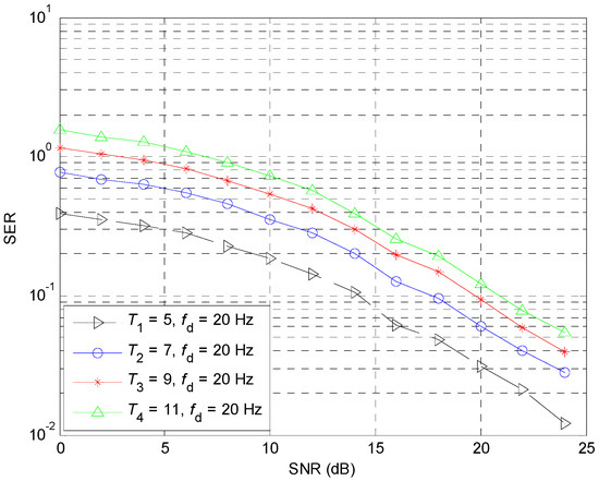
Figure 7.
SER performances of the 16 QAM-modulated CP-OFDM system over Brazil D with a Doppler spread of 20 Hz.
In Figure 8, under the maximum Doppler spread of 20 Hz, the proposed confidence level method can provide 0.4 dB, 1.0 dB and 1.2 dB SNR improvements compared with the IMMSE method, the LS method and the Chi-distribution method at the target SER of 2 × 10⁻², respectively. The IMMSE method has bad SER performance when the SNR is higher than 19 dB. The confidence level method has the best SER performance except the ideal estimation and threshold value methods. As shown in Figure 8, the proposed confidence level method and threshold value method have almost the same SER performance in the lower SNR range. Compared with the ideal channel estimation method, the proposed confidence level method has 2.2 dB SNR degradation at the target SER of 2 × 10⁻².
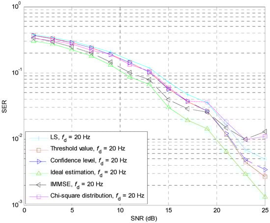
Figure 8.
SER performance of the 16 QAM-modulated CP-OFDM system over Brazil A under .
Under the Brazil B channel with a Doppler spread of 60 Hz, as shown in Figure 9, the proposed confidence level method provides the SNR gains of 0.6 dB, 2.0 dB and 4.5 dB at the SER of 2 × 10⁻² compared with the LS, IMMSE and Chi-square distribution methods, respectively. The IMMSE method has bad SER performance when the SNR is higher than 19 dB. The confidence level method has the best SER performance except the ideal estimation and threshold value methods. Compared with the threshold value method, the proposed confidence level method has 0.4 dB SNR degradation at SER of 2 × 10⁻². Compared with the ideal channel estimation, the proposed confidence level method has 1.9 dB SNR degradation at the target SER of 2 × 10⁻². Furthermore, the SNR gap between the SER performance curves of ideal channel estimation and the proposed confidence level methods is about 1.8 dB at the SER of 2 × 10⁻².
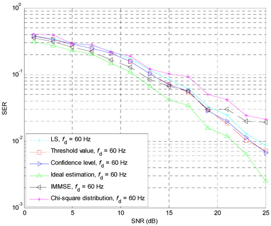
Figure 9.
SER performance of the 16 QAM-modulated CP-OFDM system over Brazil B under .
As shown in Figure 10, compared with the IMMSE method, the Chi-square distribution method and the LS method, the proposed confidence level method provides the SNR gains of 1.3 dB, 1.5 dB and 2.5 dB at the SER of 3 × 10⁻² when the maximum Doppler spread equals 80 Hz. The confidence level method has the best SER performance except the ideal estimation. The IMMSE estimation method has worse SER performance in the high SNR region, and the Chi-square distribution method has the worst SER performance. Compared with the ideal channel estimation, the proposed confidence level method has 2.3 dB SNR degradation at the target SER of 3 × 10⁻². Moreover, compared with the threshold value method, the proposed confidence level method provides the SNR gains of 0.05 dB at the SER of 10−2 with the maximum Doppler spread equal to 80 Hz.
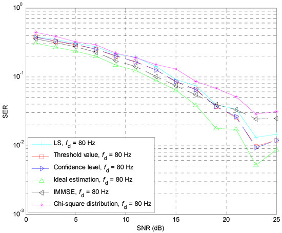
Figure 10.
SER performance of the 16 QAM-modulated CP-OFDM system over Brazil D under .
The proposed confidence level method can suppress the noise effectively based on the statistical frames buffer, which reduces the noise. However, the SER curves are not smooth with Doppler spread equal to 20 Hz, 60 Hz and 80 Hz since the Doppler spread brings interference between adjacent OFDM signals. The 16 QAM utilizing sixteen signals constellations for mapping may cause interference between constellation points under deep fading channels. As the SNR increases, the SER curves still represent a declining trend. The SER performance curves show that the proposed confidence level channel estimation method for the CP-OFDM system is able to provide significant SNR gains under dynamic frequency selective channels.
7. Conclusions
This paper proposes a novel OFDM channel estimation method based on statistical frames and the confidence level. In this paper, it is proven that the proposed channel estimation method can provide good SER performance whenever under the static multipath channels or dynamic multipath channels. When the statistical frame is five, the confidence level channel estimation method has the best SER performance compared to the SER performance with the statistical frame equal to seven, nine and eleven.
Compared with the conventional block-type pilot-based LS, IMMSE, threshold value method and Chi-square distribution method, the proposed confidence level channel estimation method has the best SER performance. The proposed confidence level channel estimation method is easy to implement in hardware and has broad market prospects that can be applied in underwater acoustic communication with multiple-input multiple-output (MIMO) technology [19], RAKE receiving technology [20] and frequency hopping technology [21,22].
Author Contributions
X.Z. and C.W. conceived of the algorithm and designed the experiments. X.Z. and R.T. performed the experiments. X.Z. and C.W. analyzed the results. X.Z. and C.W. drafted the manuscript. X.Z., C.W., R.T. and M.Z. revised the manuscript. All authors read and approved the final manuscript.
Funding
This research was funded by the National Natural Science Foundation of China (Grant No. 61702303) and the Shandong Provincial Natural Science Foundation, China (Grant Nos. ZR2017MF020 and ZR2015PF004).
Conflicts of Interest
The authors declare no conflict of interest.
References
- Zhang, X.J.; Yuan, Z.T. The application of interpolation algorithms in OFDM channel estimation. Int. J. Simul. Syst. Sci. Technol. 2016, 17, 11.1–11.5. [Google Scholar]
- Ding, W.B.; Yang, F.; Song, J. Out-of-band power suppression for TDS-OFDM systems. In Proceedings of the IEEE International Symposium on Broadband Multimedia Systems and Broadcasting, London, UK, 5–7 June 2013. [Google Scholar]
- Wang, G.P.; Gao, F.F.; Zhang, X.; Tellambura, C. Superimposed training-based joint CFO and channel estimation for CP-OFDM modulated two-way relay networks. EURASIP J. Wirel. Commun. Netw. 2010, 403936. [Google Scholar] [CrossRef]
- Wang, G.P.; Gao, F.F.; Wu, Y.-C.; Tellambura, C. Joint CFO and channel estimation for ZP-OFDM modulated two-way relay networks. In Proceedings of the IEEE Wireless Communication and Networking Conference, Sydney, NSW, Australia, 18–21 April 2010. [Google Scholar]
- Wang, S.; Manton, J.H. Blind channel estimation for non-CP OFDM systems using multiple receive antennas. IEEE Signal Process. Lett. 2009, 16, 299–302. [Google Scholar] [CrossRef]
- Inserra, D.; Tonello, A.M. Training symbol exploitation in CP-OFDM for DoA estimation in multipath channels. In Proceedings of the 21st European Signal Processing Conference, Marrakech, Morocco, 9–13 September 2013. [Google Scholar]
- Hu, S.; Wu, G.; Yang, G.; Li, S.Q.; Gao, B. Effectiveness of preamble based channel estimation for OFDM/OQAM system. In Proceedings of the International Conference on Networks Security, Wireless Communications and Trusted Computing, Wuhan, China, 25–26 April 2009. [Google Scholar]
- Khan, A.M.; Jeoti, V.; Zakariya, M.A. Improved pilot-based LS and MMSE channel estimation using DFT for DVB-T OFDM systems. In Proceedings of the IEEE Symposium on Wireless Technology & Applications, Kuching, Malaysia, 22–25 September 2013. [Google Scholar]
- Al-Ogaili, F.; Elayan, H.; Alhalabi, L.; Al-Shabili, A.; Taha, B.; Weruaga, L.; Jimaa, S. Leveraging the ℓ1-LS criterion for OFDM sparse wireless channel estimation. In Proceedings of the 11th IEEE International Conference on Wireless and Mobile Computing, Networking and Communications, Abu Dhabi, UAE, 19–21 October 2015. [Google Scholar]
- Khan, L.U.; Khan, N.; Khattak, M.I.; Shafi, M. LS estimator: Performance analysis for block-type and comb-type channel estimation in OFDM system. In Proceedings of the 11th International Bhurban Conference on Applied Sciences and Technology, Islamabad, Pakistan, 14–18 January 2014. [Google Scholar]
- Sutar, M.B.; Patil, V.S. LS and MMSE estimation with different fading channels for OFDM system. In Proceedings of the International Conference on Electronics, Communication and Aerospace Technology, Coimbatore, India, 20–22 April 2017. [Google Scholar]
- Ohno, S.; Munesada, S.; Manasseh, E. Low-complexity approximate LMMSE channel estimation for OFDM systems. In Proceedings of the Asia-Pacific Signal and Information Processing Association Annual Summit and Conference, Hollywood, CA, USA, 3–6 December 2012. [Google Scholar]
- Tong, Z.R.; Guo, M.J.; Yang, X.F.; Zhang, W.H. Performance comparison of LS and LMMSE channel estimation algorithm for CO-OFDM system. In Proceedings of the 3rd International Conference on Mechanical and Electronics Engineering, Hefei, China, 23–25 September 2011. [Google Scholar]
- Tang, R.G.; Zhou, X.; Wang, C.Y. A novel low rank LMMSE channel estimation method in OFDM systems. In Proceedings of the 17th IEEE International Conference on Communication Technology, Chengdu, China, 27–30 October 2017. [Google Scholar]
- Zhou, X.; Yang, F.; Song, J. A novel noise suppression method in channel estimation. IEICE Transac. Fundam. Electron. Commun. Comput. Sci. 2011, E94-A, 2027–2030. [Google Scholar] [CrossRef]
- Zhou, X.; Ye, Z.; Liu, X.X.; Wang, C.Y. Channel estimation based on linear filtering least square in OFDM systems. J. Commun. 2016, 11, 1005–1011. [Google Scholar] [CrossRef]
- Zhou, X.; Ye, Z.; Liu, X.X.; Wang, C.Y. Chi-square distribution-based confidence measure channel estimation method in OFDM Systems. IETE J. Res. 2017, 63, 662–670. [Google Scholar] [CrossRef]
- Tang, R.G.; Zhou, X.; Wang, C.Y. A Haar wavelet decision feedback channel estimation method in OFDM systems. Appl. Sci. 2018, 8, 877. [Google Scholar] [CrossRef]
- Han, X.; Yin, J.W.; Yu, G. Multiple-input multiple-output under-ice acoustic communication in shallow water. In Proceedings of the 11th ACM International Conference on Underwater Networks and Systems, Shanghai, China, 24–26 October 2016. [Google Scholar]
- Yoshizawa, S.; Tanimoto, H.; Saito, T. Experimental results of OFDM rake reception for shallow water acoustic communication. In Proceedings of the Techno-Ocean 2016: Return to the Oceans, Kobe, Japan, 6–8 October 2016. [Google Scholar]
- Yang, T.C. Properties of underwater acoustic communication channels in shallow water. J. Acoust. Soc. Am. 2012, 131, 129–145. [Google Scholar] [CrossRef] [PubMed]
- Lv, S.; Shen, X.H. Research on shallow water acoustic communication based on frequency hopping. In Proceedings of the IEEE International Conference on Signal Processing, Communications and Computing, Hong Kong, China, 12–15 August 2012. [Google Scholar]
© 2018 by the authors. Licensee MDPI, Basel, Switzerland. This article is an open access article distributed under the terms and conditions of the Creative Commons Attribution (CC BY) license (http://creativecommons.org/licenses/by/4.0/).