Measurements of High-Frequency Atmospheric Turbulence and Its Impact on the Boundary Layer of Wind Turbine Blades


Abstract
1. Introduction
2. Measurements
3. Analysis
- The surface is colder than the fluid and the gradient becomes and therefore, . Heat is transported by conduction only, and a convection flow does not occur. In this case, the stratification is strong, and turbulence gets damped. The boundary condition is stable for .
- The temperature gradient is zero and therefore, . There is no temperature gradient and therefore, no conduction nor convection. This condition is called neutral.
- The surface is warmer than the fluid and the gradient becomes and therefore, . Heat is transported by conduction and by convection from the surface to the fluid. The convection results in a vertical, upward component of the flow that interacts with the horizontal velocity component. This leads to the production of turbulence in the boundary layer and therefore, is called unstable.
4. Results
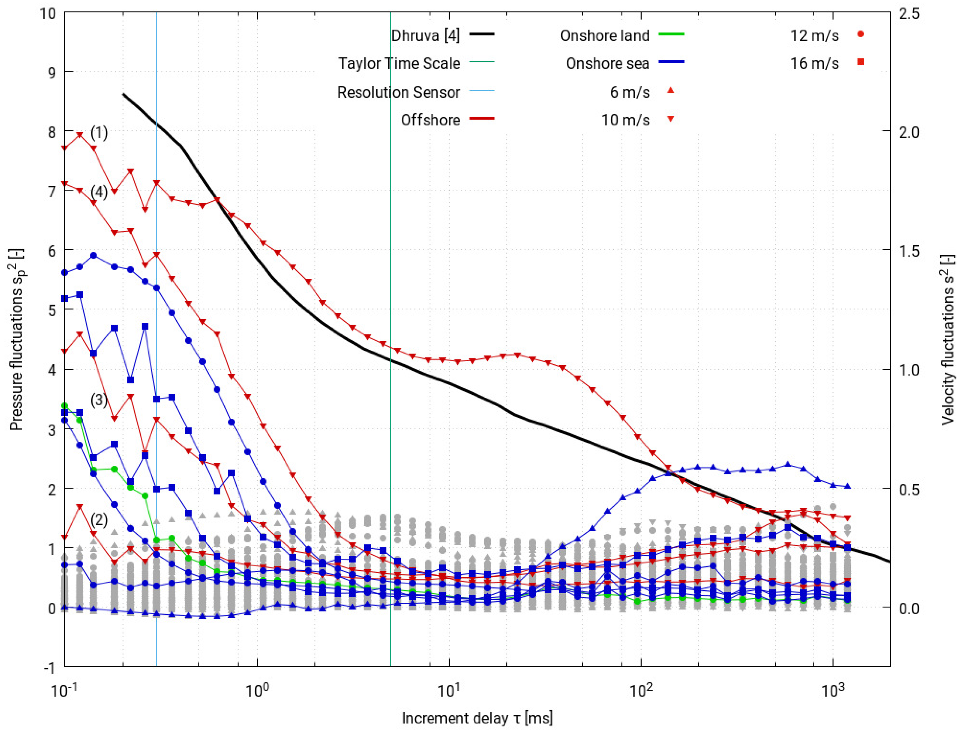
- (1)
- 19 October 2010, 8:44 a.m.
- (2)
- 19 October 2010, 8:54 a.m.
- (3)
- 19 October 2010, 8:55 a.m.
- (4)
- 19 October 2010, 8:57 a.m.
4.1. Time Development of a Sample Time Series
4.2. Occurrence Probabilities
4.3. Confidence Considerations
5. Impact on Boundary Layer Transition on a Wind Turbine Blade
6. Conclusions
Author Contributions
Funding
Acknowledgments
Conflicts of Interest
References
- Schaffarczyk, A. (Ed.) Understanding Wind Power Technology; Wiley: Chichester, UK, 2014. [Google Scholar]
- Schaffarczyk, A.P. Introduction to Wind Turbine Aerodynamics; Springer: Berlin, Germany, 2014. [Google Scholar]
- Emeis, S. Wind Energy Meteorology; Springer: Heidelberg, Germany, 2013. [Google Scholar]
- Obukhov, A.M. Turbulence in an atmosphere with a non-uniform temperature. Bound.-Lay. Metereol. 1971, 2, 7–29. [Google Scholar] [CrossRef]
- Kaimal, J.; Finnigan, J. Atmospheric Boundary Layer Flows: Their Structure and Measurements; Oxford University Press: Oxford, UK, 1994. [Google Scholar]
- Mahrt, L.; Vickers, D.; Howell, J.; Høstrup, J.; Wilzak, J.; Edson, J.; Hare, J. Sea surfuace drag coeficiecient in the Risøe Air Sea Experiment. J. Geophys. Res. 1996, 14, 327–335. [Google Scholar]
- Grachev, A.; Leo, L.; Fernando, H.; Fairall, C.; Creegan, E.; Blomquist, B.W.; Christman, A.; Hocut, C. Air-sea/land interaction in the costal zone. Bound.-Lay. Meteorol. 2018, 167, 181–210. [Google Scholar]
- Reeh, A.D.; Weissmüller, M.; Tropea, C. Free-Flight Investigation of Transition under Turbulent Conditions on a Laminar Wing Glove. In Proceedings of the 51st AIAA Aerospace Sciences Meeting, Grapevine, TX, USA, 7–10 January 2013. [Google Scholar]
- Reeh, A.D.; Tropea, C. Behaviour of a natural laminar flow airfoil in flight through atmospheric turbulence. J. Fluid Mech. 2015, 767, 394–429. [Google Scholar] [CrossRef]
- Schaffarczyk, A.; Schwab, D.; Breuer, M. Experimental detection of Laminar-Turbulent Transition on a rotating wind turbine blade in the free atmosphere. Wind Energy 2016, 19. [Google Scholar] [CrossRef]
- Schwab, D. Aerodynamische Grenzschichtuntersuchungen an Einem Windturbinenblatt im Freifeld. Ph.D. Thesis, Helmut-Schmidt-Universität, Hamburg, Germany, 2018. [Google Scholar]
- Beck, C. Superstatistics in hydrodynamic turbulence. Physica D 2004, 193, 195–207. [Google Scholar] [CrossRef]
- Castaing, B.; Gagne, Y.; Hopfinger, E. Velocity probability density functions of high Reynolds number turbulence. Physica D 1990, 64, 177–200. [Google Scholar] [CrossRef]
- Jeromin, A.; Schaffarczyk, A.P. Advanced statistical analysis of high-frequency turbulent pressure fluctuations for on- and off-shore wind. In Proceedings of the EUROMECH Colloquium 528: Wind Energy and the Impact of Turbulence on the Conversion Process, Oldenburg, Germany, 22–24 February 2012. [Google Scholar]
- Jeromin, A.; Schaffarczyk, A.P. Relating high-frequency offshore turbulence statistics to boundary layer stability. In Proceedings of the 2013 International Conference on Aerodynamics of Offshore Wind Energy Systems and Wakes (ICOWES2013), Frankfurt, Germany, 19–21 November 2013; Shen, W.Z., Ed.; 2013; pp. 162–172. [Google Scholar]
- Segalini, A.; Ramis, O.; Schlatter, P.; Henrik Alfredsson, P.; Rüedi, J.D.; Alessandro, T. A method to estimate turbulenFphysicace intensity and transvers Taylor microscale in turbulent flows from spatially averaged hot-wire data. Exp. Fluids 2011, 51, 693–700. [Google Scholar] [CrossRef]
- Jeromin, A.; Schaffarczyk, A.P. Statistische Auswertungen Turbulenter Druckfluktuationen auf der Off-Shore Messplattform FINO3; Technical Report Unpublished Interal Report No. 78; University of Applied Sciences Kiel: Kiel, Germany, 2012. [Google Scholar]
- Lück, S.; Renner, C.; Peinke, J.; Friedrich, R. The Markov-Einstein coherence length—An new meaning for the Taylor length in turbulence. Phys. Lett. 2006, 359, 335–338. [Google Scholar] [CrossRef]
- Batchelor, G. Pressure fluctuations in isotropic turbulence. Proc. Camb. Philos. Soc. 1951, 47, 359–374. [Google Scholar] [CrossRef]
- Xu, H.; Ouellette, T.; Vincenzi, D.; Bodenschatz, B. Acceleration correlations and pressure structure functions in high-reynolds number turbulence. Phys. Rev. Lett. 2007, 99, 204501. [Google Scholar] [CrossRef] [PubMed]
- Sathe, M.; Mann, J.; Barlas, T.; Bierbooms, W.; van Bussel, G. Influence of atmospheric stability on wind turbine loads. Wind Energy 2013, 16, 1013–1032. [Google Scholar] [CrossRef]
- Coelingh, J.; van Wijk, A.; Holtslag, A. Analysis of wind speed observations over the North Sea. J. Wind Eng. Ind. Aerodyn. 1996, 61, 51–69. [Google Scholar] [CrossRef]
- Oost, W.; Jacobs, C.; van Oort, C. Stability effects on heat and moisture fluexes at sea. Bound.-Lay. Meteorol. 2000, 95, 271–302. [Google Scholar] [CrossRef]
- Emeis, S. Upper limit for wind shear instable stratified conditions expressed in terms of a bulk Richardson number. Meteorol. Z. 2017, 16, 421–430. [Google Scholar] [CrossRef]
- Dhruva, B. An Experimental Study of High Reynolds Number Turbulence in the Atmosphere. Ph.D. Thesis, Yale University, New Haven, CT, USA, 2000. [Google Scholar]
- Jeromin, A.; Schaffarczyk, A.; Puczylowski, J.; Peinke, J.; Hoelling, M. Highy resolved measurements of atmospheric turbulence with the new 2D-atmospheric Laser Cantilever Anemometer. J. Phys. Conf. Ser. 2014, 555. [Google Scholar] [CrossRef]
- Lohse, D.; Grossmann, S. Intermittency in turbulence. Physica A 1993, 194, 519–531. [Google Scholar] [CrossRef]
- Madsen, H.; Fuglsang, P.; Romblad, J.; Enevoldsen, P.; Laursen, J.; Jensen, L.; Bak, C.; Paulsen, U.S.; Gaunna, M.; Sorensen, N.N.; et al. The DAN-AERO MW experiments. AIAA 2010, 645. [Google Scholar] [CrossRef]
- Batchelor, G. An Introduction to Fluid Dynamics; Cambridge University Press: Cambridge, UK, 1967. [Google Scholar]


| Date & Time | Location | (m/s) | Ti (%) | Ri (-) | Boundary Layer State | |
|---|---|---|---|---|---|---|
| 21 October 2010, 7:56 a.m. | Offshore | 06.6 | 08.2 | −0.54 | Unstable | |
| 28 April 2008, 9:35 a.m. | Onshore | 06.1 | 11.9 | −0.15 | Unstable | |
| 19 October 2010, 8:57 a.m. | Offshore | 10.8 | 02.2 | −0.13 | Unstable | * |
| 19 October 2010, 8:44 a.m. | Offshore | 10.2 | 03.1 | −0.12 | Unstable | * |
| 19 August 2010, 8:13 a.m. | Offshore | 12.7 | 02.8 | −0.06 | Unstable | |
| 25 March 2008, 2:55 p.m. | Onshore | 11.3 | 10.8 | −0.03 | Unstable | * |
| 29 March 2008, 11:44 a.m. | Onshore | 15.3 | 10.6 | −0.01 | Neutral | |
| 30 March 2008, 6:04 p.m. | Onshore | 15.7 | 05.6 | 00.00 | Neutral | * |
| 28 April 2008, 2:20 p.m. | Onshore | 05.8 | 02.1 | 00.01 | Neutral | * |
| 1 May 2008, 2:55 a.m. | Onshore | 06.0 | 06.0 | 00.10 | Stable | |
| 12 April 2008, 7:24 p.m. | Onshore | 05.2 | 11.0 | 00.28 | Stable |
| Time | (K) | (K) | (m/s) | Ti (%) | Ri (-) | Boundary Layer State | |
|---|---|---|---|---|---|---|---|
| 8:44 a.m. | 283.6 | 286.8 | 10.2 | 03.1 | −0.12 | Unstable | * |
| 8:45 a.m. | 283.5 | 286.8 | 10.2 | 03.9 | −0.13 | Unstable | |
| 8:47 a.m. | 283.4 | 286.8 | 10.0 | 07.5 | −0.14 | Unstable | |
| 8:49 a.m. | 283.4 | 286.8 | 10.1 | 07.3 | −0.13 | Unstable | |
| 8:50 a.m. | 283.5 | 286.8 | 09.3 | 06.7 | −0.16 | Unstable | |
| 8:52 a.m. | 283.5 | 286.8 | 11.2 | 06.0 | −0.11 | Unstable | |
| 8:54 a.m. | 283.5 | 286.8 | 10.8 | 07.7 | −0.11 | Unstable | * |
| 8:55 a.m. | 283.2 | 286.8 | 11.2 | 04.2 | −0.12 | Unstable | * |
| 8:57 a.m. | 283.1 | 286.8 | 10.8 | 02.2 | −0.13 | Unstable | * |
| Boundary Layer State | ||||
|---|---|---|---|---|
| Unstable | Neutral | Stable | Total | |
| All | 84.0 | 23.0 | 12.0 | 119.0 |
| Offshore | 65.0 | 00.0 | 00.0 | 065.0 |
| Onshore | 19.0 | 23.0 | 12.0 | 054.0 |
| All | 07.0 | 04.0 | 00.0 | 011.0 |
| Probability (%) | 08.3 | 17.4 | 00.0 | 009.2 |
| Offshore | 04.0 | 00.0 | 00.0 | 004.0 |
| Probability (%) | 06.2 | -/- | -/- | 0-/- |
| Onshore | 03.0 | 04.0 | 00.0 | 007.0 |
| Probability (%) | 15.8 | 17.4 | 00.0 | 0-/- |
| Hypotheses: | |
|---|---|
| Occurrence probability is in stable conditions | |
| Occurrence probability is in stable conditions | |
| Error Type I | |
| Number of samples | 12 |
| Occurrence probability | |
| Expected occurrences | |
| Variance | |
| Acceptance region for | {1…12} |
| Rejection region for | {0} |
| Probability of error | 11.2% |
| Hypotheses: | ||
|---|---|---|
| Occurrence probability is in unstable/neutral conditions | ||
| Occurrence probability is in unstable/neutral conditions | ||
| Error Type I | Error Type II | |
| Number of samples | 42 | |
| Occurrence probability | ||
| Expected occurrences | ||
| Variance | ||
| Acceptance region for | {0…4} | |
| Rejection region for | {5…42} | |
| Probability of error | 11.4% | 14.9% |
© 2018 by the authors. Licensee MDPI, Basel, Switzerland. This article is an open access article distributed under the terms and conditions of the Creative Commons Attribution (CC BY) license (http://creativecommons.org/licenses/by/4.0/).
Share and Cite
Schaffarczyk, A.P.; Jeromin, A. Measurements of High-Frequency Atmospheric Turbulence and Its Impact on the Boundary Layer of Wind Turbine Blades. Appl. Sci. 2018, 8, 1417. https://doi.org/10.3390/app8091417
Schaffarczyk AP, Jeromin A. Measurements of High-Frequency Atmospheric Turbulence and Its Impact on the Boundary Layer of Wind Turbine Blades. Applied Sciences. 2018; 8(9):1417. https://doi.org/10.3390/app8091417
Chicago/Turabian StyleSchaffarczyk, Alois Peter, and Andreas Jeromin. 2018. "Measurements of High-Frequency Atmospheric Turbulence and Its Impact on the Boundary Layer of Wind Turbine Blades" Applied Sciences 8, no. 9: 1417. https://doi.org/10.3390/app8091417
APA StyleSchaffarczyk, A. P., & Jeromin, A. (2018). Measurements of High-Frequency Atmospheric Turbulence and Its Impact on the Boundary Layer of Wind Turbine Blades. Applied Sciences, 8(9), 1417. https://doi.org/10.3390/app8091417