2.1. Sitting Posture Classification
Several methods have been adopted to measure sitting posture and classify it. Camera, is one of the method used to identify and capture sitting postures [
22]. Sensors can also be used by being attached to the user’s back to recognize sitting postures based on motion data [
23,
24,
25]. However, the former introduces issues with respect to privacy and unnatural behavior owing to negative feelings caused by being monitored [
26], and the latter has drawbacks of the possibility of inducing unnatural movements owing to the attached sensors [
27]. The use of pressure sensors mounted on the parts of a chair (e.g., seat and backrest) has been employed to classify sitting postures to overcome these issues. Previous studies have been performed for classifying sitting postures of users by attaching pressure sensors to chair structures such as the seat and backrest as a method to overcome the aforementioned issues.
Table 1 shows the previous studies in which posture classification was performed, including the number of pressure sensors used, the locations in which they were installed, participant information, the number of predicted sitting conditions, the algorithm used, and the overall accuracy.
Although the number of sensors used in previous studies varied, these studies can be largely divided into two types depending on the location of installation of the sensor. In one type, the sensor was attached to the seat only [
26,
28,
29], and in the other type the sensor was attached to both the seat and backrest [
9,
30,
31,
32]. In addition to the pressure sensor, Benocci et al. [
8] used additional sensors such as kinetic related and temperature sensors to classify the sitting postures. Most of the previous studies attempted to classify the sitting upright posture in which the waist is straight, and the feet are placed flat on the floor, the postures in which the upper body is tilted forward, backward, left, or right, and the postures in which the left or right leg is crossed. In the case of the classification of various other postures, the postures in which the legs are crossed were segmented (e.g., one leg over the other, one leg over the other with one foot on the other, one foot on the seat under the other leg’s thigh) [
32]. In addition, there were also cases wherein the movement pattern of the upper body and whether the user was seated were predicted [
28,
31]. Various methods have been adopted for classifying the sitting postures, and they include the use of PCA [
32], Naïve Bayes classifier [
10], hybrid cascade sitting posture classifier [
30], SVM [
29,
33], kNN [
9], dynamic time warping-based classification [
26], and density-based methods [
28]. Ma et al. [
30] have compared the classification performance obtained on applying DT, SVM, and multilayer perception.
2.2. Learning Algorithm
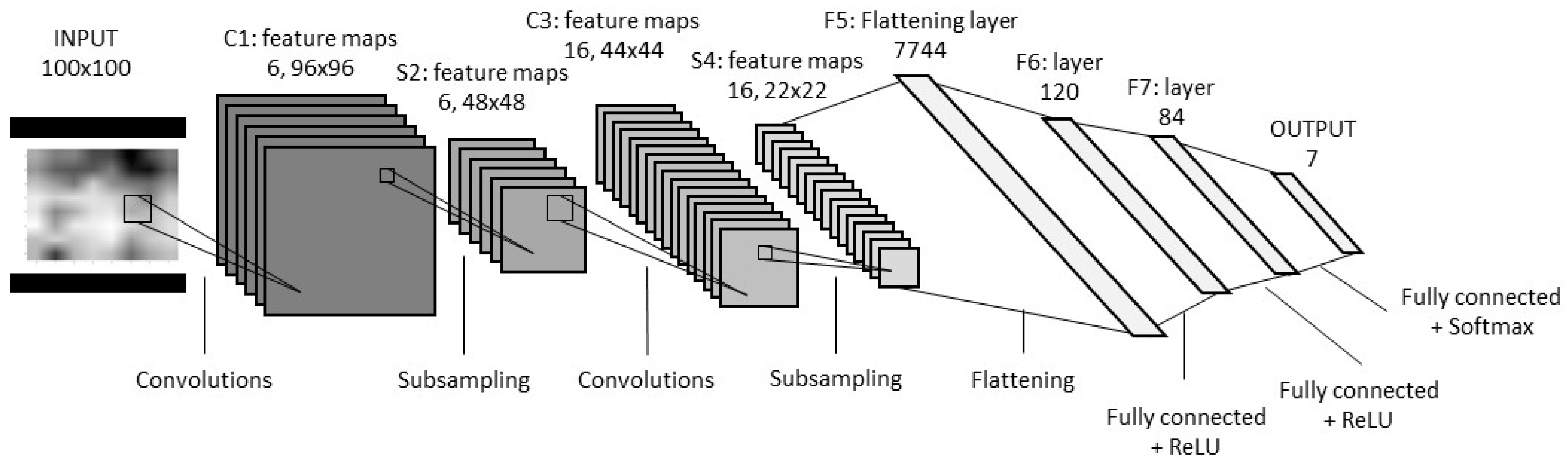
The LeNet-5 which is one of the early CNN model proposed by LeCun for use in character recognition is specialized in adaptive image processing [
34]. CNN is easier to train than other types of feedforward artificial neural network techniques and has the advantage of using fewer parameters. For this reason, CNN has been applied in various fields [
35,
36,
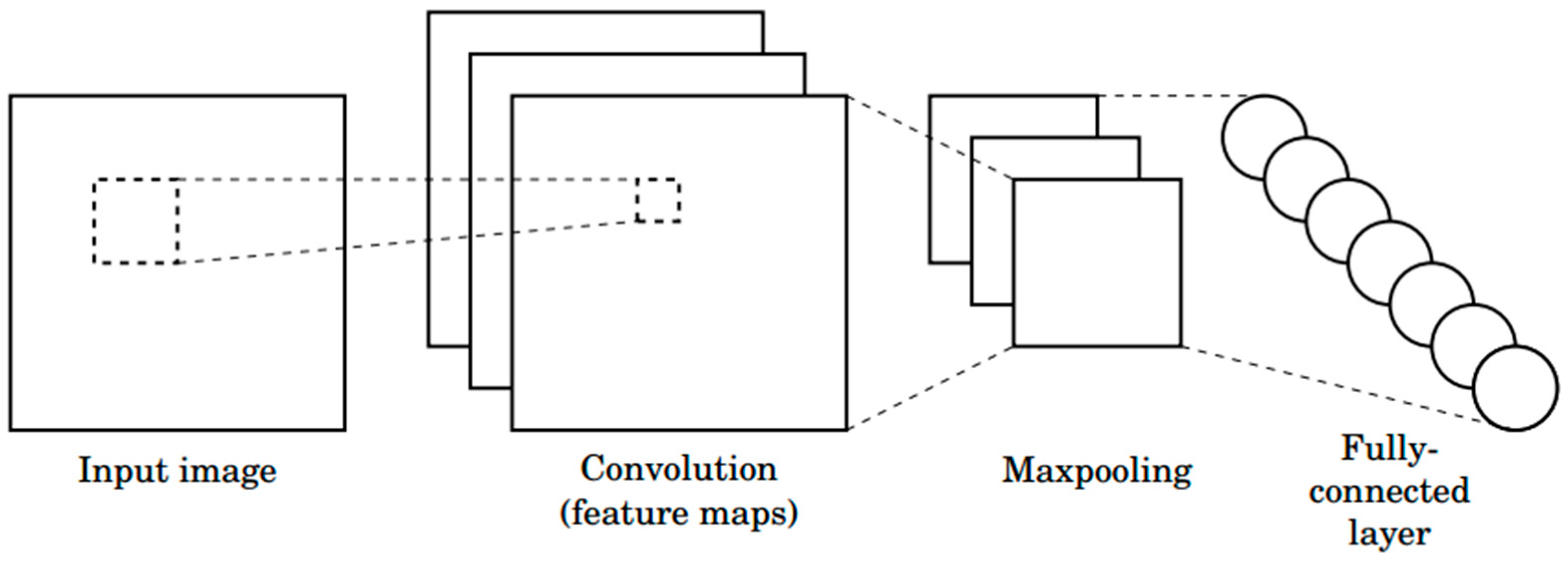
37]. The structure of a common CNN is shown in
Figure 1. It consists of a series of layers. Each layer contains one or more planes. Each plane receives inputs from a small neighborhood in the plane of the previous layer. Each plane can be viewed as a feature map with a fixed feature detector that is convolved to a local window that retrieves the plane from the previous layer. Multiple layers are used on each layer to detect multiple features. The layer is called the convolutional layer. Once the feature is detected, the exact location becomes less important. As a result, the convolutional layer typically follows a different layer that typically performs local averages and sub-samples operations. These layers are referred to as sub-sample layers. Finally, the network has a fully connected network that performs cataloguing operations using features extracted from the previous layer. The network was uniformly trained by a backpropagation algorithm.
The NB classifier is a supervised machine learning classifier, and it is a probabilistic classification algorithm based on the Bayes theorem. In this model, it is generally assumed that all attributes are independent of each other, given the class [
38] and it is widely adopted to reduce the number of parameters. Equations (1)–(3) represent the Bayes rule, assumption of conditional independence, and classification rule for the new input data. According to Zhang [
39], less training data is required to accurately estimate the parameters required for the classification as compared to other complex graphical models.
The multinomial logistic regression (MLR) classifier was introduced by McFadden, and it is a classification method that can be used to predict more than two possible discrete variables [
40]. Similar to binary logistic regression, the probability of categorical membership is evaluated based on the maximum likelihood estimation. In addition, this model does not assume normality, linearity, or homoscedasticity [
41].
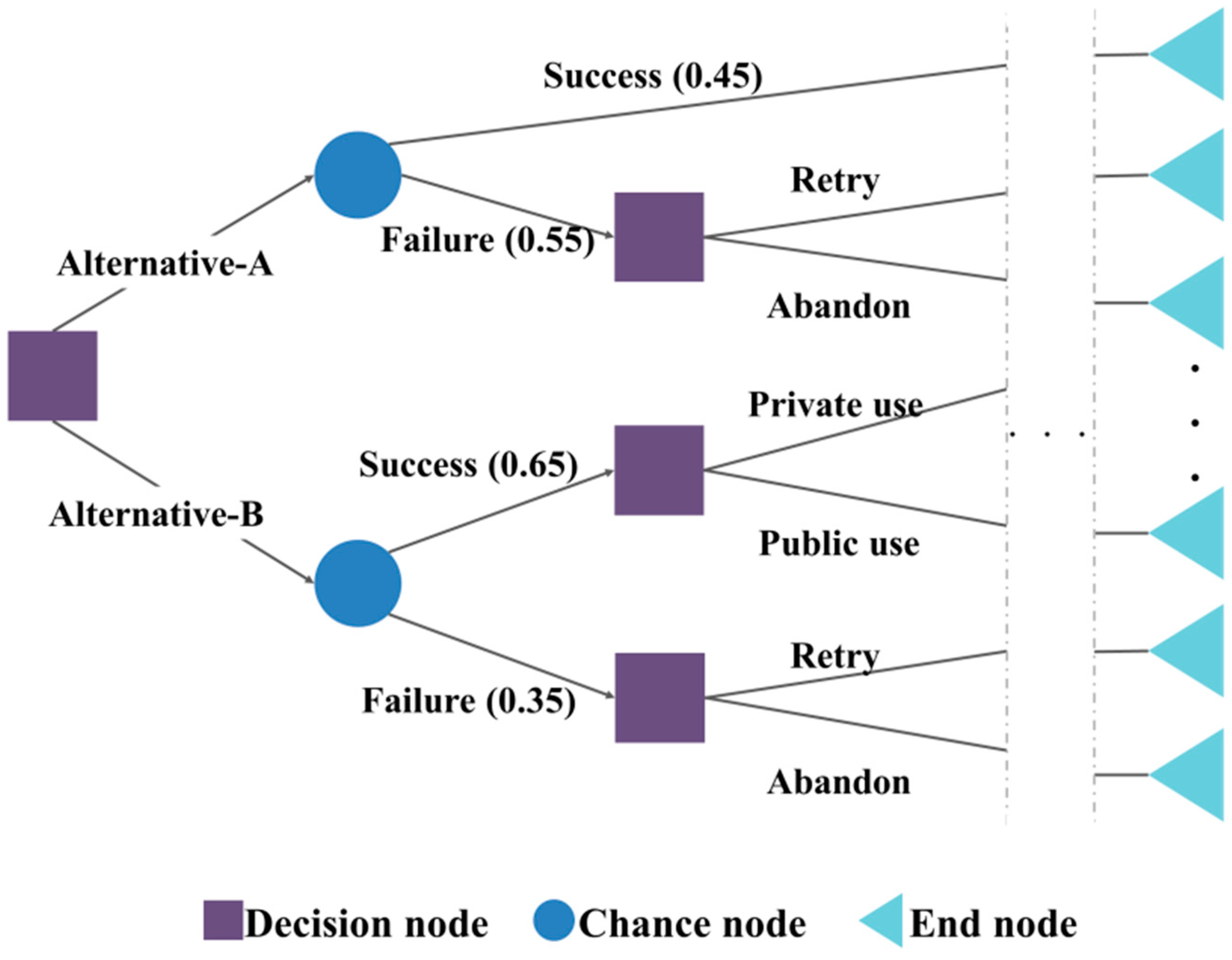
The DT method is a regression analysis or classification method depending on whether the response variable is continuous or categorical. The DT learning algorithm was developed by Quinlan to construct decision tree from an obtained data set [
42]. This model divides the space of the predictive variables and predicts the values of the dependent variables in the divided parts. The formation process of this model mainly consists of growth, pruning, feasibility assessment, interpretation, and forecasting. This algorithm forms a tree-like structure based on separation criterion concerning an impurity index such as entropy and the Gini index. According to Kamiński [
43], this model consists of three types of nodes, which are the decision, chance, and end nodes. An example of a typical structure of this model is presented in
Figure 2.
The NN is a statistical learning algorithm that is inspired by neural networks of the brain, which is an animal’s central nervous system [
44]. To realize an acceptable performance, this model requires the use of a large number of interconnected neurons [
45]. Generally, models of NNs are divided into feed forward NNs and recurrent NNs in terms of signaling schemes. The representative structure of this model is presented in
Figure 3.
The output value of each node is calculated as follows:
where
N is a dimension of the input vector,
X is a value of the input, and
W is the weight value. A function
σ (∙) is a sigmoid activation function, which facilitates expansion to a nonlinear model. A logistic function, hyperbolic tangent function, or probit function is commonly used as the activation function. In the training process, this algorithm determines the optimization weight value
Wi. In a typical NN model consisting of multiple layers, the output value of the
kth node in the
nth layer is described as follows:
where
σ is the activation function.
Wikn is the weight value connected from the
jth node of the
n − 1th layer to the
kth node of the
nth layer. The output value derived from the
jth node of the
n − 1th layer serves as an input value. The weights are usually found by using the backpropagation method during the learning phase.
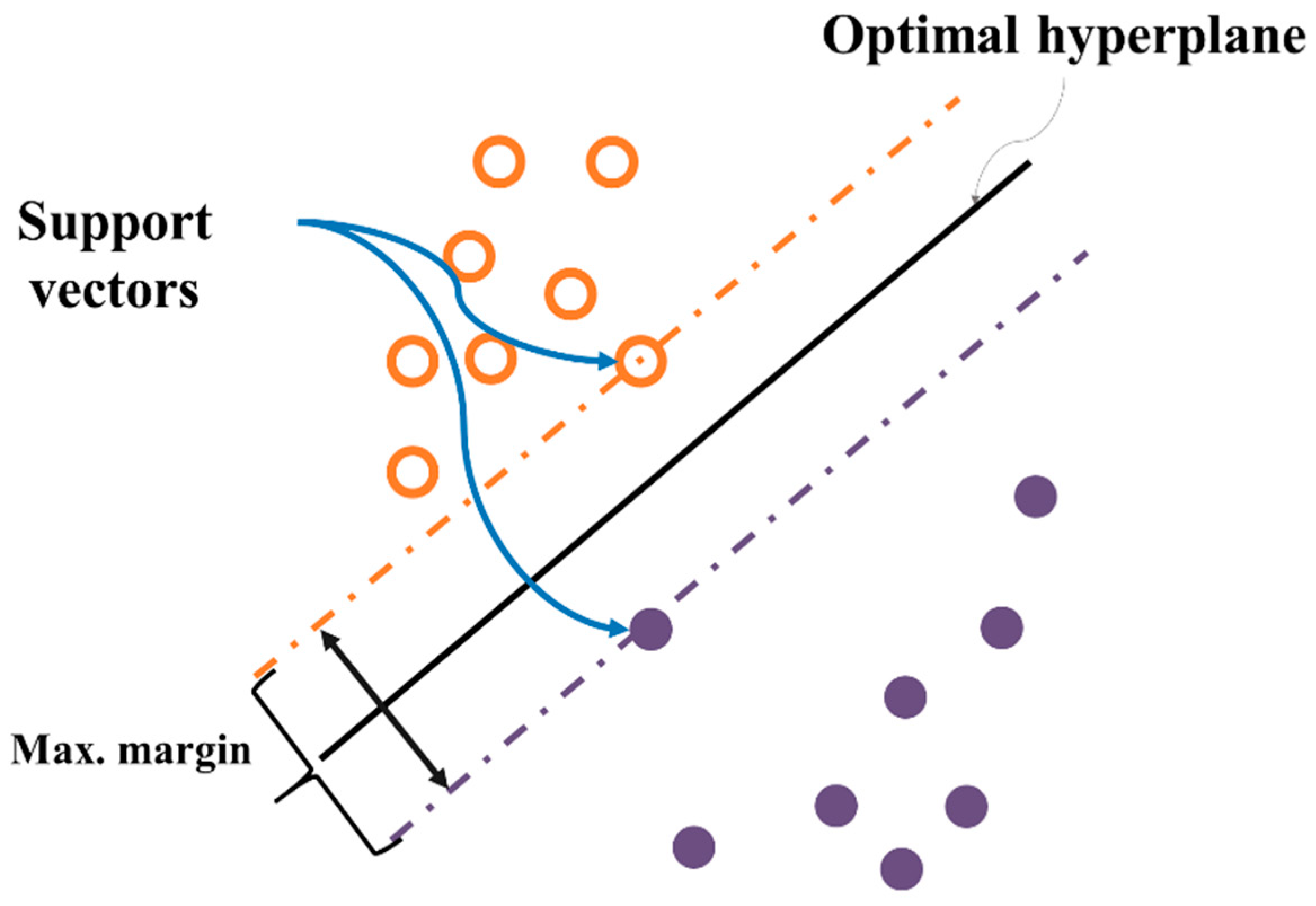
The SVM is a supervised learning model for pattern recognition and data analysis. It is mainly used for classification and regression analysis [
46]. This algorithm finds a classifying hyperplane that can maximize margins in the feature space wherein the original data is mapped [
47]. By solving the dual problem of the original optimization, it is only required to calculate the kernel function values,
, the inner product of feature vectors instead of feature vectors themselves, where
is a mapping function from the original space to the feature space.
This characteristic dramatically increases flexibility of the mapping function and reduces computational cost. For example, the Gaussian (radial basis) kernel function,
with the kernel scaling factor
, can be employed to construct SVM models although the corresponding feature vector
cannot be explicitly calculated because it is represented as an infinite dimensional vector. The representative structure of this model is presented in
Figure 4. Both one versus one extension and one versus all extension are generally employed to extend the binary classification task to multiclass classification tasks for SVM. For more details on SVM, please see [
47].


