1. Introduction
In the past two decades, the development of state-of-the-art technologies for generating and controlling ultra-short intense laser pulses has paved the way for more profound insights into electron and nuclear dynamics in atoms and molecules on their natural timescales [
1,
2,
3,
4,
5]. Current theoretical treatments largely focus on electronic dynamics. However, recent experiments have demonstrated the retrieval of bond distances in simple diatomic molecules [
6] and control over the ultrafast dissociation process and resolution of bond dynamics of a polyatomic molecule using laser-induced electron diffraction (LIED) [
7]. To fully understand molecular dynamics during interaction with a strong laser pulse, it is therefore essential to develop a theory that takes into account the bond dynamics and dissociation process and thereby accurately describes nuclear, as well as electronic, motion. This is the aim of the present work.
Among a wide variety of computational methods, one of the most applicable and important approaches is the direct solution of the time-dependent Schrödinger equation (TDSE). This approach is implementable for simulating systems with a limited number of particles in a limited region of momentum or coordinate space. There are different TDSE approaches for simulating the electron dynamics in an atomic or molecular laser-induced system in one, two, or three (full) coordinate (or momentum) dimensions [
8,
9,
10,
11,
12,
13,
14,
15,
16,
17,
18,
19,
20,
21,
22]. Some of the TDSE approaches treat the nuclei in the laser-induced system dynamically using classical or quantum mechanics. Currently, it is not feasible to simulate multi-electron systems by applying the exact TDSE. To this aim, one should implement the single-active-electron approximation. To study a multi-electron system, one could also develop and evaluate other approximate methods, such as the time-dependent density functional theory (TDDFT) [
23], the multiconfiguration time-dependent Hartree-Fock (MCTDHF) [
24], the multiconfiguration time-dependent Hartree (MCTDH) [
25], and the time dependent Hartree-Fock(TDHF) [
26].
During the last two decades, a number of approaches have been developed to solve the TDSE for high-dimensional quantum systems in the presence of an ultra-short intense laser field on the basis of coherent states (CSs) and to investigate related phenomena [
27,
28,
29,
30,
31,
32]. CSs have many advantageous features. First of all, their initial basis set can be generated randomly. Secondly, the Coulombic potential singularities are removed and replaced by the complex error function on the basis of CSs. Finally, on the basis of CSs, fewer configurations are needed for solving the TDSE of a system with high number of degrees of freedom. By implementing CSs for solving the TDSE, Shalashilin et al. introduced the coupled coherent states (CCS) method [
27]. The CCS method was originally developed to simulate systems with distinguishable particles. For simulating fermionic systems, two different versions of a fermion coupled coherent state (FCCS) method were introduced [
29,
31,
32]. The first version of the FCCS method, which was introduced by Shalashilin et al., uses a Slater determinant to symmetrize the CCS equations [
29]. The second version of the FCCS method, introduced by Eidi et al. [
31,
32], simplifies the process by (anti)symmetrizing the CSs grid, with all the governing equations the same as for the CCS method. However, the CCS method and its derivatives are essentially trajectory-guided. The most important concern regarding trajectory-guided approaches based on CCS is that they are not completely successful for real-time simulations of single- or two-electron systems in the presence of a laser field [
27,
28,
29].
Here, we introduce the static coherent states (SCS) method, which can investigate the quantum electron dynamics and the classical nuclear dynamics in single- and two-electron systems in the absence or presence of an external laser field. In the SCS method, in contrast to the CCS method and other older methods that use an evolving gird of CSs [
33,
34,
35,
36], the CSs grid remains constant throughout the imaginary and real-time simulations. To simulate two-electron systems, the SCS method uses the same algorithm used in FCCS-II for symmetrizing the CSs grid [
31,
32].
In this report, after reviewing CSs and their mathematical formulations, we introduce the SCS method. Importantly, we account for nuclear dynamics classically, by solving the Newtonian equations of motion. We apply SCS to compute the ground state of at a fixed initial inter-nuclear distance by propagating the TDSE in imaginary time. Implementing the Gram–Schmidt algorithm on the basis of SCS, the first excited state of the system at the same inter-nuclear distance is achieved. By treating the two nuclei dynamically, these two states are propagated in real time in the absence of an external laser field. Consequently, the potential energy curves of the first two electronic states of the system are achieved. Moreover, to investigate the charge migration between the ground state and the first excited state in a laser-induced , we repeat the real-time propagation for the ground state at the initial inter-nuclear distance in the presence of attosecond laser pulses with different intensities.
2. Theory
On the basis of the SCS method, in order to simulate a single- or two-electron system, a static grid of three- or six-dimensional CSs, respectively, is constructed in a phase space using a Gaussian distribution function. Having generated the CSs grid, it remains constant throughout the whole simulation. To achieve this, for each dimension of every electron in the system, the same number of one-dimensional CSs is generated using
where
tunes the width of CSs in phase space. In Equation (
1),
q is the position and
p is the momentum of the 1D CS. Using the fact that CSs are eigenkets of the annihilation operator and eigenbras of the creation operator:
it is easy to verify that these two operators are related to the position and momentum operators in each dimension in such a way that
For one-electron systems, a set of 3D CSs is constructed from 1D CSs of each dimension of the electron using the tensor product
For two-electron systems, two sets of 3D CSs corresponding to each electron construct a set of 6D CSs:
For two-electron systems, as the system is fermionic, the CSs grid should be constructed in such a way that the total wave function of the system becomes anti-symmetric [
29,
31,
32]. For example, in the ground state of a two-electron system, as the spin wave function is anti-symmetric, the spatial wave function should be symmetric. Because the SCS method deals with the spatial wave function, the static CSs grid should be symmetrized (or anti-symmetrized) in order to be capable of simulating the symmetric (or anti-symmetric) electronic states of a two-electron system [
31,
32].
Three- or six-dimensional CSs in the static CSs grid are non-orthogonal and make an over-complete basis set:
where
n is the number of electrons in the system.
The wave function of a single- or two-electron system can be represented as a superposition of, respectively,
N three- or six-dimensional CSs:
In Equation (
7), for
coefficients, we have
where
and
is the inverse of the overlap matrix
with elements
Applying the identity operator of CSs [
27,
31]:
to the TDSE, we obtain
Because, in the SCS method, CSs are not evaluated by time, we can easily bring them into the time derivative. Then by implementing Equations (
8) and (
9), we obtain
where
H is the Hamiltonian of the system.
Considering no quantum dynamics for nuclei, the general Hamiltonian for a single– or two–electron system would be
where
are the indexes of electrons and nuclei in the system, respectively. In Equation (
14), the first term is for the kinetic energy of
n electrons, and the second term is for the electron–nuclear Coulombic potentials. In the presence of an external laser field, considering the dipole moment approximation, the third term would be added to the first two terms. For two–electron systems, one should also add the fourth term in Equation (
14), which is the repulsive potential between two electrons. In addition, for two–nuclei systems, the repulsive potential between two–nuclei should be computed considering the fifth term in Equation (
14).
For the matrix elements of the kinetic energy of electrons in Equation (
14) on the basis of a
-dimensional CSs grid, by employing Equations (
2) and (
3), it is easy to obtain
where
j is the dimension number. The matrix elements of electron–nuclear Coulombic potentials in Equation (
14) are also achieved by the following [
31,
37]:
where
i and
j are the index numbers of electrons and nuclei, respectively, and
The matrix elements of electron–electron Coulombic potentials in Equation (
14) are also computed by the following [
31,
37]:
where
As is evident from Equations (
16) and (
18), one of the most important features of CSs is that they remove the singularity of Coulombic potentials and replace it with the complex error function (
).
In this work, we assume that the external laser field is linearly polarized along the
z-axis and that the shape of the electric field is given by
In Equation (
20),
is the maximum amplitude of the laser field,
is the angular field frequency, and
is the envelope with the full width at half maximum (FWHM) duration of
. In the presence of an external laser field, for the matrix elements of the external laser potential on the basis of a SCS grid, we can easily obtain
In order to compute the time-dependent expectation value of any observable
O on the basis of a static grid of CSs, by employing the identity operator of CSs from Equation (
11), one can write
Finally, by employing Equations (
8) and (
9) in Equation (
22), we obtain
In order to obtain the ground state of the system, one must propagate Equation (
13) in imaginary time until the expectation value of the Hamiltonian of the systems (from Equation (
23)) converges to the lowest accessible value [
31,
38]. In this part, there is no external laser field in the system. Moreover, obtaining the upper electronic states of the system is possible by employing the Gram–Schmidt algorithm on the basis of CSs [
32]. For a two-nuclei system, propagation of the TDSE in imaginary time for a constant inter-nuclear distance would lead to the ground state of the system at that specific inter-nuclear distance. When implementing this approach for two-nuclei systems, it is necessary to repeat this process for a sufficient number of inter-nuclear distances to gain the potential energy curve of different electronic states of the system [
32].
Here, we introduce another approach based on the SCS method that simulates the electronic-state potential energy curves of a two-nuclei system in the absence or presence of an ultra-short laser field. This approach only needs the electronic states of the system for an initial inter-nuclear distance, where the nucleus–nucleus force is strong enough to dissociate the two nuclei. Electronic states of other inter-nuclear distances are computed by propagating the TDSE in real time on the basis of the initial SCS grid, considering classical dynamics for the two nuclei. At first, to obtain the potential energy curves of different electronic states of the system, the external laser field is turned off. Later, we turn the laser field on to study the behavior of the laser-induced system.
In our implementation of the SCS method, two complementary CSs grid boxes form the SCS grid.
CSs that are suitable for simulating the ground state of the system are distributed in an inner box. As in the SCS approach, the CSs grid is static, and we need to widen the grid to ensure a good result is obtained from computations of upper electronic states or real-time simulations of the system. To do so,
CSs are distributed differently in an outer box. The outer box plays a crucial stabilizing role in the real-time propagation of the TDSE in the absence or presence of an external laser field considering classical nuclear dynamics. However, both the inner and outer boxes participate in all simulation procedures. In contrast to trajectory-guided approaches such as the CCS method [
27], which has serious convergence problems in real-time simulations, we extend our SCS grid by adding a number of SCS (outer box) with a distribution scheme suited particularly for real-time simulations. By doing so, we alleviate the problem of using trajectory-guided CSs.
Classical Dynamics of Nuclei
To treat the nuclei in a single- or two-electron system dynamically, we employ the Newtonian classical equation of motion:
where
j and
are the indices of nuclei;
is the acceleration;
M is the mass;
i is the index of electrons;
is the expectation value of the electron–nucleus attractive forces; in two-nuclei systems,
is the nucleus–nucleus repulsive force; and
is the force exerted on each nucleus by the external laser field. Employing the Verlet algorithm, the dynamic equation for each nucleus can be solved using the following recursive equation:
In Equation (
25),
is the index of the classical time step for nuclear dynamics.
The expectation value of the electron–nucleus attractive forces can be computed by employing Equation (
23):
where
represents the matrix elements of the attractive Coulombic force on the basis of a static grid of CSs and
. To compute
, implementing the identity operator of coordinate states of electrons leads to
Employing the continuous Dirac delta function in the coordinate representation
one obtains
Using the fact that CSs are Gaussian wave packets in the following coordinate representation [
27,
31]:
and by applying the Gaussian product rule [
31], it can be verified that
where
Taking into account the over-completeness property of CSs (Equation (
6)) and then substituting Equation (
32) into Equation (
30), we obtain
Now, by substituting the following Laplace transform:
into Equation (
34) and implementing again the Gaussian product rule, we obtain
where
Substituting Equation (
38) into Equation (
36), applying the well-known 3D Gaussian integral:
and considering
it is straightforward to verify that
where
is the first-order Boys function:
For the repulsive force between the two nuclei, we also have
where
and
is the inter-nuclear distance.
In the presence of an external laser field, the electric force exerted on each nucleus must also be taken into account. To do so, using the electric field from Equation (
20), we simply obtain
3. Calculations and Results
In this report, the implemented SCS grid, which consisted of 1000 CSs in the inner box and 500 CSs in the outer box, was generated using the Gaussian distribution function with
and compression parameter [
31] for the inner box of 0.9 and for the outer box of 1.0. CSs in the inner box were randomly distributed in the phase space around the origin in the
x,
y,
,
, and
directions and between (−6 a.u., 6 a.u.) in the
z direction. CSs in the outer box were randomly distributed in the phase space between (−2.5 a.u., 2.5 a.u.) in the
x,
y,
, and
directions; between (−10 a.u., 10 a.u.) in the
z direction; and between (−5 a.u., 5 a.u.) in the
direction.
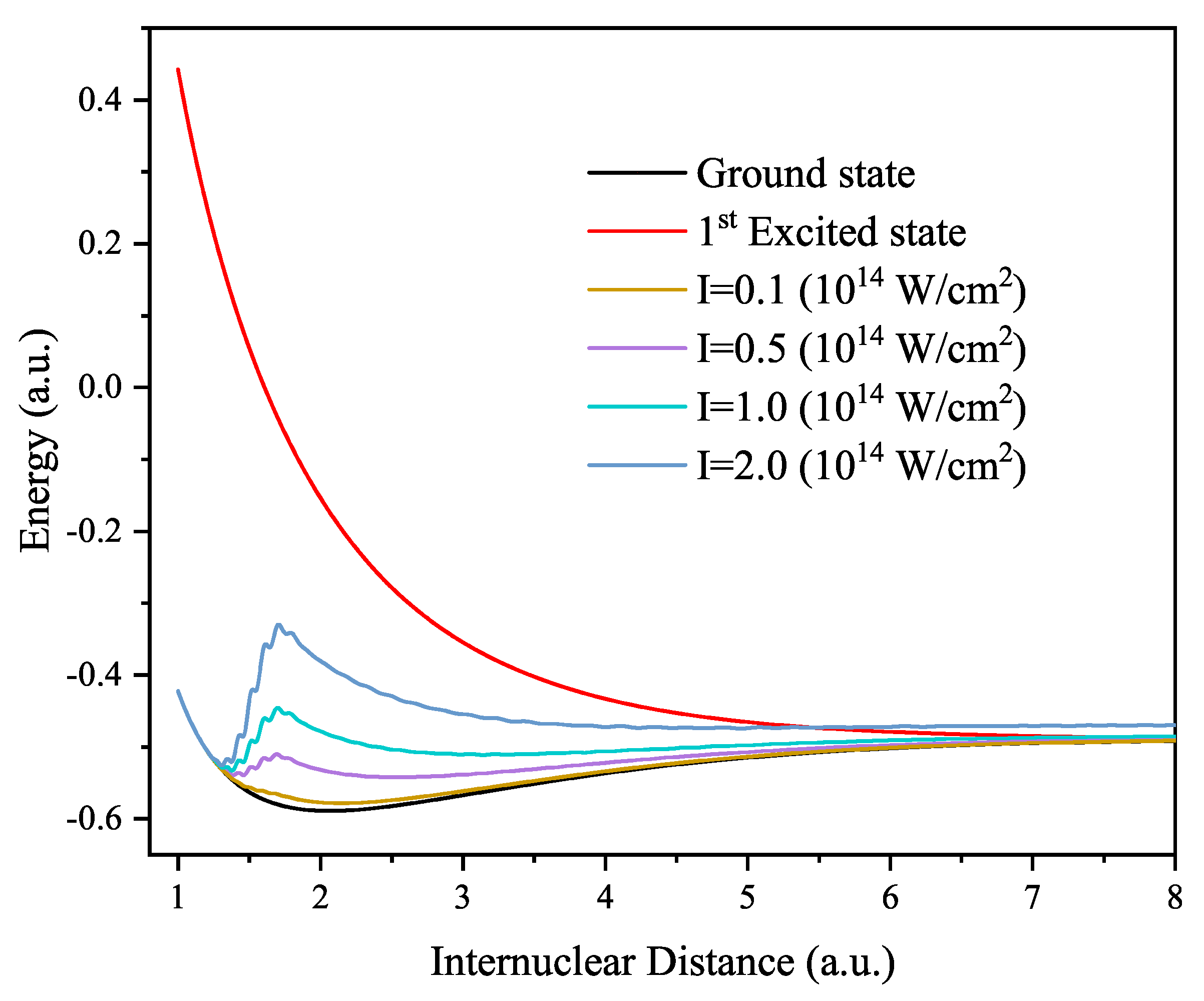
We applied the classical nuclear dynamics approach to achieve the potential energy curves of the ground state and the first excited state of
. At first, we computed the ground state of the system in an initial inter-nuclear distance (
a.u.) by propagating the TDSE in imaginary time over the whole static grid. Then, to compute the first excited state of the system in the same initial inter-nuclear distance, we have employed the Gram-Schmidt algorithm [
32]. Having computed the ground state and the first excited state of the system in an initial inter-nuclear distance, we propagated each of these electronic states in real time in the absence of any external field by considering classical nuclear dynamics. The initial velocity of the two nuclei was set to zero. In this way, the potential energy curves of the ground state and the first excited state of the system were calculated. The simulation results for the dynamic nucleus (DN) approach are plotted in
Figure 1 and compared to the results from the static nucleus (SN) approach [
32] and to the exact values [
39]. It is evident from
Figure 1 that the DN results had a good agreement with the exact values [
39]. In
Figure 1, for the ground state, the computation speed for the short inter-nuclear distances (less than 1.5 a.u.) was high in that the nuclear dynamics at short inter-nuclear distances was fast. As the inter-nuclear distance increased (particularly to greater than 4 a.u.), the nuclear dynamics (and consequently the computation speed) became slower.
For the next round of our investigation, the ground state of
at
a.u. was introduced to a five-cycle ultra-short attosecond laser pulse using a wavelength of
nm and different intensities. Attosecond pulses are needed in such investigations in that the electronic dynamics typically takes place on sub-femtosecond time scales. The shape of such laser pulses for the intensity of
is plotted in
Figure 2. The corresponding energy for a single photon excitation (17.712 eV = 0.6509 a.u.) could be high enough for exciting the ground state of the system to the first excited state at
a.u.
As can be seen from
Figure 3, we tuned our simulation in such a way that when the laser field reached its maximum amplitude, the inter-nuclear distance of
reached
a.u. in the ground state. We repeated the simulation with different laser intensities (from
to
). An interesting phenomenon that could happen at this point is the charge migration between the ground state and the first excited state of the system [
8,
40]. The wave function of the resulting coherent superposition state that corresponds to a spatial displacement of the electronic charge is generally expressed by
In general, the inter-nuclear distance (
) can be varied in time by considering classical nuclear dynamics. It is easy to verify that the time-dependent electron density, which can migrate from one atom to the other, is given by
where
One prerequisite for the occurrence of the charge migration is the existence of spatial overlap (the third term in Equation (
46)) between the electronic wave functions describing the charge in both the ground state and the first excited state [
40]. If we simply consider the initial superposition state in an initial constant inter-nuclear distance as
then we can compute the migration period of electron density from one atom to the other by considering
. By doing so, we obtain
As can be seen from
Figure 4, by employing Equation (
50), we computed the period of charge migration between the two nuclei in
in terms of the inter-nuclear distance. This figure shows that greater inter-nuclear distances corresponded to longer charge migration times between the two nuclei. In
Figure 4, it can be seen that the charge migration period in inter-nuclear distances between 1 and 2 a.u. was relatively low (about 200–300 as) and increased as the inter-nuclear distance grew. From
Figure 4, it can be also conceived that at distances greater than
a.u., the electron density was practically localized on one nucleus.
In order to compute the population of each electronic state
in the coherent superposition state
, implementing the identity operator of CSs (Equation (
11)), one should compute
Applying Equations (
8) and (
9), we reach
From the population results in
Table 1, which were computed (at
a.u.) using Equation (
52), one can deduce that as the intensity of a laser increases, the population of the ground state in the coherent superposition state becomes lower and the population of the excited states becomes higher. In agreement with this deduction, it can be also seen from
Figure 3 that coherent superposition states created by lasers with a lower intensity are closer to the ground state. A higher laser intensity would also lead to a coherent superposition state with more contributors. For example, the coherent superposition state created by using a laser field with an intensity of
(in
Figure 3) had more contributors.
Table 1 and
Figure 3 demonstrate that after exposing the ground state of the system to an attosecond pulse, some of the population was promoted to the excited states. As the intensity of the attosecond laser field was increased, a larger population was transferred to the excited states.
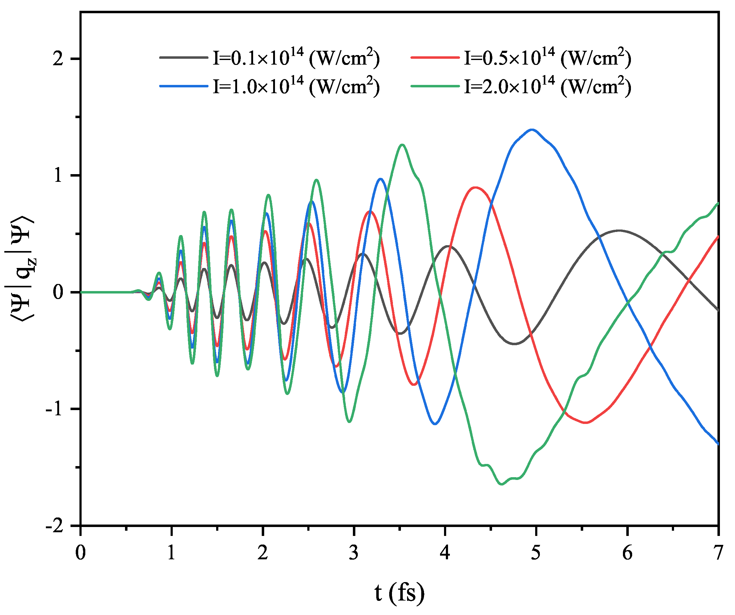
Figure 5 shows the expectation value of the electron coordinate along the
z-axis experiencing ultra-short intense laser pulses with four different intensities. One can see that the amplitude of the coordinate expectation value was larger for higher intensities. However, until 2.0 fs, the period seemed to be the same for all intensities. As the dissociation rate of the two nuclei increased, the period became longer for higher intensities (above
fs). In addition, we calculated the change rate of the inter-nuclear distance for the ground state and the first excited state in the absence of a laser field and for the ground state induced by ultra-short laser pulses with different intensities. The results, depicted in
Figure 6, show that the lowest (highest) rates of dissociation corresponded to the ground (first excited) state in the absence of a laser field.


