Depression Detection Using Relative EEG Power Induced by Emotionally Positive Images and a Conformal Kernel Support Vector Machine

Abstract

Electroencephalography (EEG) can assist with the detection of major depressive disorder (MDD). However, the ability to distinguish adults with MDD from healthy individuals using resting-state EEG features has reached a bottleneck. To address this limitation, we collected EEG data as participants engaged with positive pictures from the International Affective Picture System. Because MDD is associated with blunted positive emotions, we reasoned that this approach would yield highly dissimilar EEG features in healthy versus depressed adults. We extracted three types of relative EEG power features from different frequency bands (delta, theta, alpha, beta, and gamma) during the emotion task and resting state. We also applied a novel classifier, called a conformal kernel support vector machine (CK-SVM), to try to improve the generalization performance of conventional SVMs. We then compared CK-SVM performance with three machine learning classifiers: linear discriminant analysis (LDA), conventional SVM, and quadratic discriminant analysis. The results from the initial analyses using the LDA classifier on 55 participants (24 MDD, 31 healthy controls) showed that the participant-independent classification accuracy obtained by leave-one-participant-out cross-validation (LOPO-CV) was higher for the EEG recorded during the positive emotion induction versus the resting state for all types of relative EEG power. Furthermore, the CK-SVM classifier achieved higher LOPO-CV accuracy than the other classifiers. The best accuracy (83.64%; sensitivity = 87.50%, specificity = 80.65%) was achieved by the CK-SVM, using seven relative power features extracted from seven electrodes. Overall, combining positive emotion induction with the CK-SVM classifier proved useful for detecting MDD on the basis of EEG signals. In the future, this approach might be used to develop a brain–computer interface system to assist with the detection of MDD in the clinic. Importantly, such a system could be implemented with a low-density electrode montage (seven electrodes), highlighting its practical utility.

1. Introduction

Major depressive disorder (MDD) is characterized by persistent sadness, hopelessness, and inability to feel pleasure in normally enjoyable activities (i.e., anhedonia [1]). MDD is also associated with deficits in executive function [2] and memory [3], and recent depression is a risk factor for suicide [4]. Because depression is prevalent and recurrent, the World Health Organization (WHO) ranks it as a leading contributor to the global burden of disease [5]. To effectively treat MDD, a safe, objective, and convenient method for accurate diagnosis is essential. Electroencephalography (EEG) is increasingly recognized as a promising tool in this regard [6], because it is a well-established, inexpensive, and non-invasive method for assessing brain function that is more suitable for routine use than other imaging modalities, such as magnetoencephalography or functional magnetic resonance imaging [7].

Prior studies have used abnormalities in resting-state EEG spectral power to characterize individuals with MDD. Frontal alpha asymmetry [8,9], which refers to relatively greater left versus right alpha band power, is a consistent EEG marker of MDD. Furthermore, the absolute EEG power at specific channels (e.g., alpha power in C3, P3, O1, O2, F7, and T3 [10]) and the average EEG power over channels in specific regions (e.g., frontal alpha and frontal theta [11]) have also been used to distinguish adults with MDD from healthy controls. In short, EEG power may be used to detect MDD. Because MDD is heterogeneous and yields different symptom profiles across patients, the additional information provided by EEG may be very helpful for clinicians seeking to make an accurate diagnosis.

Several studies have, therefore, combined resting-state EEG power features with machine learning to classify individuals as healthy versus depressed. In a study by Hosseinifard et al. [10], classification based on the application of linear discriminant analysis (LDA) to power in the delta, theta, alpha, and beta bands achieved accuracies of 67%, 70%, 73%, and 70%, respectively. Our recent classification study [12] also obtained the best results when applied to alpha power. However, we were only able to achieve a classification accuracy of 68.98% using a k-nearest neighbor (k-NN) classifier. Thus, classification via resting-state EEG spectral power features is characterized by relatively low accuracy. The LDA classification performance results reported in [10,12] could represent the upper limit of classification based on spectral power features, but it is likely that applying a more sophisticated classifier such as a support vector machine (SVM) may improve accuracy. Furthermore, employing an MDD-sensitive task to elicit EEG responses that differ strongly between depressed and healthy individuals may also prove helpful [10,12]. The present study took this approach by applying a novel SVM classifier to EEG data recorded during an emotion induction paradigm completed by adults with MDD and healthy controls.

The task used in the current study focused on the induction of positive emotions. We did not use emotionally negative stimuli, because although excessive negative emotion is a prominent characteristic of MDD, it is also commonly found in anxiety. By contrast, anhedonia—reduced ability to derive pleasure from enjoyable experiences—is relatively specific to depression [13]. Therefore, a blunted neural response to positive stimuli may be more diagnostic of depression versus anxiety. Furthermore, anhedonia has been linked to disruption in brain reward circuitry [14,15,16], and such abnormalities may have consequences for downstream functions, such as episodic memory [17,18,19]. Therefore, abnormal responses to positive stimuli appear to be a reliable and important aspect of depressive illness. To our knowledge, however, no prior study has used positive emotion-induction to improve EEG-based detection of MDD. Based on the literature, we expected that EEG signals recorded from controls and adults with MDD would differ more strongly during exposure to emotionally positive material than at rest.

Therefore, we collected EEG data while healthy controls and adults with MDD attempted to maximize their emotional responses to positive images and during the resting state. Given prior work linking changes in relative power (i.e., the power difference between a pair of electrodes) to shifts in emotional experience [20], we focused the analysis on relative power features from all possible (a) regional inter-hemispheric, (b) cross-regional inter-hemispheric, and (c) intra-hemispheric electrode pairs. We then compared leave-one-participant-out cross-validation (LOPO-CV) classification performance based on EEG relative power features and then determined the best relative power feature subsets for the two states considered separately.

In addition to feature extraction, MDD detector design is also critical to classification performance. Various machine-learning classifiers have been employed in different MDD studies, including the very simple k-NN, LDA, and more sophisticated classifiers like Naïve Bayes (NB), logistic regression (LR), and SVM. Two studies have compared these classifiers for detection of MDD based on EEG signals [10,11]. A comparison of k-NN, LDA, and LR [10] showed that LR achieved the best classification accuracy. More recently, Mumtaz et al. [11] reported that SVM outperformed both LR and NB in MDD-control classification.

Although these results indicate that SVM is the best classifier for EEG-based MDD detection, the classification performance of SVM could still be improved. One strategy for doing so is based on conformal transformation of a kernel proposed by Wu and Amari [21]. The technique of conformally transforming a kernel enlarges the spatial resolution around the SVMs, separating hyperplane in a kernel-induced feature space, thus improving the generalization ability of SVM. This technique has recently been applied to solve problems in other domains, including EEG-based emotion recognition [22]. In the present study, we introduced this variant of SVM, the conformal kernel SVM (CK-SVM), as the MDD detector and compared it with two commonly-used MDD detectors (LDA and SVM) and a variant of LDA classifier called quadratic discriminant analysis (QDA) [23], which has not yet been tested in previous MDD studies. To preview the results, CK-SVM emerged as superior to the other classifiers for EEG-based MDD detection.

2. Materials and Methods

2.1. Participants

Data were collected from 24 adults with MDD (15 females, mean age: 29.7 ± 10.9 y/o, mean education years: 16.3 years) and 31 healthy controls (17 females, mean age: 29.75 ± 9.9 y/o, mean education years: 16.9 years) directly after completion of a source memory task that involved emotionally neutral words [24]. The two groups did not differ in age (p = 0.99), male/female ratio (p = 0.57), or years of education (p = 0.28). The following inclusion criteria were used for the MDD group: (1) endorsed symptoms consistent with a current major depressive episode [25]; (2) a Beck depression inventory II (BDI-II) score ≥13 on the day of the EEG [26]; (3) no other DSM (The Diagnostic and Statistical Manual of Mental Disorders)-IV Axis I psychopathology with the exception of generalized anxiety, social anxiety, and/or specific phobia (all of which are highly comorbid with MDD); and (4) no medication use in the past two weeks (six weeks for fluoxetine, six months for neuroleptics). The controls reported no current or past DSM-IV Axis I psychopathology. As expected, the MDD group generated significantly higher BDI-II scores (mean ± S.D.: 24.96 ± 8.8) than did the controls (1.22 ± 2.01), p <0.001; the BDI-II scores indicate that the participants in the MDD group were moderately depressed, on average. All the participants provided informed consent to a protocol approved by the Partners HealthCare Human Research Committee (PHRC), and they were compensated $25/h for their participation.

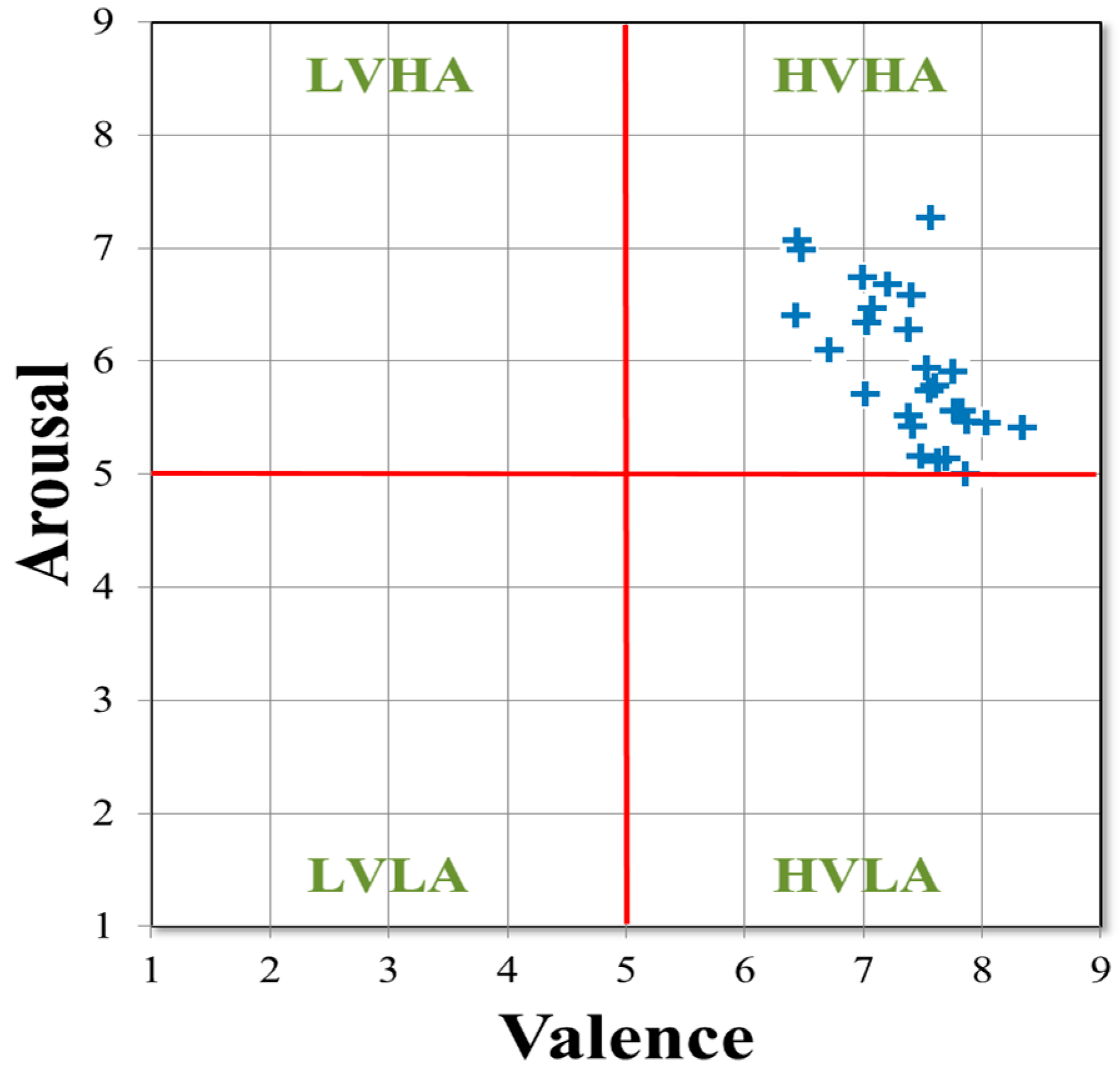
2.2. Emotional Stimuli

Emotionally positive pictures from the International Affective Picture System (IAPS; [27]) were selected based on ratings of valence (ranging from 1 (unpleasant) to 9 (pleasant)) and arousal (ranging from 1 (calm) to 9 (excited)). As shown in Figure 1, the 27 pictures used in this study fall into a “high valence, high arousal” quadrant, as they all possess mean valence and arousal ratings greater than 5 (the mid-point on both scales). The IAPS numbers for the pictures are 2071, 2347, 4607, 8185, 1811, 8420, 8206, 7405, 7330, 8090, 4608, 7230, 8540, 8380, 4660, 4800, 1710, 4626, 8490, 5626, 2345, 7502, 4670, 2045, 5825, 8210, and 8179; we have successfully used this stimulus set in a previous EEG study of emotion recognition [22]. Examples of the pictures are displayed in Figure 2.

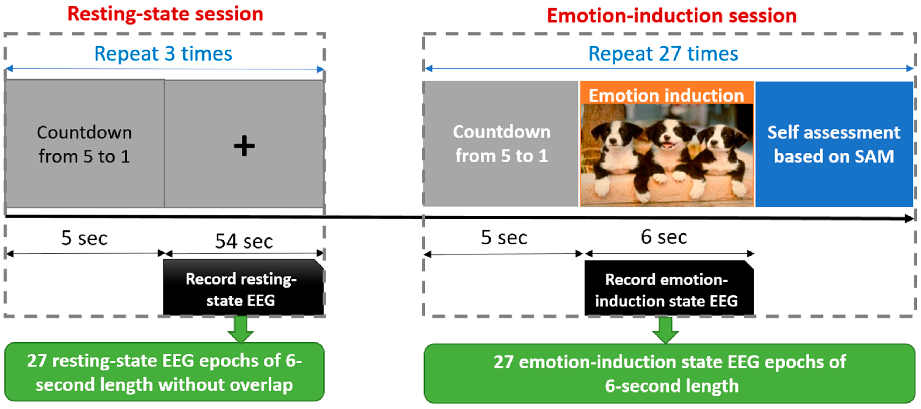
2.3. Resting-State and Emotion-Induction EEG Data Collection

The EEG recording involved a resting-state session followed by the emotion-induction session (Figure 3). All recordings were made in the Center for Depression, Anxiety, and Stress Research at McLean Hospital in Belmont, MA, USA. The resting-state session included three trials. Each trial began with a 5 s countdown, during which time each numeral (5-4-3-2-1) was displayed in black on a gray background for 1 s. This countdown was intended to focus the participants’ attention for the EEG recording. The participants then maintained fixation on a centrally presented black cross displayed on a gray background for 54 s. We recorded 162 s of resting-state data ($54\mathrm{s}/\mathrm{trial}\times 3\mathrm{trials}$), which were subsequently divided into 27 EEG epochs of 6-s length without overlap.

The emotion-induction session included 27 trials. Each trial began with the same 5 s countdown used in the resting-state session. Next, an IAPS picture was shown for a 6-s emotion-induction period. During this period, the participants were asked to engage with the image by imagining that they (or their loved ones) were experiencing the positive event depicted in the picture. Using mental imagery in this way has been shown to effectively enhance and intensify emotional experience in numerous prior studies of emotion regulation, including studies conducted with depressed adults (e.g., [28]). At the end of each trial, the participants used the Self-Assessment Manikin procedure [29] to evaluate the induced emotional experience for valence and arousal. The emotion-induction session was self-paced to avoid fatigue. The participants could take a break whenever they wished, and they initiated each trial by pressing a button. Note that the same amount of raw EEG data (27 epochs of 6-s length) was obtained from each participant during the emotion-induction and resting-state sessions.

2.4. Apparatus, Settings, and EEG Preprocessing

The experimental protocol was programmed with PsychoPy [30], and stimuli were displayed on a 22-inch monitor controlled by a personal computer (PC). The EEG was recorded using a 128-sensor HydroCel GSN Electrical Geodesics Inc. (EGI) Net. The EEG data were referenced to vertex Cz, and impedances were kept below 45 kΩ whenever possible (maximum: 75 kΩ). Eye blinks and movements were monitored by horizontal and vertical bipolar electrooculography (EOG) electrodes. The EEG and EOG data were sampled at 1000 Hz and filtered with a band-pass filter (0.02–100 Hz). The preprocessing of EEG data was performed using EEGLAB toolbox [31]. EEG signals were first band-pass filtered (Finite Impulse Response filter, 0.5~50 Hz, EEGLAB). For the rest of the channels, we performed the independent component analysis (ICA, Infomax, EEGLAB) for the concatenated EEG data and applied the ADJUST algorithm [32] to identify and remove artifact components, including horizontal eye movement, vertical eye movement, eye blinks, and generic discontinuities.

For the purposes of the analysis, we focused on 29 electrodes covering frontal, central, parietal, occipital, and temporal scalp (Figure 4): FP1(22), FP2(9), F3(24), F4(124), Fz(11), F7(33), F8(122), FT7(39), FC3(29), FCz(6), FC4(111), FT8(115), C3(36), C4(104), T3(45), T4(108), CP3(42), CP4(93), CPz(55), TP7(50), TP8(101), P3(52), P4(92), Pz(62), T5(58), T6(96), O1(70), O2(83), and Oz(75). Please note that the number in the parenthesis refers to the original electrode number of the EGI 128-sensors.

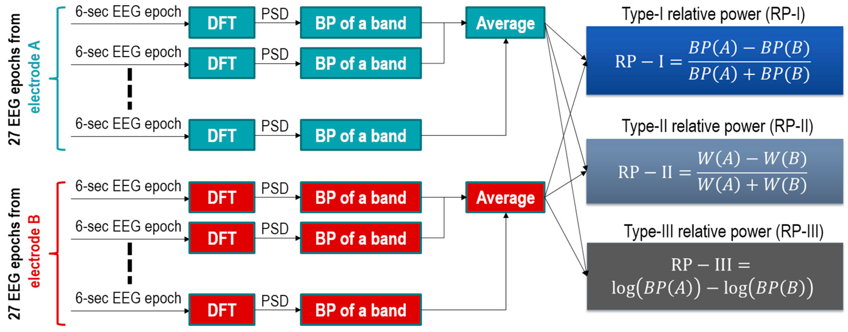
2.5. Feature Extraction

The spectral power density of each electrode’s signal was extracted using discrete Fourier transform (DFT), and the band power (BP) of each frequency band was then calculated. The frequency bands of interest were delta (1–4 Hz), theta (4–8 Hz), alpha (8–13 Hz), beta (13–30 Hz), and gamma (30–45 Hz). For each participant and each electrode, we averaged power in each band across the 27 EEG epochs of the resting and emotion-induction states, separately. For each state and each participant, a total of 29 BP feature values (from 29 electrodes) in each frequency band were obtained. The BPs were subsequently used to calculate relative power features.

Different types of relative powers have been used in various EEG studies. In this study, we extracted the three types of relative power and compared their classification performances (Figure 5). Type-I relative power (RP-I) is calculated with the following formula [33]:

$$\mathrm{RP}-\mathrm{I}=\frac{BP\left(A\right)-BP\left(B\right)}{BP\left(A\right)+BP\left(B\right)}$$

(1)

where $BP\left(A\right)$ and $BP\left(B\right)$ denote the BPs of two different electrodes A and B in the same frequency band. Type-II relative power (RP-II) is given by [11] the following:

$$\mathrm{RP}-\mathrm{II}=\frac{W\left(A\right)-W\left(B\right)}{W\left(A\right)+W\left(B\right)}$$

(2)

where $W$ is the power within a specific band of interest (e.g., alpha) divided by the total power within the entire band of 1–45 Hz. Type-III relative power (RP-III) corresponds to the difference between the natural log-transformed BPs of two different electrodes as follows [8]:

$$\mathrm{RP}-\mathrm{III}=\log \left(BP\left(A\right)\right)-\log \left(BP\left(B\right)\right).$$

(3)

For each frequency band and each type of relative power, a total of 406 ($29\times 28/2$) values were extracted for each participant. These values carry information about regional inter-hemispheric (e.g., FP1-FP2), cross-regional inter-hemispheric (e.g., FP1-T4), and intra-hemispheric (e.g., FP1-O1) asymmetries. Because there are five bands, the number of relative power features of each type (RP-I, RP-II, RP-III) increases to 2030 ($406\times 5$) when all bands are considered. For each kind of feature (e.g., RP-I in a specific frequency band), we obtained one N-dimensional feature vector from each participant. A feature vector is called a data point or a datum in this paper.

2.6. Classification

2.6.1. LDA

The LDA classifier was employed to classify individuals as depressed or healthy. LDA finds a hyperplane as the decision boundary in the original space of patterns. For a test datum $x\in R^N$, where $N$ is the dimension of $x$, the LDA decision function for $x$ is given by the following:

$$D_{LDA}\left(x\right)={\left({\mathsf{\mu }}_1-{\mathsf{\mu }}_2\right)}^T{\mathsf{\Sigma }}^{-1}x-\frac{1}{2}{\left({\mathsf{\mu }}_1-{\mathsf{\mu }}_2\right)}^T{\mathsf{\Sigma }}^{-1}\left({\mathsf{\mu }}_1+{\mathsf{\mu }}_2\right)-\ln \left(\frac{C_{12}{\pi }_2}{C_{21}{\pi }_1}\right)$$

(4)

where ${\mathsf{\mu }}_1$ and ${\mathsf{\mu }}_2$ are the mean vectors of the training data of the first (positive: MDD) and the second (negative: control) classes, respectively, $\mathsf{\Sigma }$ is the $N\times N$ covariance matrix of the training data of the two classes, $C_{12}$ is the penalty weight for the positive class’s training error, $C_{21}$ is the penalty for the negative class’s training error, and ${\pi }_1$ and ${\pi }_2$ are the a priori probabilities of the positive and the negative classes, respectively. Here, we set $C_{12}=C_{21}=1$. The test datum $x$ is classified as MDD if $D_{LDA}\left(x\right)>0$; otherwise, it belongs to the control group.

2.6.2. QDA

The decision function of QDA is given by the following [23]:

$$\begin{gathered} D_{QDA}\left(x\right)=-\frac{1}{2}{x}^T\left({\mathsf{\Sigma }}_1^{-1}-{\mathsf{\Sigma }}_2^{-1}\right)x+\left({\mathsf{\mu }}_1^T{\mathsf{\Sigma }}_1^{-1}-{\mathsf{\mu }}_2^T{\mathsf{\Sigma }}_2^{-1}\right)x-\frac{1}{2}\ln \left(\frac{\left|{\mathsf{\Sigma }}_1\right|}{\left|{\mathsf{\Sigma }}_2\right|}\right) \\ -\frac{1}{2}\left({\mathsf{\mu }}_1^T{\mathsf{\Sigma }}_1^{-1}{\mathsf{\mu }}_1-{\mathsf{\mu }}_2^T{\mathsf{\Sigma }}_2^{-1}{\mathsf{\mu }}_2\right)-\ln \left(\frac{C_{12}{\pi }_2}{C_{21}{\pi }_1}\right) \end{gathered}$$

(5)

where ${\mathsf{\Sigma }}_1$ and ${\mathsf{\Sigma }}_2$ are the covariance matrices of class 1 and class 2, respectively, and $\mathsf{\Sigma }={\pi }_1{\mathsf{\Sigma }}_1+{\pi }_2{\mathsf{\Sigma }}_2$. If $D_{QDA}\left(x\right)>0$, $x\in \mathrm{class}1$; otherwise, $x\in \mathrm{class}2$. Both LDA and QDA have the parameters and $C_{12}$ and $C_{21}$. For a fair comparison, we set $C_{12}=C_{21}=1$.

2.6.3. SVM

Given a training set $S={\left\{\left(x_{i, }{y}_i\right)\right\}}_{i=1}^L$, where $L$ is the size of the set $S$ and $y_i\in \left[-1, +1\right]$ are class labels of the training datum $x_{i, }$, SVM maps the training set into a higher-dimensional feature space F via a nonlinear mapping $\phi$ and then finds a separating hyperplane $w^T\phi \left(x\right)+b=0$ ($H=0$) that minimizes the training error and maximizes the margin of separation between classes. For a test datum $x$, its output can be estimated by the SVM decision function as follows:

$$D_{SVM}\left(x\right)={\displaystyle \sum }_{x_{i }\in SV}{\alpha }_i{y}_{i}k\left(x_{i, },x\right)+b_{opt}$$

(6)

where $0\le {\alpha }_i\le C$ are Lagrange multipliers, $C$ is the penalty weight for training error, SV denotes the set of support vectors: $SV=\left\{x_i|0<{\alpha }_i\le C\right\}, b_{opt}$ is the optimum bias of the separating hyperplane (determined according to the Kuhn–Tucker condition of SVM), and $k(,)$ is the kernel function, which computes the inner product of two mapped data in the space F. In this study, the Gaussian function $k\left(x_{i, },x\right)=exp(\Vert x_i-x{\Vert }^2/2{\sigma }^2)$ was adopted as the kernel of SVM, where $\sigma$ is the parameter of the kernel. The test datum $x$ is classified as MDD if $D_{SVM}\left(x\right)>0$; otherwise, $x$ is classified as the control group.

2.6.4. CK-SVM

The Gaussian kernel embeds the original space $R^N$ into an infinite dimensional space F as a Riemannian manifold lying on a unit ball centered at the origin of the space F (see the author’s previous work [34] for an illustration), and the kernel-induced Riemannian metric is given by the following:

$$g_{ij}\left(x\right)={\frac{\partial k\left(x,x^{\prime }\right)}{\partial x_i\partial x_j^{\prime }}|}_{x^{\prime }=x}$$

(7)

where x_i denotes the ith element of $x$. The relationship between the Riemannian distance $ds$ and a small displacement $dx$, as follows,

$$d{s}^2={\displaystyle \sum }_{i,j}{g}_{ij}\left(x\right)d{x}_{i}d{x}_j$$

(8)

indicates how a local volume in $R^N$ is magnified or contracted in F under the mapping of $\phi$. A conformal transformation of $\phi$ is defined by $\tilde{\phi }\left(x\right)=Q\left(x\right)\phi \left(x\right)$, where $Q\left(x\right)$ is a real-valued conformal function. The function $Q\left(x\right)$ can be chosen in a way in which its value is the largest at the vicinity of $\phi \left(x\right)$ and decreases with the distance from the position of $\phi \left(x\right)$. Designing such a transformation yields the conformal transformation of a primary kernel $k$ as follows:

$$\tilde{k}\left(x,x^{\prime }\right)=Q\left(x\right)Q\left(x^{\prime }\right)k\left(x,x^{\prime }\right)$$

(9)

where the transformed kernel $\tilde{k}$ is called a conformal kernel. Let a set T contain a set of data points $x_{\mathit{i}}s$. To magnify the spatial resolution around the images of the data points $x_{\mathit{i}}s$ in the space F, a conformal function consisting of a set of Gaussian functions can be defined as follows [21]:

$$Q\left(x\right)={\displaystyle \sum }_{x_{\mathit{i}}\in \mathit{T}}exp\left(\frac{\Vert \phi \left(x\right)-\phi \left(x_{\mathit{i}}\right){\Vert }^2}{\frac{1}{n}{{\displaystyle \sum }}_{\mathit{j}}\Vert \phi \left(x_{\mathit{j}}\right)-\phi \left(x_{\mathit{i}}\right){\Vert }^2}\right)$$

(10)

where the denominator term $\frac{1}{n}{\displaystyle \sum }_{\mathit{j}}\Vert \phi \left(x_{\mathit{j}}\right)-\phi \left(x_{\mathit{i}}\right){\Vert }^2$ computes the mean squared distance from the image of $x_{\mathit{i}}$ to its n nearest neighbors $\phi \left(x_{\mathit{j}}\right)$. According to Equation (9), the conformal function $Q\left(x\right)$ has the largest value at the position of the image of the set T and decays with the distance from the image of T in the feature space F. Wu and Amari [21] proposed that the set T should collect the training data points whose ${\alpha }_i>0$ (i.e., the support vectors) based on the fact that most support vectors lie within the margin of separation. However, some support vectors may be far from the margin. Accordingly, Liu et al. [22] defined the set T as follows:

$$T=\left\{x_{\mathit{i}}|x_{\mathit{i}}\in SV and \left|D_{SVM}\left(x_i\right)\right|\le 1\right\}.$$

(11)

Because the training data points in the set T are the support vectors falling inside of the separation margin, enlarging the spatial resolution around the image of the set T, defined as Equation (11), is equivalent to increasing the spatial resolution of the separation margin in the feature space F. In this paper, we adopted the conformal function and the set T suggested in [21,22], respectively. Because the Gaussian function is adopted as the kernel, $k\left(x,y\right)=1, \forall x=y$. Thus, the conformal function expressed in Equation (10) can be simplified as follows:

$$Q\left(x\right)={{\displaystyle \sum }}_{x_{\mathit{i}}\in \mathit{T}}exp\left(\frac{2-2k\left(x,x_{\mathit{i}}\right)}{\frac{1}{n}{{\displaystyle \sum }}_{\mathit{j}}\left(2-2k\left(x_{\mathit{j}},x_{\mathit{i}}\right)\right)}\right).$$

(12)

In this study, we set $n=3$. The training of CK-SVM consists of two steps: firstly, train an SVM with a Gaussian kernel; and secondly, retrain the SVM with the conformal kernel defined in Equation (9).

2.7. Performance Evaluation

2.7.1. LOPO-CV

In the present study, we performed leave-one-participant-out cross-validation (LOPO-CV) to assess the participant-independent MDD-control classification performance for each combination of feature, classifier, and session (resting and emotion-induction). LOPO-CV is a technique for evaluating how well the results of a method will generalize to unseen data. In each fold of the LOPO-CV, data from 54 participants were used to train the classifier, and then, the N-dimensional data from the one remaining participant were used as the test data. This step was repeated until every participant’s data had served as the test data once. We then recorded the classification accuracy, computed as the number of correctly classified participants divided by the total number of participants (55 folds). Here, a misclassified datum in a testing fold resulted in only a small increase of error rate (1/55 = 1.82%).

2.7.2. Parameter Optimization

None of the three types of relative power feature extraction methods used free parameters. As for the classifiers, LDA involves no free parameters, and both SVM and CK-SVM have two parameters to be adjusted, including the penalty weight $C$ and kernel parameter $\sigma$. We searched for the optimum parameters by performing the LOPO-CV procedure combined with a grid search. The parameters were searched in the following sets: $C=\left\{1, 10, 20, 50, 80, 100, 120\right\}$, $\sigma =\left\{{1.025}^d\right|d=-100:1:300\}$. Therefore, there was a total of 2807 ($7\times 401$) parameter grids, and for each grid, the LOPO-CV procedure was performed once. The optimum parameter grid resulted in the highest classification accuracy. The results of SVM and CK-SVM reported here were the ones obtained from the most optimal values of the parameters.

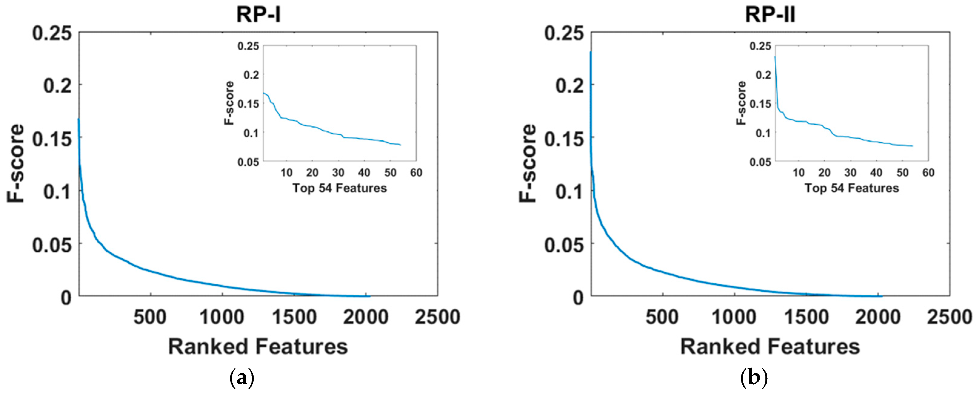
2.7.3. Feature Dimension Reduction

Directly including all the features in the LOPO-CV procedure might result in overfitting. Take RP-I of the delta band as an example. A total of 406 delta-band PR-I features were extracted from each participant. If we were to include all the features in the classification, the feature dimension would be 406 ($N=406$). This is obviously higher than the size of the training set ($\left|S\right|=54$) in each fold of the LOPO-CV, leading to the so-called small sample size (SSS) problem. The SSS problem may have two critical consequences. First, it may lead to overfitting [35]. Second, the covariance matrix of LDA may become singular such that its inverse does not exist [22]. Although it is possible to calculate the pseudoinverse of the covariance in such cases, classification performance would nevertheless degenerate. To avoid the SSS problem, feature selection must be used to reduce the feature dimension to 54 prior to LOPO-CV.

Feature selection methods can be classified into three categories: embedded, wrapper, and filter [36]. Embedded and wrapper methods rely on the performance of a specific classifier to quantify the classification ability of each feature. Examples of the former and the latter are sequential forward selection (SFS) [37] and recursive feature elimination (RFE) methods [38], respectively. By contrast, filter methods are independent of the classifier. One popular filter method is Fisher’s class separability criterion [39]. This involves calculating the Fisher ratio (F-score) for each feature, and then ranking the features by their F-scores. A higher F-score corresponds to a higher between-class to within-class ratio for the feature. By contrast, a lower F-score indicates that the feature is noisier. The advantage of the filter method is its low computational complexity. Therefore, for each state and each type of RPs, we applied Fisher’s method to select the top 54 features from the 406 single-band (delta/theta/alpha/beta/gamma) and the 2030 “all-band” RP feature candidates, respectively. Note that the objective was not to select a set of “optimum features”, but simply to select 54 features to avoid the small sample size problem. Figure 6 shows the F-scores of the 2030 (all bands) RP-I, RP-II, and RP-III features extracted during the emotion-induction state.

The next question is how to find the most useful features among a given set of F-score ranked features. To address this issue, Lin et al. [20] conducted two experiments based on a leave-N-feature-out scheme to select the best EEG features from 60 candidates. Their first experiment iteratively removed N F-score-ranked features one at a time and examined each one’s effects on classification performance. In the second experiment, they iteratively removed N F-score-ranked features one at a time, but the removed N features were randomly selected. Their results based on different N values (e.g., 1, 5, 10, 15, and 20) showed that the top F-score-ranked features were more discriminative than the lower ranked ones. As a result, they suggested that one may directly choose the top-N features as the optimum feature subset for emotional EEG classification, and the optimal value of N can be determined by a data driven method (i.e., cross-validation). Recently, the same strategy for selecting the top-N-F-score-ranked features was adopted for classifying motor imagery EEG [40].

Accordingly, in this study, we performed LOPO-CV to calculate the classification accuracy using the top-N-F-score-ranked features for each state (resting and emotion induction) and each RP type, and this procedure was conducted once for every N ($N=1,2,\dots ,54$). Here, we used the LDA as the classifier, because a sophisticated classifier such as a nonlinear SVM classifier may compensate for the weakness of a feature, and thus, a simple classifier is preferred in feature evaluation [41]. Also, LDA involves no free parameters, and thus, there is no need to perform the time-consuming grid search method for each N.

2.8. Statistical Analysis

In the current study, we used the Wilcoxon rank-sum test to test for a group difference (MDD vs control) in the subjective ratings of valence and arousal elicited by the IAPS pictures.

3. Results

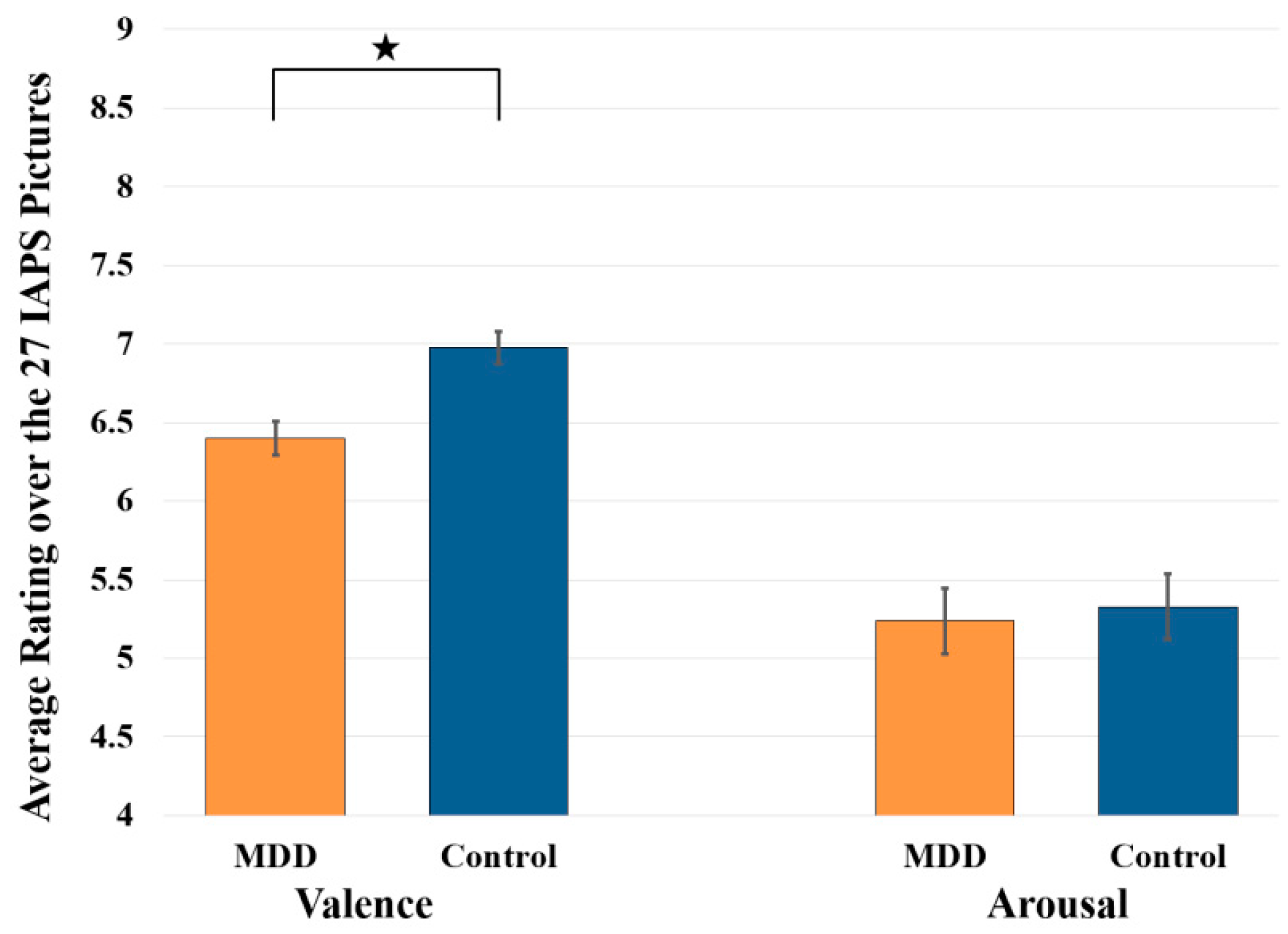
3.1. Statistical Analysis Results of Subjective Ratings of Valence and Arousal

Figure 7 shows that the average valence of the emotional responses elicited by the pleasant pictures was significantly lower (p < 0.0005) in the MDD group (6.40 ± 0.11) versus the healthy control group (6.98 ± 0.10). By contrast, there was no difference in arousal ratings (MDD: 5.24 ± 0.21; Control: 5.33 ± 0.21, p = 0.79). Thus, MDD selectively blunted the pleasantness—but not the overall arousal—of the emotional responses elicited by the positive pictures.

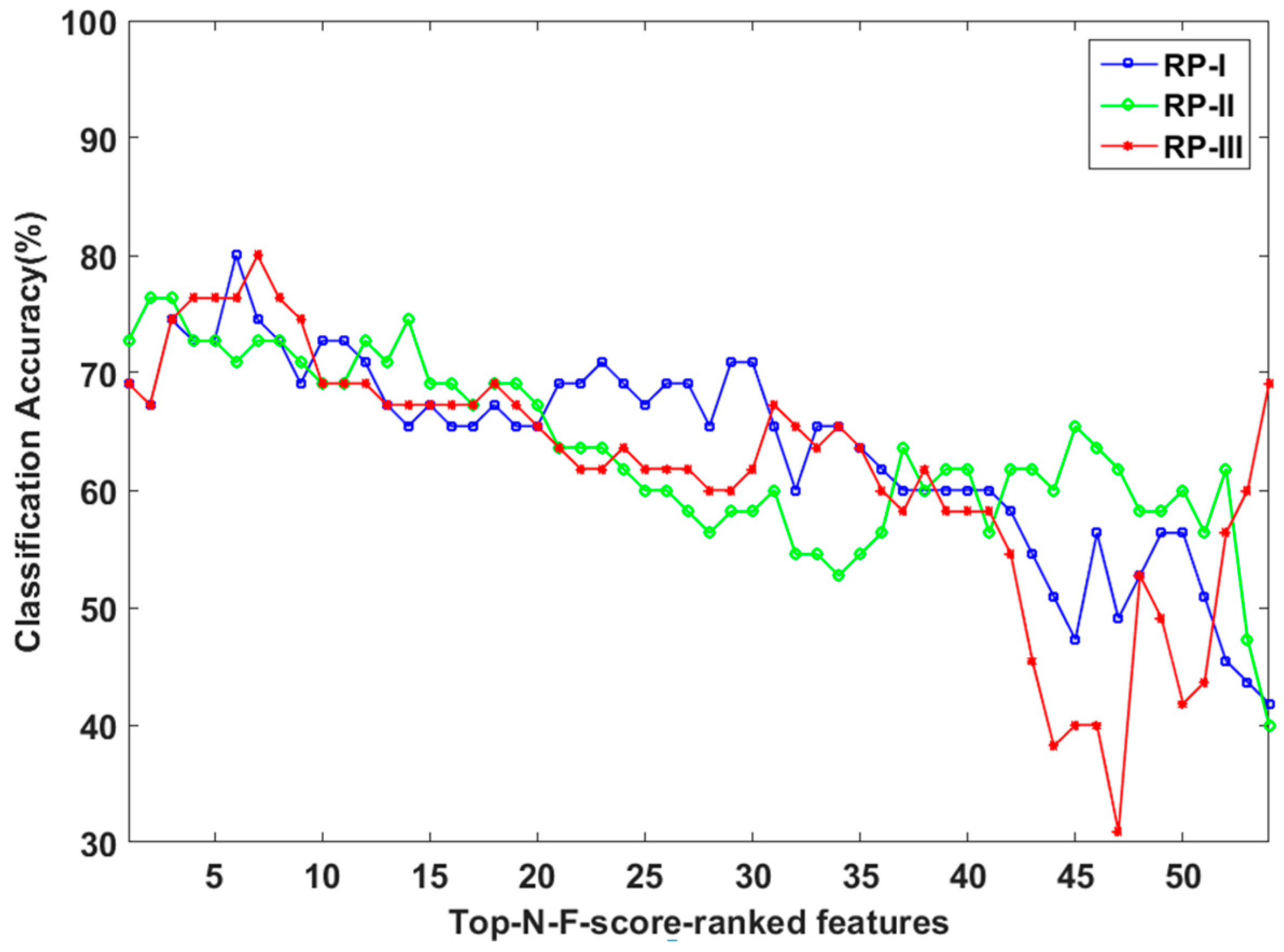
3.2. LOPO-CV Classification Results Based on LDA Classifier and Top-N-F-Score-Ranked Features

Figure 8 shows the classification accuracy obtained by each top-N-F-score-ranked feature set in different types of RP extracted from the emotion-induction state. Figure 6 shows that overall, the three accuracy curves decrease with the increase of N. The highest classification accuracies for the three types of RPs are 80.00% (N = 6), 76.36% (N = 2), and 80.00% (N = 7), respectively. The best numbers of the top-N-F-score-ranked features (i.e., the best N) for different types of RPs were apparently different.

Table 1. A comparison of linear discriminant analysis (LDA)-based leave-one-participant-out cross-validation (LOPO-CV) classification accuracy between the resting and the emotion-induction (EI) states in different conditions of frequency bands. The number in the parenthesis refers to the best number of N.

Feature	State	Delta Band	Theta Band	ALPHA Band	Beta Band	Gamma Band	All Bands
RP-I	Resting	65.45% (2)	70.91% (7)	63.64% (1)	65.45% (44)	61.82% (3)	74.55% (7)
	EI	72.73% (2)	74.55% (2)	72.73% (31)	78.18% (45)	74.55% (2)	80.00% (6)
RP-II	Resting	65.45% (53)	70.91% (24)	61.82% (3)	63.64% (32)	67.27% (3)	70.91% (3)
	EI	76.36% (13)	76.36% (35)	74.55% (4)	70.91% (19)	72.73% (2)	76.36% (2)
RP-III	Resting	65.45% (2)	69.09% (5)	63.64% (1)	67.27% (39)	65.45% (35)	74.55% (7)
	EI	78.18% (2)	74.55% (2)	65.45% (3)	69.09% (2)	70.91% (2)	80.00% (7)

further compares the MDD-control classification accuracy between the best N features extracted from the resting state and the emotion-induction state in different conditions of frequency bands.

As shown in Table 1, the classification accuracy is higher than 70% in the “all bands” condition for RP-I (74.55%), RP-II (70.91%), and RP-III (74.55%). When the classification was based on the emotion-induction state, the classification accuracy improved to 80.00%, 76.36%, and 80.00%, respectively. In fact, emotion-induction outperformed the resting state for every combination of RP type and frequency. To quantify how much classification accuracy improved for the emotion-induction state versus the resting state, we computed the accuracy improvement ratio (AIR), defined as follows:

$$\mathrm{AIR}=\frac{accuracy \left(EI\right)-accuracy\left(resting\right)}{accuracy\left(resting\right)}\times 100\%$$

(13)

As shown in Figure 9, the AIRs were all positive. This reveals a consistent advantage for classification based on EEG data from the emotion-induction session versus the resting state. The results in Table 1 and Figure 9 demonstrate that, compared with the resting state, the emotion-induction state induces EEG signals that differ more sharply across depressed versus healthy adults.

Table 1 further highlights that, for each type of RP and each recording state, the accuracy of the “all bands” condition is higher than that for any single band. Take the resting-state RP-I as an example. The accuracies of the five single bands (delta, theta, alpha, beta, and gamma) are 65.45%, 70.91%, 63.64%, 65.45%, and 61.82%, respectively, which are all lower than that in the “all bands” condition (74.55%). This observation indicates that using all the data from different frequency bands results in better accuracy than using the data from any single frequency.

3.3. Comparison of Top-N-F-Score-Ranked Features Across the Three Types of Relative Power During Resting State and Emotion-Induction State

Table 2. Best top-N-F-score-ranked relative power features in the “all-band” condition.

	Resting State			Emotion Induction
Ranking	RP-I	RP-II	RP-III	RP-I	RP-II	RP-III
1	FP1-FP2(α)	T4-CP4(γ)	FP1-FP2(α)	FP1-FP2(δ)	FP1-FP2(α)	FP1-FP2(δ)
2	Fz-FCz(θ)	F8-C4(γ)	Fz-FCz(θ)	FP1-FP2(θ)	TP7-T6(β)	FP1-FP2(θ)
3	T4-CP4(γ)	FC3-CP3(θ)	FP1-FP2(θ)	TP7-T6(β)		TP7-T6(β)
4	FT8-CP4(γ)		FT8-T4(δ)	C3-TP7(γ)		F4-CP3(θ)
5	FP1-FP2(θ)		CP3-CP4(γ)	C3-CP3(γ)		C3-CP3(γ)
6	FT8-T4(δ)		FT8-CP4(γ)	F4-CP3(θ)		F4-CP3(α)
7	F8-C4(γ)		FT8-T4(θ)			TP7-T6(γ)
# electrodes	9	6	9	7	4	7

lists the best top-N features in each state and in each RP condition. Note that for each type of RP, there is almost no overlap between the best feature sets from the resting state and emotion-induction state. For both RP-I and RP-III, there is only one common relative power feature (i.e., frontal theta asymmetry: theta band FP1-FP2) for the resting and the emotion-induction states. As for RP-II, there is no overlap between the two states. Thus, the brain activity that distinguishes the participants with MDD from the healthy controls is different during rest versus positive emotion induction. Of particular interest, one notable difference is the shift from frontal alpha asymmetry at rest to frontal delta asymmetry during positive emotion induction. As shown in Table 2, for both RP-I and RP-III, the top features were FP1-FP2(α) in the resting state, but this became FP1-FP2(δ) during the positive emotion induction.

3.4. Comparison of LOPO-CV Classification Performance Among Different Classifiers in the-Emotion Induction State

Table 3. Comparison of accuracy for different classifiers using data from the emotion-induction state. QDA = quadratic discriminant analysis; and CK-VSM = conformal kernel support vector machine.

Feature	LDA	QDA	SVM	CK-SVM
RP-I (6)	80.00%	65.45%	81.82%	81.82%
RP-II (2)	76.36%	74.55%	78.18%	80.00%
RP-III (7)	80.00%	70.91%	80.00%	83.64%

lists the best emotion-induction LOPO-CV classification accuracies, where the relative power features of each type are the best ones listed in Table 2. Among the four classifiers, QDA performed the worst for all types of RP features, and CK-SVM performed the best in RP-II and RP-III. When the best features of RP-I were used, SVM and CK-SVM achieved identical accuracy. The results indicate that, overall, CK-SVM outperformed SVM. Finally, the combination of RP-III features and the CK-SVM classifier achieved the highest accuracy of 83.64%. This corresponds to the correct classification of 46 of the 55 participants: 21 of the 24 MDD participants were detected (sensitivity = 87.50%), and 25 of the 31 healthy controls were correctly classified (specificity = 80.65%).

4. Discussion

It was easier to classify adults as depressed versus healthy using EEGs recorded during a positive emotion-induction state as compared with the resting state. This may reflect the altered response to positive emotional stimuli and rewarding experiences previously reported in depressed adults [14,15,16,18]. Along these lines, our behavioral data revealed that MDD blunted the pleasantness—but not the overall arousal—of the emotional responses to positive pictures. Future studies may wish to investigate correlations between the extent of positive emotional dysregulation in depressed adults and classification accuracy based on EEG data collected during emotion induction.

Although the current study used IAPS pictures to induce emotional responses, it is important to note that this is not the only publicly available database of emotional stimuli. Other public resources such as the International Affective Digitized Sounds (IADS) and the Database for Emotion Analysis using Physiological signals (DEAP) have also been used in recent EEG studies [42,43]. Both IADS and DEAP include stimuli with positive emotional content. It is unclear whether the findings in the current study—especially the promising classification performance of those best relative power features—would generalize to emotion induction using positive stimuli selected from IADS or DEAP. Because the cortical activities that underlie emotional responses may vary somewhat with the sensory nature of the eliciting stimulus (e.g., multisensory stimuli in DEAP vs visual stimuli in IAPS), it will be important to address this issue in future work. Furthermore, emotional responses are known to vary across cultures [44,45]. Because all participants in the present study came from the United States (US), future studies should address whether the current findings apply to different settings.

The findings of this study have several implications for developing an EEG-based brain-computer interface (BCI) system for the detection of MDD. First, the extraction of the top seven F-score-ranked RP-III features induced by the positive emotional stimuli required only seven EEG recording sites, including FP1, FP2, TP7, T6, F4, CP3, and C3 (Table 2). If these results can be replicated, the implication is that a low-density electrode montage could be used to obtain similar classification accuracies. A low-density montage can be setup quickly if a dry-electrode or non-gel-based electrode system is used (e.g., the EGI system used in this study). Even if a gel-based recording system is applied (e.g., the NuAmp made by NeuroScan Inc.), the preparation stage (including applying electric gel to reduce the impendence of the seven electrodes) could be accomplished in about 10 min by experienced users, which would make clinical application of the BCI system feasible.

Second, the current study showed that the combination of positive emotion-induction RP-III features and a CK-SVM classifier yielded the highest classification accuracy. Therefore, this combination could provide clinicians with a useful tool for assisting with the detection of MDD. Obviously, the results of this study must be replicated before considering a transition to clinical settings. Moreover, it may be possible to improve classification performance further by using other types of EEG features that have been proven useful for distinguishing between healthy and depressed individuals in prior studies, such as nonlinear features based on fractal dimension (FD) analysis (e.g., Higuchi’s FD [6], correlation dimension [10], Katz’ FD [46]), and the spectral–spatial features based on kernel eigen-filter-bank common spatial pattern (KEFB-CSP) proposed in our recent work [12]. All these features may also perform better in the positive emotion-induction state than in the resting state. Although discussion of these other features is beyond the scope of the current study, they certainly merit attention in future work.

Finally, the clinical implications of this work deserve consideration. The diagnosis of MDD is currently assigned based on diagnostic interviews and self-reports. This is problematic, because individuals typically underreport their depressive symptoms [47]. This is especially true for men relative to women [48,49] and for individuals from Asian as opposed to Western cultures [50,51]. Consequently, MDD is often underdiagnosed in such participants, which results in needless suffering. This important issue could be resolved by application of the EEG-based method described here, because it does not rely on self-reporting for detecting depression. For this possibility to materialize, however, the method will need to be validated in such participants.

If this idea is pursued further, it would be valuable to simultaneously try to identify EEG signals that can predict which individuals will respond to which specific treatment. Matching treatments to patients is currently based on a trial-and-error approach that is inefficient: many individuals must cycle through several treatments before finding one that works for them. To combat this problem, recent studies have identified specific variables—measured behaviorally or via self-reports—that can be used to identify the optimal treatment for individuals on the first try [52,53]. MDD, however, is a heterogeneous disorder that likely involves multiple distinct pathophysiologies. These pathophysiologies may be difficult to tease apart behaviorally or by self-reporting, but they may respond very differently to various treatments. Because EEG is a direct measure of brain activity, it is presumably closer to the pathophysiological process, and so, it may be possible to identify EEG-based signals that could be used for treatment prediction (e.g., [54]). In short, an important next step will be to use EEG signals not only to distinguish between individuals with MDD and healthy controls, but to identify the particular intervention that is likely to work best for one depressed participant versus another.

5. Conclusions

The current study investigated the value of positive emotion induction as a method for eliciting EEG signals that could aid in the classification of adults as healthy versus depressed. It also compared three types of relative power features (RP-I, RP-II, and RP-III) that have been adopted in different MDD studies and introduced a variant of SVM—the CK-SVM—as an MDD detector. There are three main findings. First, for all types of RPs, the best F-score-ranked features in the resting state and the emotion-induction state were quite different. Second, for all types of RPs, LOPO-CV classification accuracy was better for EEG collected during the positive emotion-induction versus the resting state. Finally, the CK-SVM classifier outperformed the other three classifiers, yielding an accuracy of 83.64% in the use of the RP-III feature. All the three findings were based on the cross-validation results. In the future, it will be necessary to test these methods (positive emotion-induction EEG relative powers and the CK-SVM classifier) on an independent dataset. In the meantime, the application of the CK-SVM classifier to EEG data collected during a positive emotion-induction state is a promising method for classifying adults as healthy or depressed.

References

1. American Psychiatric Association. Diagnostic and Statistical Manual of Mental Disorders: DSM-5, 5th ed.; DSM-5 Task Force; American Psychiatric Association: Washington, DC, USA, 2013; p. xliv. 947p. [Google Scholar]
2. Snyder, H.R. Major depressive disorder is associated with broad impairments on neuropsychological measures of executive function: A meta-analysis and review. Psychol. Bull. 2013, 139, 81–132. [Google Scholar] [CrossRef] [PubMed]
3. Burt, D.B.; Zembar, M.J.; Niederehe, G. Depression and memory impairment: A meta-analysis of the association, its pattern, and specificity. Psychol. Bull. 1995, 117, 285–305. [Google Scholar] [CrossRef] [PubMed]
4. Nock, M.K.; Dempsey, C.L.; Aliaga, P.A.; Brent, D.A.; Heeringa, S.G.; Kessler, R.C.; Stein, M.B.; Ursano, R.J.; Benedek, D. Psychological autopsy study comparing suicide decedents, suicide ideators, and propensity score matched controls: Results from the study to assess risk and resilience in service members (Army STARRS). Psychol. Med. 2017, 47, 2663–2674. [Google Scholar] [CrossRef] [PubMed]
5. Vos, T.; Flaxman, A.D.; Naghavi, M.; Lozano, R.; Michaud, C.; Ezzati, M.; Shibuya, K.; Salomon, J.A.; Abdalla, S.; Aboyans, V.; et al. Years lived with disability (YLDs) for 1160 sequelae of 289 diseases and injuries 1990–2010: A systematic analysis for the global burden of disease study 2010. Lancet 2012, 380, 2163–2196. [Google Scholar] [CrossRef]
6. Mumtaz, W.; Malik, A.S.; Yasin, M.A.M.; Xia, L.K. Review on EEG and ERP predictive biomarkers for major depressive disorder. Biomed. Signal Process. Control 2015, 22, 85–98. [Google Scholar] [CrossRef]
7. Liu, Y.H.; Wang, S.H.; Hu, M.R. A self-paced P300 healthcare brain-computer interface system with SSVEP-based switching control and kernel FDA plus SVM-based detector. Appl. Sci. 2016, 6, 142. [Google Scholar] [CrossRef]
8. Segrave, R.A.; Cooper, N.R.; Thomson, R.H.; Croft, R.J.; Sheppard, D.M.; Fitzgerald, P.B. Individualized alpha activity and frontal asymmetry in major depression. Clin. EEG Neurosci. 2011, 42, 45–52. [Google Scholar] [CrossRef] [PubMed]
9. Tas, C.; Cebi, M.; Tan, O.; Hizli-Sayar, G.; Tarhan, N.; Brown, E.C. EEG power, cordance and coherence differences between unipolar and bipolar depression. J. Affect. Disord. 2015, 172, 184–190. [Google Scholar] [CrossRef] [PubMed]
10. Hosseinifard, B.; Moradi, M.H.; Rostami, R. Classifying depression patients and normal subjects using machine learning techniques and nonlinear features from EEG signal. Comput. Methods Programs Biomed. 2013, 109, 339–345. [Google Scholar] [CrossRef] [PubMed]
11. Mumtaz, W.; Xia, L.K.; Ali, S.S.A.; Yasin, M.A.M.; Hussain, M.; Malik, A.S. Electroencephalogram (EEG)-based computer-aided technique to diagnose major depressive disorder (MDD). Biomed. Signal Process. Control 2017, 31, 108–115. [Google Scholar] [CrossRef]
12. Liao, S.C.; Wu, C.T.; Huang, H.C.; Cheng, W.T.; Liu, Y.H. Major depression detection from EEG signals using kernel eigen-filter-bank common spatial patterns. Sensors 2017, 17, 1385. [Google Scholar] [CrossRef] [PubMed]
13. Watson, D.; Weber, K.; Assenheimer, J.S.; Clark, L.A.; Strauss, M.E.; McCormick, R.A. Testing a tripartite model: I. Evaluating the convergent and discriminant validity of anxiety and depression symptom scales. J. Abnorm. Psychol. 1995, 104, 3–14. [Google Scholar] [CrossRef] [PubMed]
14. Pizzagalli, D.A. Depression, stress, and anhedonia: Toward a synthesis and integrated model. Annu. Rev. Clin. Psychol. 2014, 10, 393–423. [Google Scholar] [CrossRef] [PubMed]
15. Proudfit, G.H. The reward positivity: From basic research on reward to a biomarker for depression. Psychophysiology 2015, 52, 449–459. [Google Scholar] [CrossRef] [PubMed]
16. Treadway, M.T.; Zald, D.H. Reconsidering anhedonia in depression: Lessons from translational neuroscience. Neurosci. Biobehav. Rev. 2011, 35, 537–555. [Google Scholar] [CrossRef] [PubMed] [Green Version]
17. Dillon, D.G. The neuroscience of positive memory deficits in depression. Front. Psychol. 2015, 6, 1295. [Google Scholar] [CrossRef] [PubMed]
18. Dillon, D.G.; Dobbins, I.G.; Pizzagalli, D.A. Weak reward source memory in depression reflects blunted activation of VTA/SN and parahippocampus. Soc. Cognit. Affect. Neurosci. 2014, 9, 1576–1583. [Google Scholar] [CrossRef] [PubMed]
19. Dillon, D.G.; Pizzagalli, D.A. Mechanisms of memory disruption in depression. Trends Neurosci. 2018, 41, 137–149. [Google Scholar] [CrossRef] [PubMed]
20. Lin, Y.P.; Wang, C.H.; Jung, T.P.; Wu, T.L.; Jeng, S.K.; Duann, J.R.; Chen, J.H. EEG-based emotion recognition in music listening. IEEE Trans. Biomed. Eng. 2010, 57, 1798–1806. [Google Scholar] [PubMed]
21. Wu, S.; Amari, S. Conformal transformation of kernel functions: A data-dependent way to improve support vector machine classifiers. Neural Process. Lett. 2002, 15, 59–67. [Google Scholar] [CrossRef]
22. Liu, Y.H.; Wu, C.T.; Cheng, W.T.; Hsiao, Y.T.; Chen, P.M.; Teng, J.T. Emotion recognition from single-trial EEG based on kernel Fisher’s emotion pattern and imbalanced quasiconformal kernel support vector machine. Sensors 2014, 14, 13361–13388. [Google Scholar] [CrossRef] [PubMed]
23. Narsky, I.; Porter, F.C. Statistical Analysis Techniques in Particle Physics: Fits, Density Estimation and Supervised Learning; Wiley-VCH Verlag GmbH & Co.: Hoboken, NJ, USA, 2014. [Google Scholar]
24. Barrick, E.M.; Dillon, D.G. An ERP study of multidimensional source retrieval in depression. Biol. Psychol. 2018, 132, 176–191. [Google Scholar] [CrossRef] [PubMed]
25. Lecrubier, Y.; Sheehan, D.V.; Weiller, E.; Amorim, P.; Bonora, I.; Sheehan, K.H.; Janavs, J.; Dunbar, G.C. The Mini International Neuropsychiatric Interview (MINI). A short diagnostic structured interview: Reliability and validity according to the CIDI. Eur. Psychiatry 1997, 12, 224–231. [Google Scholar] [CrossRef]
26. Beck, A.T.; Steer, R.A.; Brown, G.K. Manual for the Beck Depression Inventory-II; Psychological Corporation: San Antonio, TX, USA, 1996. [Google Scholar]
27. Lang, P.J.; Bradley, M.M.; Cuthbert, B.N. International Affective Picture System (IAPS): Affective Ratings of Pictures and Instruction Manual; Technical Report A-8; University of Florida: Gainesville, FL, USA, 2008. [Google Scholar]
28. Dillon, D.G.; Pizzagalli, D.A. Evidence of successful modulation of brain activation and subjective experience during reappraisal of negative emotion in unmedicated depression. Psychiatry Res. 2013, 212, 99–107. [Google Scholar] [CrossRef] [PubMed] [Green Version]
29. Bradley, M.M.; Lang, P.J. Measuring emotion: The self-assessment Manikin and the semantic differential. J. Behav. Ther. Exp. Psychiatry 1994, 25, 49–59. [Google Scholar] [CrossRef]
30. Peirce, J.W. PsychoPy—Psychophysics software in Python. J. Neurosci. Methods 2007, 162, 8–13. [Google Scholar] [CrossRef] [PubMed]
31. Delorme, A.; Makeig, S. EEGLAB: An open source toolbox for analysis of single-trial EEG dynamics including independent component analysis. J. Neurosci. Methods 2004, 134, 9–21. [Google Scholar] [CrossRef] [PubMed]
32. Mognon, A.; Jovicich, J.; Bruzzone, L.; Buiatti, M. ADJUST: An automatic EEG artifact detector based on the joint use of spatial and temporal features. Psychophysiology 2011, 48, 229–240. [Google Scholar] [CrossRef] [PubMed]
33. Knott, V.; Mahoney, C.; Kennedy, S.; Evans, K. EEG power, frequency, asymmetry and coherence in male depression. Psychiatry Res. Neuroimaging 2001, 106, 123–140. [Google Scholar] [CrossRef]
34. Liu, Y.H.; Liu, Y.C.; Chen, Y.J. Fast support vector data descriptions for novelty detection. IEEE Trans. Neural Netw. 2010, 21, 1296–1313. [Google Scholar] [PubMed]
35. Everitt, B.; Skrondal, A. The Cambridge Dictionary of Statistics; Cambridge University Press: Cambridge, UK, 2011. [Google Scholar]
36. Jović, A.; Brkić, K.; Bogunović, N. A review of feature selection methods with applications. In Proceedings of the 2015 38th International Conference on Information and Communication Technology, Electronics and Microelectronics, Opatija, Croatia, 25–29 May 2015. [Google Scholar]
37. Panthong, R.; Srivihok, A. Wrapper Feature subset selection for dimension reduction based on ensemble learning algorithm. Procedia Comput. Sci. 2015, 72, 162–169. [Google Scholar] [CrossRef]
38. You, W.; Yang, Z.; Ji, G. Feature selection for high-dimensional multi-category data using PLS-based local recursive feature elimination. Expert Syst. Appl. 2014, 41, 1463–1475. [Google Scholar] [CrossRef]
39. Fang, L.; Zhao, H.; Wang, P.; Yu, M.; Yan, J.; Cheng, W.; Chen, P. Feature selection method based on mutual information and class separability for dimension reduction in multidimensional time series for clinical data. Biomed. Signal Process. Control 2015, 21, 82–89. [Google Scholar] [CrossRef]
40. Liu, Y.H.; Huang, S.A.; Huang, Y.D. Motor imagery EEG Classification for patients with amyotrophic lateral sclerosis using fractal dimension and Fisher’s criterion-based channel selection. Sensors 2017, 17, 1557. [Google Scholar] [CrossRef] [PubMed]
41. Lu, J.W.; Plataniotis, K.N.; Venetsanopoulos, A.N. Face recognition using kernel direct discriminant analysis algorithms. IEEE Trans. Neural Netw. 2003, 14, 117–126. [Google Scholar] [PubMed] [Green Version]
42. Mühl, C.; Allison, B.; Nijholt, A.; Chanel, G. A survey of affective brain computer interfaces: Principles, state-of-the-art, and challenges. Brain Comput. Interfaces 2014, 1, 66–84. [Google Scholar] [CrossRef]
43. Poria, S.; Cambria, E.; Bajpai, R.; Hussain, A. A review of affective computing: From unimodal analysis to multimodal fusion. Inf. Fusion 2017, 37, 98–125. [Google Scholar] [CrossRef]
44. Zamani, N. Is international affective picture system (IAPS) appropriate for using in Iranian culture, comparing to the original normative rating based on a North American sample. Eur. Psychiatry 2017, 41, S520. [Google Scholar] [CrossRef]
45. Lohani, M.; Gupta, R.; Srinivasan, N. Cross-cultural evaluation of the international affective picture system on an Indian Sample. Psychol. Stud. 2013, 58, 233–241. [Google Scholar] [CrossRef]
46. Akar, S.A.; Kara, S.; Agambayev, S.; Bilgic, V. Nonlinear analysis of EEGs of patients with major depression during different emotional states. Comput. Biol. Med. 2015, 67, 49–60. [Google Scholar] [CrossRef] [PubMed]
47. Hunt, M.; Auriemma, J.; Cashaw, A.C. Self-report bias and underreporting of depression on the BDI-II. J. Personal. Assess. 2003, 80, 26–30. [Google Scholar] [CrossRef] [PubMed]
48. Brownhill, S.; Wilhelm, K.; Barclay, L.; Schmied, V. ‘Big build’: Hidden depression in men. Aust. N. Z. J. Psychiatry 2005, 39, 921–931. [Google Scholar] [PubMed]
49. Sigmon, S.T.; Pells, J.J.; Boulard, N.E.; Whitcomb-Smith, S.; Edenfield, T.M.; Hermann, B.A.; LaMattina, S.M.; Schartel, J.G.; Kubik, E. Gender differences in self-reports of depression: The response bias hypothesis revisited. Sex Roles 2005, 53, 401–411. [Google Scholar] [CrossRef]
50. Ryder, A.G.; Yang, J.; Zhu, X.; Yao, S.; Yi, J.; Heine, S.J.; Bagby, R.M. The cultural shaping of depression: Somatic symptoms in China, psychological symptoms in North America? J. Abnorm. Psychol. 2008, 117, 300–313. [Google Scholar] [CrossRef] [PubMed]
51. Yeung, A.; Howarth, S.; Chan, R.; Sonawalla, S.; Nierenberg, A.A.; Fava, M. Use of the Chinese version of the Beck Depression Inventory for screening depression in primary care. J. Nerv. Ment. Dis. 2002, 190, 94–99. [Google Scholar] [CrossRef] [PubMed]
52. DeRubeis, R.J.; Cohen, Z.D.; Forand, N.R.; Fournier, J.C.; Gelfand, L.A.; Lorenzo-Luaces, L. The Personalized Advantage Index: translating research on prediction into individualized treatment recommendations. A demonstration. PLoS ONE 2014, 9, e83875. [Google Scholar] [CrossRef] [PubMed] [Green Version]
53. Webb, C.A.; Trivedi, M.H.; Cohen, Z.D.; Dillon, D.G.; Fournier, J.C.; Goer, F.; Fava, M.; McGrath, P.J.; Weissman, M.; Parsey, R.; et al. Personalized prediction of antidepressant v. placebo response: Evidence from the EMBARC study. Psychol. Med. 2018, in press. [Google Scholar] [CrossRef] [PubMed]
54. Trivedi, M.H.; McGrath, P.J.; Fava, M.; Parsey, R.V.; Kurian, B.T.; Phillips, M.L.; Oquendo, M.A.; Bruder, G.; Pizzagalli, D.; Toups, M.; et al. Establishing moderators and biosignatures of antidepressant response in clinical care (EMBARC): Rationale and design. J. Psychiatr. Res. 2016, 78, 11–23. [Google Scholar] [CrossRef] [PubMed]
Figure 1. Distribution of the valence and arousal scores of the selected 27 International Affective Picture System (IAPS) pictures. Every picture has valence and arousal scores higher than five. LVHA = low valence, high arousal; HVHA = high valence, high arousal; LVLA = low valence, low arousal; and HVLA = high valence, low arousal.
Applsci 08 01244 g001
Figure 2. Examples of the pictures used in this study. The three numbers in the brackets indicate the IAPS identification (ID), mean valence rating, and mean arousal rating of each picture.
Applsci 08 01244 g002
Figure 3. Trial sequence for the resting and emotion-induction states. EEG = electroencephalography.
Applsci 08 01244 g003
Figure 4. 128 channel map of the HydroCel GSN. The 29 channels marked in black were used for analysis.
Applsci 08 01244 g004
Figure 5. Illustration of the calculation of three types of relative powers in a specific frequency band between a pair of electrodes A and B. DFT = discrete Fourier transform; PSD = power spectrum density, and BP = band power.
Applsci 08 01244 g005
Figure 6. Fisher ratio (F-scores, sorted from high to low) of the 2030 (a) RP-I; (b) RP-II; and (c) RP-III features extracted during the emotion-induction state. The F-scores of the top 1 RP-I, RP-II, and PR-III features are 0.1680, 0.2311, and 0.1643, respectively. The F-score curves for the three types of relative power features decrease rapidly. The 54th features’ F-scores are 0.0779 (RP-I), 0.0762 (RP-II), and 0.0695 (RP-III), respectively. Finally, the F-score curves converge to near-zero, showing that most of the 2030 relative power features are noisy.
Applsci 08 01244 g006aApplsci 08 01244 g006b
Figure 7. Ratings of emotional valence and arousal for the 27 IAPS pictures. * denotes p <0.05.
Applsci 08 01244 g007
Figure 8. Classification accuracy obtained by each top-N-F-score-ranked feature set in the emotion-induction state. The best N for RP-I, RP-II, and RP-III features are 6, 2, and 7, where the classification accuracies are 80.00%, 76.36%, and 80.00%, respectively.
Applsci 08 01244 g008
Figure 9. Emotion-induction state versus resting state accuracy improvement ratios.
Applsci 08 01244 g009