Dynamic Response Evaluation of Long-Span Reinforced Arch Bridges Subjected to Near- and Far-Field Ground Motions

Abstract

This study assessed the structural performance of reinforced concrete (RC) arch bridges under strong ground motion. A detailed three-dimensional finite element model of a 400 m RC arch bridge with composite superstructure and double RC piers was developed and its behavior when subjected to strong earthquakes examined. Two sets of ground motion records were applied to simulate pulse-type near- and far-field motions. The inelastic behavior of the concrete elements was then evaluated via a seismic time history analysis. The concept of Demand to Capacity Ratios (DCR) was utilized to produce an initial estimate of the dynamic performance of the structure, emphasizing the importance of capacity distribution of force and bending moment within the RC arch and the springings and piers of the bridge. The results showed that the earthquake loads, broadly categorized as near- and far-field earthquake loads, changed a number of the bridge’s characteristics and hence its structural performance.

1. Introduction

Arch bridges are one of the oldest types of man-made structures and are still widely used when constructing roads in areas with deep ravines. Reinforced concrete (RC) arch bridges are both aesthetic and economic alternatives to large-span structures and thus perform a useful role in the hierarchy of major bridges. Over the past three decades, the introduction of high-strength materials and the development of new erection techniques have led to a significant increase in the number of RC arch bridges [1,2,3,4]. Concrete arch bridges take one of the following forms: tied-arch bridges, deck arch bridges, and through arch bridges [5]. Among these, the deck arch bridge is the most widely favored because the arch resists gravity load in compression. The main components of a deck arch bridge are its arch, piers, and superstructure. The arch can be constructed in a number of different cross-section configurations using various materials and techniques, including a single or multicell-box, box-ribs, a solid cross-section, and composite concrete filled by steel tubes [1]. Because of the high torsional rigidity and vital bending capacity required for most such structures, closed-form cross-sections tend to be more popular for arch bridges. The bridge piers that connect the superstructure to the arch consist of either single rectangular wall-shape columns or a pair of rectangular RC piers aligned with the edges of the deck. The main focus of this study is on the dynamic characteristics of deck arch bridge with pairs of rectangular RC columns, but the results would also be applicable to bridges with wall-shaped columns.

The seismic behavior of an arch bridge is complex. The structure’s ductile capacity will be significantly reduced due to the large axial forces acting on the arch components [6,7]. The high complexity and widely varying load experienced by individual bridge members during a seismic event make it essential to improve our understanding of the ductility capacity of the structure under normal circumstances and hence support a realistic estimation of the ductility demand during an earthquake. There are several reports in the literature that focus on the seismic response of arch bridges and suggest potential retrofitting techniques to help them withstand seismic events [8,9,10,11,12,13]. Most of the previous researchers adopted a displacement-based approach based on incorporating state-of-the-art design concepts such as performance-based design procedures for steel arch bridges under seismic loads. Pushover analyses to determine the ultimate state, taking into account the failure criterion proposed for thin walled steel members, were used to determine the displacement capacities of individual bridge components. Khan et al. [14] and Franetovic et al. [15] investigated the seismic responses of reinforced concrete arch bridges under particular ground motions.

A state-of-art review of the vulnerability and structural damage suffered by RC arch bridges during the bridge life-cycle performed by Chen and Song [16] classified the characteristics and rules for the various types of distress suffered by such bridges, along with the reasons for their occurrence, providing a useful reference to guide their design, construction and maintenance. Priestley et al. [17] developed a new design approach based on direct displacement-based seismic factors for RC arch bridges, proposing new expressions for the yield drift and deformation capacity of bridge columns, while Salonga and Gauvreau [18] performed a comparative study on 55 existing arch bridges and developed empirical trends to describe the properties and geometrical ratios related to important attributes such as their proportions, stiffness, slenderness, and efficiency. The current seismic design practices issued by bodies such as AASHTO [19] and the California Department of Transportation [18] recommend the application of modal response spectrum or equivalent static analyses to design RC arch bridges categorized as irregular bridges. They, however, do not appear to consider inelastic mechanisms in bridge components. Although modern transportation networks often utilize RC arch bridges to overcome geographical obstacles, the dynamic behaviors and structural and geometric parameters for these kinds of bridges subjected to earthquake events have been poorly understood. It is important to appreciate that the seismic responses of these structures may also be significantly affected by the distance of a construction site from a ruptured fault. Bridges may also behave very differently in far-field and near fault earthquakes and experience different soil-structural interactions [20,21,22,23]. As a result, previous studies of these complex issues have been limited and the seismic behavior of RC arch bridges tends to be significantly misunderstood by structural engineers. As yet, there are no adequate seismic design provisions for designing and evaluating the arch bridges under seismic loads.

Due to the general lack of quantitative data concerning the seismic responses of RC arch bridges under various types of earthquake events, further investigations are urgently needed. To address this deficiency, this study investigated the seismic responses of RC arch bridges using three-dimensional finite element modeling and analysis. The model bridge was designed based on the AASHTO [19] specifications using equivalent static analysis (ESA) and a response spectrum approach (RSA). The seismic behavior of the bridge was evaluated under two sets of recorded ground motions extracted from databases of real world near-field and far-field earthquake events, respectively. A nonlinear time-history analysis using direct-integration was performed and the average values of the responses calculated to evaluate the demand-capacity ratios of the model bridge.

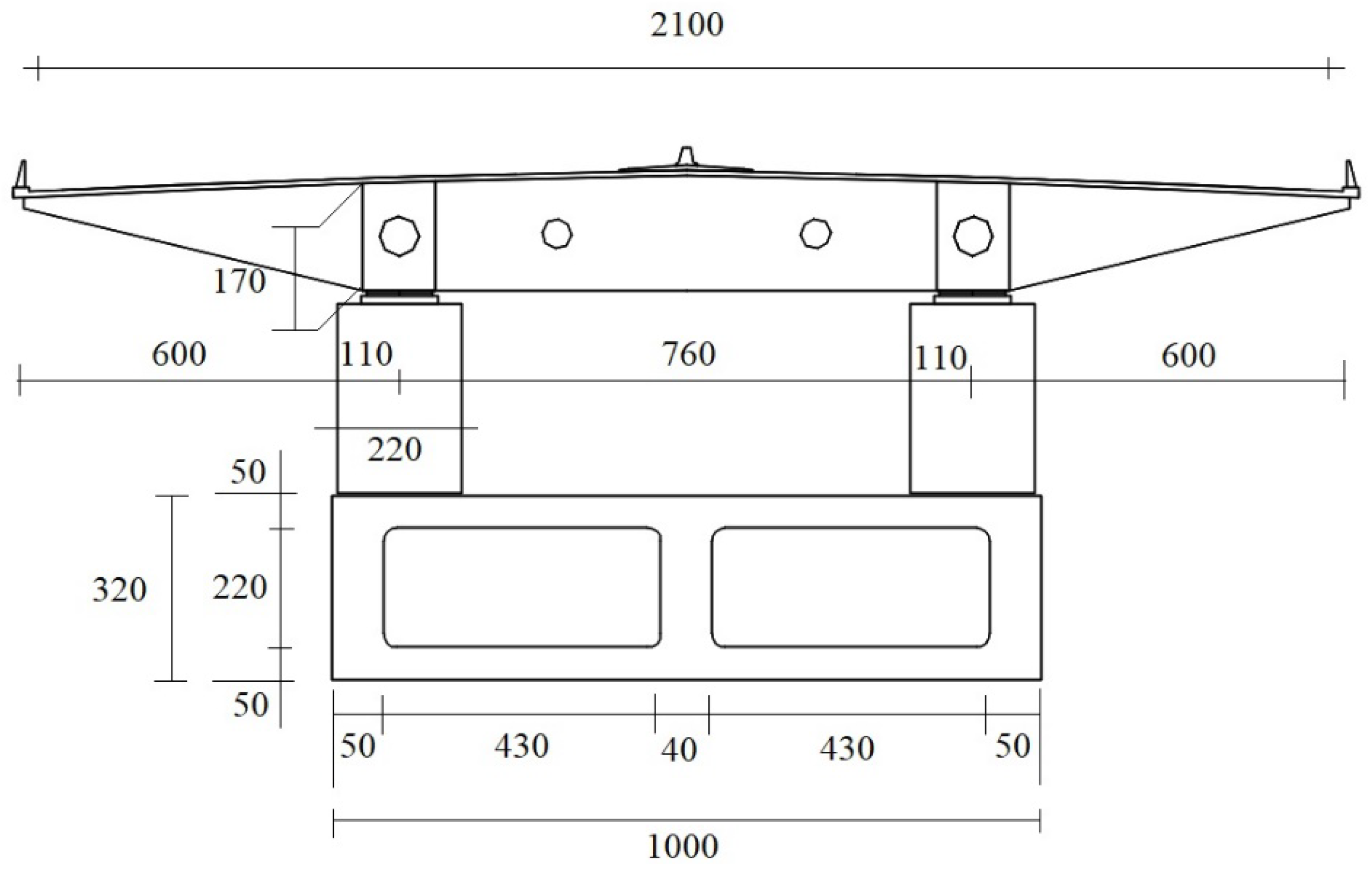
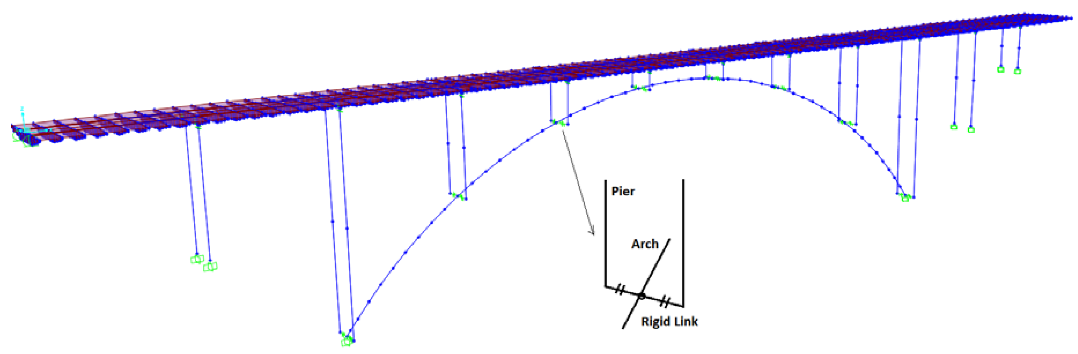
2. Structure of the Representative Bridge Used in the Case Study

An upper-deck RC arch bridge design was designed for the case study analyses (Figure 1). A response spectrum analysis (RSA) was performed when designing the bridge components based on the AASHTO [19] specifications and the Caltrans Seismic Design Criteria [20]. The design spectrum provided in the AASHTO specification for a peak ground motion of 0.35 g, which is representative of a strong earthquake intensity level, and a site class of D was selected.

The reinforced concrete arch of the bridge consists of a double cell-box cross-section with a constant outer dimension (b × h) of 10 m × 3 m (Figure 2). The total length of the bridge was taken to be 400 m, with a reinforced concrete arch length of 212 m and a rise at the crown of 52 m, giving a rise-to-span ratio of 0.25.

A triple-box cross-section was utilized close to the arch abutments in order to enhance the shear and bending stiffness of the bridge structure. Vertical RC diagrams were incorporated inside the RC arch at the point where the columns rest on the arch. Figure 2 shows the transverse section of the model bridge. The composite superstructure, which is 21 m wide and 2.10 m high, consists of a 25 cm reinforced concrete deck-plate supported by two steel box-shaped girders placed 4 m apart. Fixed supports are assumed at the springings of the arch and at the bottom of piers P2, P11 and P13 to represent the foundation over a bedrock site. This is a widely accepted approach used for the majority of arch bridges; the effect of soil-structure interactions are also generally neglected [11,12,13]. The composite deck is supported on longitudinal movable bearings located at the abutments and at the stiff short central piers P5–P8 and P12 (Figure 1). As shown in Figure 2, two types of movable bearing are modeled, namely pinned connections and sliding bearings that support the vertical action only. The bridge deck is highly flexible and may thus experience significant horizontal displacement during a major earthquake event. Any large displacement will result in adverse impacts on all the fixed bearings; hence, viscous dampers of the type developed by Žderić et al. [24] as shown in Figure 3, each with a 2000 KN capacity, are included in the model at both ends of the deck in order to reduce the seismic response of the bridge. These nonlinear Fluid Viscous Dampers (NFVD) were modeled here using the following practical relationship between the internal force acting on the damper, F(N), and the Velocity, V (in m/s) derived experimentally by Seleemah and Constantinou [25]:

$$F=C{V}^{n}sgn(V)$$

(1)

where C (N(sm⁻¹)ⁿ) is the damping constant; velocity exponent, n, defines the type of device and introduces the nonlinearity of viscous damper; and sgn is sign or signum function which is used for defining the sign of a real number. The mechanical characteristics of the damper [24] used in the present study are modeled with n and V values of 0.40 and 0.34 (m·s⁻¹), respectively. Figure 3 shows a fluid viscus damper of the type typically used in bridge abutments.

A total of 13 double columns, shown in cross-section in Figure 4, were defined to support the composite deck. The transverse distance between the columns is 7.60 m, which matches the girder spacing in the superstructure.

European concrete classes [26] C45/55 and C35/45, with strengths in compression of 45 MPa and 35 MPa, respectively, were utilized for the arch and columns. The modulus of elasticity for both concrete materials was 3600 GPA. In this study, only unconfined concrete was used for the bridge components so as to provide conservative design. It should be mentioned that in the investigation by Salonga and Gauvreau [16] the bridge with span length of 400 m was at the second position in their collection of 55 RC arch bridges sorted from largest to smallest span lengths. Therefore, the selected bridges can be considered as a typical long-span RC arch bridge.

3. Modeling the Forces Acting on the Representative Bridge

The three-dimensional analytical model of the reinforced concrete (RC) arch bridge described above was developed using CsiBridge V20 [27] software. Figure 5 shows the resulting three-dimensional finite element model of the bridge. Two-node frame elements, with three translational and three rotational degrees of freedoms (DOF) at each node, were applied to model the RC arch and piers of the bridge.

Based on the bridge geometry discussed in the previous section, the foundations of the piers were assumed to determine the level of base fixity [20]. The height of the piers was defined according to the Caltrans Seismic Design Criteria [18]: separate segments at the top and bottom of each pier with a length D_c.g were used to represent the portion embedded in the superstructure or arch, defined in terms of the difference between the bottom flange and vertical centroid of the cross-section of the superstructure or RC arch (Figure 6), and a rigid offset assigned.

In order to enhance the participation of higher modes, additional nodes were defined at the mid-heights of P2–P3 and P8–P10. The use of effective cross-section properties is a common practice recommended by the Caltrans Seismic Design Criteria [20], anticipating the development of early cracks developing in reinforced concrete piers due to gravity and lateral loads. Therefore, for the seismic analysis of the RC arch bridges the effective inertia of the piers was decreased to 70% of the gross section for the entire length of each element. The torsional moment of inertia for piers was modified according to Equation (2) proposed by the American Concrete Institute’s Building Code Requirements for Structural Concrete (ACI 318-14) [28] to take into account the effect of the reduction in torsional stiffness after cracking:

$$J_{eff}=0.20J_g$$

(2)

where J_eff is the effective torsional stiffness of the piers and J_g is the torsional reduction in the gross cross-section. A modifying factor was also applied to the gross cross-sections of the piers and the arch to allow for the combined effects of flexural and axial load in predicting the shear capacity of ductile members. Equation (3) proposed in Section 3.6 of the Caltrans Seismic Design Criteria [20] was then used to obtain the shear modification factor as follows:

$$A_{v,eff}=0.80A_{v,g}$$

(3)

where A_v,eff is the effective shear area and A_v,g is the shear area of the gross cross-section of the frame elements. The values of A_v,g and J_g were calculated automatically by CsiBridge [27] based on the cross section geometry. In order to develop a realistic model of the superstructure, the deck slab was modeled as four-node shell elements with six degree of freedom at each node, located at the centroid of the deck. Frame elements were applied to model the box-shaped girder located at the centroid of the members [26]. The transverse steel plates were modeled as a shell element supported by stiff U-shaped profiles located along the edges and at specified locations on the plates. The floor-system members were connected using offsets and massless rigid links within the CsiBridge program. The compressive stress-strain relationship developed by Mander et al. [29] was used for the concrete materials. With regard to the bridge loads, the area of the longitudinal reinforcements for the piers and RC arch were taken to be between 3.5% and 4.5% of their gross cross-section areas. The transverse rebars were designed as ϕ 14 mm at 100 mm for the piers and ϕ 18 mm at 100 mm for the RC arch.

4. Case Study of a Representative Bridge

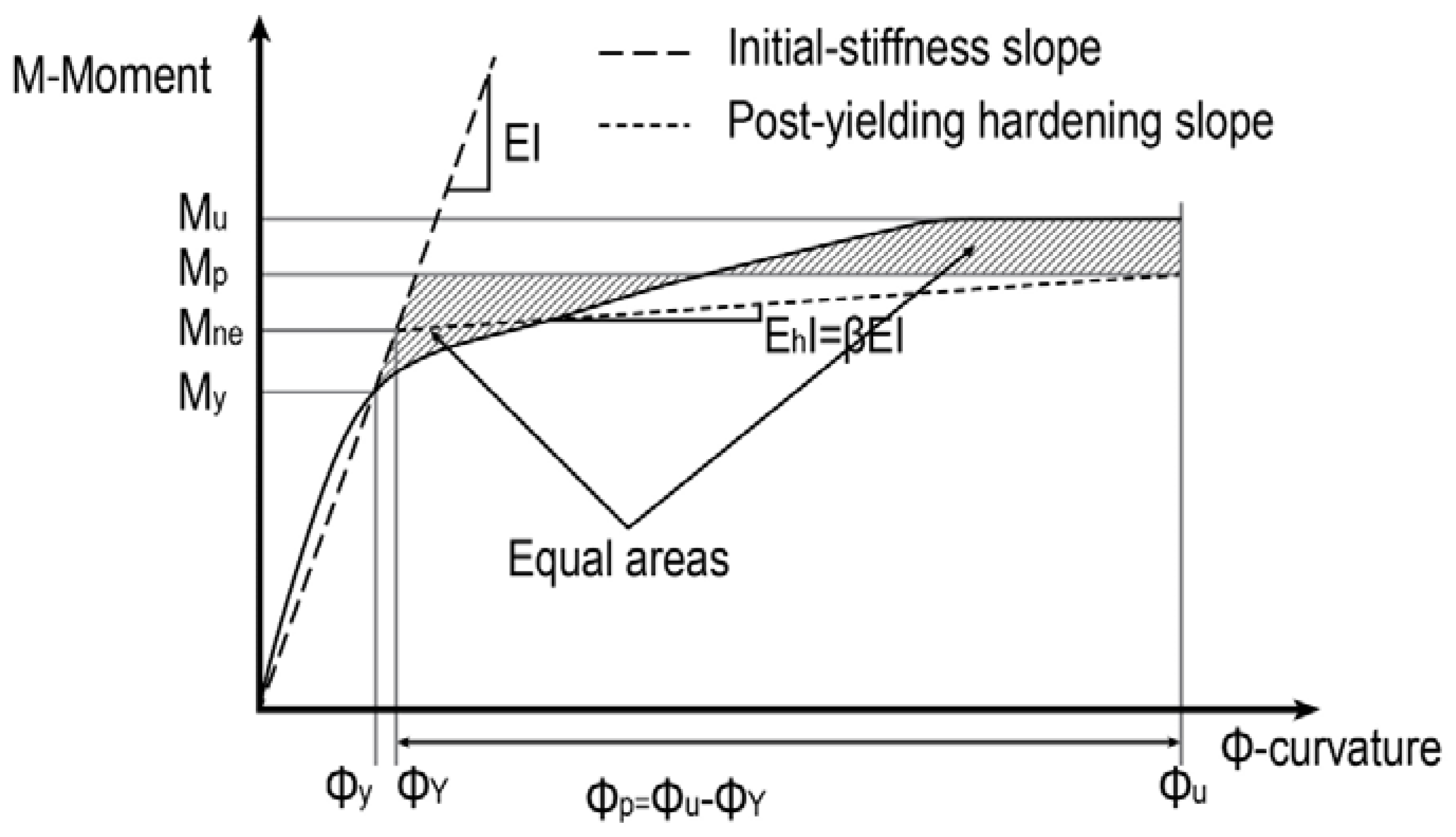
4.1. Moment-Curvature Analysis for Piers

Based on the Caltrans Seismic Design Criteria [20], a moment-curvature (M-φ) analysis was performed for all the ductile concrete members in order to determine the plastic moment capacity of the bridge. A complete moment-curvature analysis also indicates the strength reduction beyond the peak point when the strain-softening characteristics of the concrete are taken into account. The M-φ curve was idealized here using an elasto-perfectly plastic model to determine the plastic flexural capacity of cross section, although a bilinear model capable of accounting for the strain hardening of steel may be preferable in some cases. Figure 7 shows the moment-curvature (M-φ) relationship for a structure. The value of the yield point (φ_y, M_y), the nominal point (φ_Y, M_ne), the ultimate capacity (φ_u, M_u), the plastic capacity (φ_u, M_p) and the curvature ductility (µ_ϕ= φ_u/φ_y) can all be calculated based on a moment-curvature analysis of the bridge’s piers when subjected to a certain level of dead load on the piers and their self-weights.

According to ACI 318-14 [30], the dead load corresponds to a column with a P/P_n ratio between 0.50 and 0.35. Here, P_n is the nominal bearing capacity f’_cA_g, where A_g denotes the cross section of the column and f’_c is the concrete compressive strength. The SD-Section designer program supported by the CsiBridge software was then used to conduct the M-ϕ analysis based on the Caltrans Seismic Design Criteria [20].

4.2. Assigning the Plastic Hinges

The nonlinearity and hysteretic behavior was evaluated by assigning plastic fiber hinges to pre-estimated locations on the piers and RC arch. This fiber hinge option, which automatically adjusts the bending capacity of piers in all directions based on fluctuations in the pier axial loads, is a convenient way to model plastic hinges with sufficient accuracy for our purposes. The M-φ relationship was developed using an assigned fiber hinge that permits all bending directions with various levels of axial force. The SD-designer then calculated the interaction between the axial force and biaxial moment based on the stress-strain relationship assigned to discretized fibers in the member cross-sections. The lengths of the plastic fiber hinges were determined based on Section 7.6.2 of the Caltrans Seismic Design Criteria [18]; these were inserted into the model as individual segments at pre-determined locations. The length of the plastic zone (L_p) was obtained based on AASHTO [19] as follows:

$$L_p=0.08L+0.022f_{ye}{d}_{bl}\ge 0.044f_{ye}{d}_{bl}$$

(4)

where L denotes the length of the pier from the point of maximum moment to the point of moment contraflexure (m), and f_ye and d_bl are the effective yield strength (MPa) and diameter (mm), respectively, of the longitudinal reinforcements. The concrete fibers were placed at the geometric centroids of each of the concrete areas. As more than one longitudinal reinforcement may be lumped at a single location, the fibers were also assumed to be located at the centroid of the bar bundle. The recommendations for pier cross section fiber discretization presented by Berry and Eberhard [31] were used to determine the number of fibers required to represent the cross-section configuration with adequate accuracy.

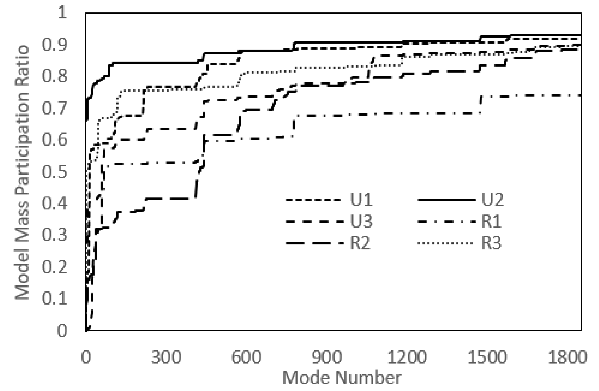
5. Bridge Modal Analysis

Modal analysis is used to determine the undamped free-vibration mode shapes and frequencies of structures. These natural modes provide an excellent insight into structural behavior and can also be used as the basis for response-spectrum analyses (RSA) of bridges.

Table 1. Results of the free-vibration eigenvalue analysis.

(a) Mass Participation Factors
Mode No.	Period (s)	Translational Masses (%)			Rotational Masses (%)
		L	T	V	L	T	V
1	2.34	7.3 × 10−8	6.6 × 10−1	1.0 × 10−7	2.8 × 10−1	6.6 × 10−8	4.4 × 10−4
2	1.66	1.1 × 10−1	2.6 × 10−6	5.6 × 10−6	3.8 × 10−7	8.2 × 10−2	1.8 × 10−7
3	1.20	2.5 × 10−7	2.6 × 10−3	1.6 × 10−9	1.4 × 10−3	2.4 × 10−8	5.0 × 10−1
4	1.08	2.2 × 10−2	3.1 × 10−6	2.1 × 10−2	7.0 × 10−6	1.4 × 10−3	2.1 × 10−6
5	0.80	1.6 × 10−7	1.7 × 10−6	9.4 × 10−5	1.0 × 10−1	1.8 × 10−6	4.9 × 10−5
6	0.71	3.3 × 10−2	5.6 × 10−5	1.9 × 10−3	3.7 × 10−5	3.2 × 10−3	5.7 × 10−6
7	0.64	1.6 × 10−2	1.4 × 10−5	2.6 × 10−3	4.9 × 10−6	4.4 × 10−2	1.7 × 10−6
8	0.63	2.4 × 10−7	6.4 × 10−2	9.6 × 10−7	3.3 × 10−3	4.2 × 10−6	3.5 × 10−4
9	0.59	3.1 × 10−7	1.7 × 10−6	1.0 × 10−8	3.1 × 10−4	1.0 × 10−6	1.0 × 10−3
10	0.55	1.5 × 10−7	6.8 × 10−4	3.4 × 10−5	3.4 × 10−4	6.2 × 10−7	1.5 × 10−2
11	0.52	3.4 × 10−7	1.7 × 10−4	1.2 × 10−5	1.8 × 10−4	6.4 × 10−6	1.1 × 10−3
12	0.52	3.0 × 10−3	3.7 × 10−4	1.9 × 10−4	8.3 × 10−5	3.6 × 10−4	6.1 × 10−3
13	0.51	3.7 × 10−1	1.5 × 10−5	4.7 × 10−3	8.8 × 10−8	2.9 × 10−2	3.0 × 10−5
14	0.50	1.8 × 10−5	1.3 × 10−5	1.9 × 10−4	1.1 × 10−4	6.8 × 10−5	3.0 × 10−4
15	0.48	3.2 × 10−5	1.6 × 10−4	1.6 × 10−3	7.8 × 10−4	6.4 × 10−5	2.6 × 10−5
61	0.31	1.9 × 10−5	4.0 × 10−4	1.8 × 10−1	1.2 × 10−3	7.4 × 10−4	3.1 × 10−7
441	0.13	9.0 × 10−8	7.8 × 10−6	4.1 × 10−6	1.1 × 10−4	8.3 × 10−2	9.2 × 10−9
1850	0.03	2.1 × 10−5	6.7 × 10−8	5.0 × 10−8	2.2 × 10−8	7.6 × 10−5	2.4 × 10−9
(b) Percentage of Modal Mass Participation
Mode No.	Period (s)	Translational Masses (%)			Rotational Masses (%)
		L	T	V	L	T	V
1	2.34	0	0.66	0	0.27	0	0
2	1.66	0.11	0.66	0	0.27	0.08	0
3	1.2	0.11	0.66	0	0.28	0.08	0.5
4	1.08	0.13	0.66	0	0.28	0.09	0.5
5	0.8	0.13	0.66	0	0.38	0.09	0.5
6	0.71	0.17	0.66	0	0.38	0.1	0.5
7	0.64	0.18	0.66	0	0.38	0.14	0.5
8	0.63	0.18	0.73	0	0.39	0.14	0.51
9	0.59	0.18	0.73	0	0.39	0.14	0.51
10	0.55	0.18	0.73	0	0.39	0.14	0.52
11	0.52	0.18	0.73	0	0.39	0.14	0.52
12	0.52	0.18	0.73	0	0.39	0.14	0.53
13	0.51	0.56	0.73	0.01	0.39	0.17	0.53
14	0.5	0.56	0.73	0.01	0.39	0.17	0.53
15	0.48	0.56	0.73	0.01	0.39	0.17	0.53
61	0.31	0.58	0.79	0.32	0.42	0.32	0.66
441	0.13	0.81	0.85	0.67	0.55	0.51	0.76
1850	0.03	0.91	0.93	0.9	0.74	0.88	0.89

L: Longitudinal, T: Transverse, V: Vertical directions.

shows the translational and rotational modes obtained from an eigenvalue analysis of the model RC arch bridge in the current study. The bolded values indicate the dominant modes in each direction. The data in Table 1 confirm that the translational mode in the transverse direction is dominant in the first mode, which is associated with the maximum value of the rotational mode about the longitudinal axis. This means that the first natural (fundamental) mode of the bridge structure is a coupled mode consisting of both a transverse mode and a rotational mode. The rotational mode about the vertical axis is extracted from the third vibrational mode. The dominant mode shape and modal frequencies for all translational and rotational directions are shown in Figure 8.

The number of modes considered in the analysis must be sufficient to achieve at least a 90% mass participation in the longitudinal and torsional directions of the bridge [19,20,21]. A minimum of 1850 modes were therefore considered for the response-spectrum (RSA) and time-history (THA) analyses in this investigation, as shown in Table 1. However, due to space limitations, only the first 15 modes of vibration plus modes 61 and 441, which had the highest mass participation in the vertical translation and transversal rotation, respectively, and the last mode, which satisfied the 90% minimum modal participation, are presented here. To provide a better understanding, the participation of various modes of vibration resulting from an eigenvalue analysis are drawn in terms of their mass fractions in Figure 9.

6. Ground Motion Database

Both record selection and scaling are equally important processes for successful seismic analyses of the structures. Apposite selection of the records considering the hazard conditions for a given site helps to increase accuracy by achieving better estimates of the structural actions. Before scaling ground motions, it is necessary to define the hazard conditions associated with a given site either through deterministic or probabilistic site-specific hazard analysis or alternatively using the seismic hazard maps. The parameters to be considered in identifying the scenario conditions are those that have the most influence on ground motion spectral shape, which includes the magnitude range of anticipated significant event, distance range of the site from the causative fault, site-condition (site-geology generally described by average shear-wave velocity within 30 m), and directivity effect [30]. In this study, the model RC arch bridge was subjected to real world near-field and far-field ground motions extracted from the Pacific Earthquake Engineering Research (PEER) database [31]. Ground motion records from earthquakes in the magnitude (M_w) range of 6.00 to 7.5 within 10 km and 100 km of the causative fault plane were selected as near-field and far-field earthquakes, respectively. Relevant information from the ground motion database, including the station, magnitude, earthquake components, distance from the fault and peak ground acceleration (PGA) is presented in

Table 2. Near field ground motion database.

No.	Year	Earthquake	Mw	Mech a	Station	Dist b	PGA (g)
1	1979	Imperial Valley-06	6.53	SS	EC County Center FF	7.31	0.35
2	1979	Imperial Valley-06	6.53	SS	El Centro Array #7	1.56	0.51
3	1986	N. Palm Springs	6.06	RO	North Palm Springs	4.04	0.84
4	1994	Northridge-01	6.9	REV	Rinaldi Receiving	6.50	0.62
5	1994	Northridge-01	6.69	REV	Sylmar—Converter	5.35	0.52
6	1995	Kobe_Japan	6.90	SS	Takarazuka	1.27	0.71
7	1995	Kobe_Japan	6.90	SS	Takatori	2.47	0.39
8	1992	Erzican_Turkey	6.69	SS	Erzican	4.38	0.57

^a Fault mechanism: REV reverse, SS strike-slip, OB oblique, RO reverse-oblique. ^b Closest distance to fault rupture (km).

and

Table 3. Far field ground motion database.

No.	Year	Earthquake	Mw	Mech a	Station	Dist b	PGA (g)
1	1978	Tabas	7.35	REV	Ferdows	91.40	0.41
2	1952	Kern County	7.36	REV	Taft Lincoln School	38.89	0.44
3	1994	Northridge-01	6.69	REV	La Puente—Rimgrove	56.59	0.32
4	1994	Northridge-01	6.69	REV	Downey—Co Maint	46.74	0.41
5	1999	Kocaeli	7.51	SS	Ambarli	69.62	0.45
6	1987	Whittier Narrows	5.99	RO	Tarzana—Cedar Hill	41.22	0.61
7	1956	El Alamo	6.80	SS	El Centro Array #9	121.3	0.31
8	1994	Northridge-01	6.69	REV	Montebello—Bluff Rd.	45.30	0.39

^a Fault mechanism: REV reverse, SS strike-slip, OB oblique, RO reverse-oblique. ^b Closest distance to fault rupture (km).

.

The ground motion types selected for this study were from site class D of the AASHTO [19] specification, with an average shear wave velocity for the top 30 m of soil, Vs₃₀, in the range of 185 m/s to 365 m/s. The ground motion values were then scaled to have similar recorded amplitudes; hence, the average value of 5% damped response spectra for the suit of records was not less than the design response spectrum of the site for period ranging from 0.2T to 1.5T [32], where T is the period corresponding to the fundamental mode of the bridge. The “matched to response spectrum” option available in the ETABS V16.2.1 [33] software was utilized to scale the recorded ground motion values. Figure 10 shows the 5% damped response spectra for the longitudinal and transverse components of the scaled record; the design spectra recommended by AASHTO [19] and the average response spectrum are also shown for comparison.

As the data presented in Figure 10 show, the scaling culminates in a geometric mean spectrum that closely matches the target spectrum over the significant range of the period for the PEER [32] methodology. The comparison of the AASHTO design spectra and the average longitudinal and transverse responses of the recorded ground motion thus provide a better understanding of the relationship between spectral amplitudes and structural period.

7. Dynamic Analysis

According to AASHTO [19], historical analyses of the nonlinear response should generally be applied for critical/essential structures such as RC arch bridges. Here, the dynamic analysis was performed in two steps. In the first step, a nonlinear static analysis was carried out by applying the gravity loads progressively, using time increments of 0.1 s. The second step consisted of performing a nonlinear Time-History Analysis (THA) of the bridge when subjected to all scaled ground motion records. Here, all 1850 modes needed to capture 90% of the mass participation in both the longitudinal and transverse directions [19] were taken into account. For the nonlinear direct-integration time history analysis, both material and geometric (large displacement effects) nonlinearities were considered. Although a variety of common methods are provided in the CsiBridge software for conducting direct-integration time history analysis, the Hibler-Hughes-Tylor alpha (HHT) technique [34] was used in this study. In order to enhance the accuracy, the smallest possible time-steps and alpha values close to zero were applied along with Rayleigh damping, a function of the mass and stiffness of the structure. Based on the natural period of the bridge extracted from the eigenvalue analysis and imposing a 5% modal damping ratio, the mass and stiffness proportion coefficients were determined to be 0.151 and 0.0155, respectively.

8. Seismic Performance Evaluation

From an earthquake-engineering viewpoint, determining the critical section of structure and predicting the location of maximum displacement or stress are the most significant issues.

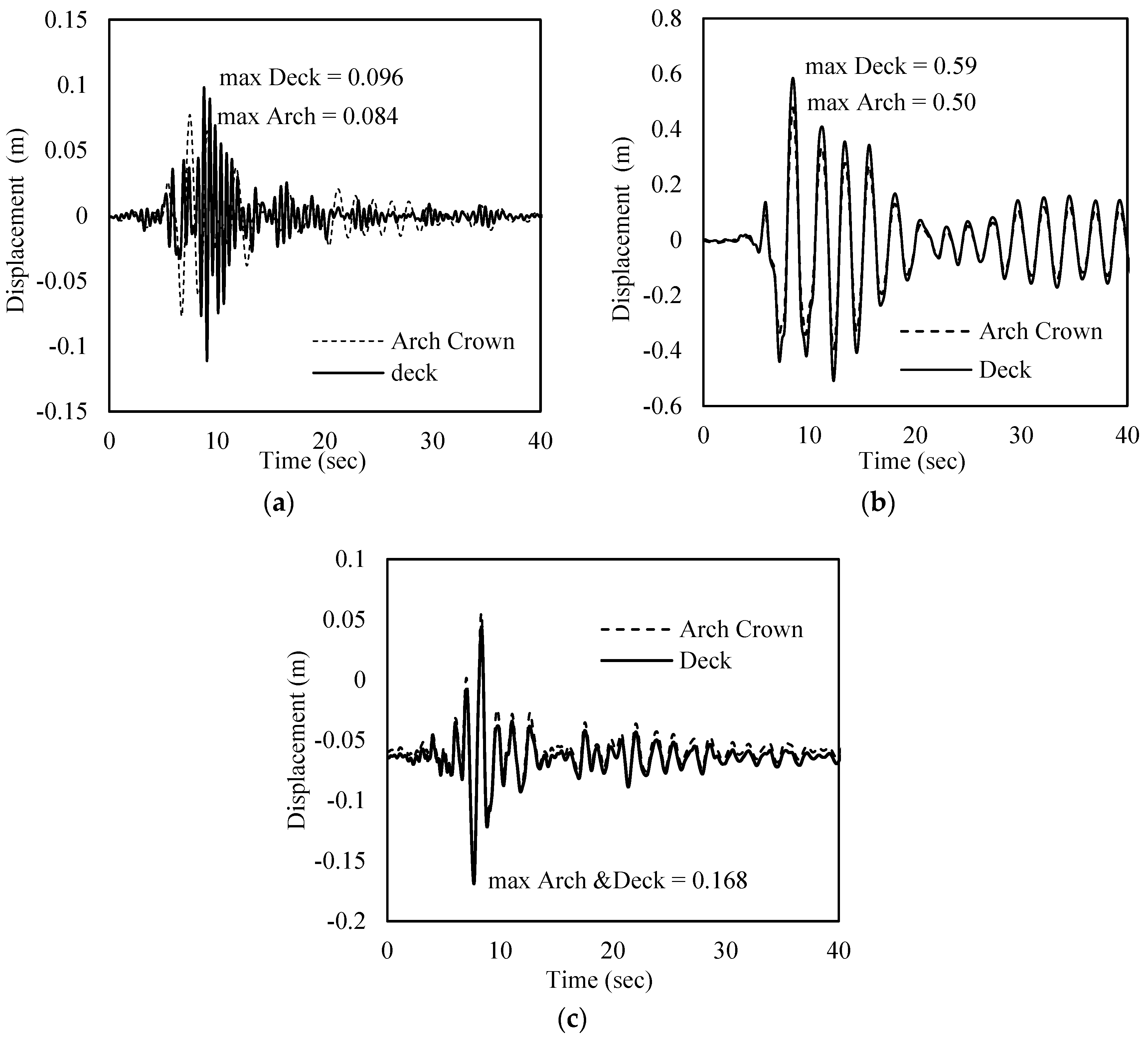
8.1. Seismic Displacement Demand Estimation

The estimated maximum seismic displacement demand at the deck and arch crown of a model bridge subjected to the scaled ground motions listed in Table 2 and Table 3 are presented in

Table 4. Maximum displacement values at deck and arch crown for near-field earthquakes.

No.	Station	Deck (m)			Arch Crown (m)
		L	T	V	L	T	V
1	EC County	0.080	0.480	0.164	1.110	0.509	0.170
2	El Centro #7	0.096	0.592	0.168	0.084	0.503	0.168
3	North Palm	0.111	0.678	0.247	0.108	0.562	0.192
4	Rinaldi	0.120	0.765	0.180	0.103	0.615	0.174
5	Sylmar	0.123	0.406	0.155	0.077	0.317	0.154
6	Takarazuka	0.103	0.483	0.165	0.105	0.596	0.165
7	Takatori	0.131	0.728	0.158	0.098	0.581	0.163
8	Erzican	0.103	0.732	0.156	0.091	0.590	0.158
9	Average	0.112	0.627	0.177	0.224	0.545	0.165

L: Longitudinal, T: Transverse, V: Vertical directions.

and

Table 5. Maximum displacement values at deck and arch crown for far-field earthquakes.

No.	Station	Deck (m)			Arch Crown (m)
		L	T	V	L	T	V
1	Ferdows	0.127	0.451	0.150	0.077	0.353	0.148
2	Taft Lincoln	0.087	0.593	0.168	0.098	0.470	0.171
3	La Puente	0.093	0.316	0.122	0.067	0.240	0.125
4	Downey-Maint	0.087	0.670	0.167	0.092	0.527	0.171
5	Ambarli	0.118	0.470	0.152	0.103	0.373	0.152
6	Tarzana	0.109	0.335	0.122	0.055	0.280	0.112
7	El Centro #9	0.101	0.540	0.162	0.091	0.433	0.162
8	Montebello	0.090	0.542	0.170	0.091	0.423	0.174
9	Average	0.101	0.490	0.151	0.084	0.388	0.151

L: Longitudinal, T: Transverse, V: Vertical directions.

, respectively. For near-field ground motion (Table 4), the maximum vertical and transverse displacements for the deck and arch crown were from Earthquakes 3 and 4, respectively, while the largest displacements in the longitudinal direction were obtained under Earthquakes 7 and 1. For far-field earthquakes (Table 5), the dynamic analysis revealed that bridges subjected to ground motion from Earthquake 2 exhibited the greatest displacement in the vertical and transverse directions of the bridge superstructure, while the largest displacement values were obtained in Earthquakes 5, 4 and 8 for the longitudinal, transverse and vertical directions, respectively.

The average values of the maximum displacement are also shown in Table 4 and Table 5. Interestingly, the listed values for the maximum displacement of the deck do not occur at the same locations. Figure 11 indicates the maximum displacement for the deck and arch crown histories of a bridge subjected to Imperial Valley-06 ground motion recorded at the Array #7 station. A significant relative difference between the deck and arch displacement can be observed in longitudinal direction, while the deck and arch displacement in the other directions show almost identical results for the time history analysis. This indicates that no significant residual deck displacement remains at the end of the analysis; hence, no damage has occurred in either the piers or the arch, which play the greatest role in supporting the internal forces of the deck. Although the maximum vertical displacement of the deck and arch is 0.178 m, by the end of the time-history analysis only a residual displacement of 0.061 remains, which is effectively negligible.

8.2. Distribution of Internal Forces and Bending Moments

Figure 12 indicates the distribution of the mean internal forces in the arch of a bridge subjected to a near-field earthquake. The shear forces and bending moments for different directions in the RC arch are identified by RF_i and RM_i, respectively. The in-plane shear force and bending moment in the normal direction to the axis of the arch are denoted by RF₂ and RM₃, respectively, while RF₃ and RM₂ are, respectively, the out-of-plane shear force and bending moment in the transverse direction of the arch. Figure 12 shows that the maximum axial forces are obtained at the arch’s springings (arch abutments). The axial forces at the arch crown can be up to 35% lower than those at the springings. The shear forces in both directions (in-plane and out-of-plane) are distributed approximately uniformly along the RC arch. Figure 12b shows that the variation in the out-of-plane bending moment, RM₂, is accompanied by a steep gradient near the arch’s springings and a local maximum at the arch crown of the bridge; the in-plane bending moment, RM₃, is distributed along the arch and follows the same trend, albeit with lower values. The same variation in the patterns exhibited by the shear force and bending moment distributions are produced in bridges subjected to far-field earthquake, but due to space limitation these are not presented here.

8.3. Demand/Capacity Evaluation

The Demand/Capacity Ratios (DCR) from the response spectrum (RSA), equivalent static method (ESA) and nonlinear time history (NTHA) analyses of the model bridge subjected to near- and far-field ground motions are presented in

Table 6. Demand/Capacity Ratios for bridges under near-field earthquakes, Equivalent Static (ESA) and Response spectrum (RSA) analyses.

No.	P1		P2		P3		P4		P5		P6		P7		P8		P9		P10		P11
	L	R	L	R	L	R	L	R	L	R	L	R	L	R	L	R	L	R	L	R	L	R
1	0.77	0.85	0.63	0.69	0.92	0.95	0.70	0.31	0.46	0.18	0.48	0.18	0.81	0.41	0.65	0.70	0.52	0.53	0.61	0.61	0.54	0.57
2	0.79	0.91	0.66	0.68	0.95	0.95	0.73	0.32	0.48	0.17	0.47	0.18	0.83	0.44	0.66	0.73	0.56	0.59	0.72	0.72	0.63	0.64
3	0.85	0.95	0.71	0.71	0.94	0.96	0.79	0.36	0.63	0.18	0.60	0.19	0.85	0.48	0.74	0.80	0.58	0.60	0.73	0.75	0.65	0.68
4	0.94	0.92	0.77	0.80	0.93	0.95	0.78	0.46	0.65	0.24	0.68	0.20	0.80	0.58	0.85	0.83	0.62	0.59	0.80	0.82	0.66	0.62
5	0.70	0.62	0.54	0.48	0.71	0.72	0.59	0.32	0.44	0.17	0.43	0.16	0.66	0.41	0.62	0.58	0.48	0.41	0.48	0.46	0.47	0.42
6	0.88	0.78	0.69	0.71	0.92	0.94	0.89	0.44	0.96	0.22	0.90	0.22	0.99	0.61	0.76	0.71	0.54	0.52	0.64	0.67	0.56	0.56
6 *	0.87	0.76	0.64	0.63	0.85	0.86	0.83	0.38	0.85	0.16	0.75	0.17	0.90	0.51	0.69	0.63	0.52	0.50	0.56	0.57	0.59	0.55
7	0.88	0.89	0.72	0.70	0.95	0.96	0.87	0.36	0.74	0.17	0.75	0.17	0.95	0.45	0.74	0.70	0.60	0.61	0.73	0.71	0.64	0.63
8	0.81	0.91	0.71	0.71	0.93	0.91	0.76	0.35	0.56	0.17	0.51	0.18	0.82	0.53	0.76	0.79	0.59	0.65	0.78	0.76	0.67	0.66
Avg.	0.83	0.85	0.68	0.68	0.90	0.91	0.76	0.36	0.61	0.19	0.60	0.18	0.84	0.49	0.72	0.73	0.56	0.56	0.69	0.69	0.60	0.60
ESA	0.71	0.74	0.56	0.57	0.72	0.65	0.59	0.14	0.58	0.09	0.53	0.46	0.57	0.21	0.61	0.60	0.51	0.52	0.74	0.73	0.72	0.71
RSA	0.64	0.64	0.51	0.51	0.77	0.76	0.70	0.47	0.80	0.12	0.78	0.13	0.78	0.63	0.51	0.52	0.44	0.44	0.53	0.53	0.52	0.52

* Demand/Capacity ratio under horizontal and transverse components.

and

Table 7. Demand/Capacity Ratios for bridges under far-field earthquakes, Equivalent Static (ESA) and Response spectrum (RSA) analyses.

No.	P1		P2		P3		P4		P5		P6		P7		P8		P9		P10		P11
	L	R	L	R	L	R	L	R	L	R	L	L	R	L	R	L	R	L	R	L	R	L
1	0.72	0.79	0.62	0.64	0.78	0.81	0.62	0.32	0.46	0.19	0.49	0.18	0.73	0.43	0.60	0.63	0.45	0.46	0.50	0.51	0.50	0.50
1 *	0.70	0.76	0.58	0.58	0.79	0.76	0.57	0.31	0.40	0.17	0.43	0.16	0.67	0.40	0.55	0.56	0.42	0.44	0.48	0.49	0.48	0.49
2	0.76	0.79	0.64	0.61	0.93	0.91	0.72	0.33	0.49	0.18	0.52	0.19	0.83	0.44	0.71	0.71	0.56	0.53	0.62	0.61	0.55	0.56
3	0.64	0.58	0.56	0.46	0.59	0.55	0.48	0.30	0.38	0.16	0.37	0.15	0.59	0.40	0.51	0.48	0.40	0.38	0.47	0.42	0.47	0.40
4	0.78	0.78	0.66	0.65	0.91	0.90	0.74	0.32	0.56	0.18	0.50	0.17	0.74	0.43	0.75	0.71	0.55	0.57	0.64	0.63	0.57	0.58
5	0.75	0.72	0.65	0.58	0.76	0.82	0.58	0.31	0.42	0.17	0.42	0.16	0.70	0.41	0.59	0.61	0.49	0.45	0.57	0.50	0.50	0.48
6	0.62	0.65	0.51	0.50	0.58	0.55	0.59	0.38	0.66	0.19	0.66	0.18	0.67	0.45	0.51	0.49	0.42	0.40	0.45	0.43	0.45	0.42
7	0.72	0.75	0.58	0.62	0.81	0.84	0.66	0.32	0.45	0.19	0.51	0.18	0.76	0.45	0.60	0.60	0.51	0.49	0.55	0.54	0.53	0.51
8	0.73	0.80	0.61	0.61	0.84	0.86	0.66	0.35	0.49	0.18	0.52	0.18	0.81	0.46	0.63	0.67	0.53	0.51	0.58	0.59	0.58	0.58
Avg.	0.71	0.73	0.60	0.59	0.80	0.80	0.63	0.33	0.49	0.18	0.50	0.18	0.73	0.43	0.61	0.61	0.49	0.47	0.55	0.53	0.52	0.50
ESA	0.71	0.74	0.56	0.57	0.72	0.65	0.59	0.14	0.58	0.09	0.53	0.46	0.57	0.21	0.61	0.60	0.51	0.52	0.74	0.73	0.72	0.71
RSA	0.64	0.64	0.51	0.51	0.77	0.76	0.70	0.47	0.80	0.12	0.78	0.13	0.78	0.63	0.51	0.52	0.44	0.44	0.53	0.53	0.52	0.52

* Demand/Capacity ratio under horizontal and transverse components.

. The results show that the longer piers tend to be more vulnerable to nonlinear interactions between the axial forces and the biaxial bending moment. Maximum axial-bending DCR values of up to 0.92 and 0.96 were found for pier P3 when the bridge was subjected to the Kobe-Takatori and Northbridge-Downey ground motions, respectively, thus representing both near-field and far-field earthquakes. In addition, the DCR values of less than one and the minor differences between the DCR values of the piers obtained from various analyses (ESA, RSA and NTHA) confirm that sufficient ductility, strength, geometries and reinforcement have been provided in the structure designed for this study. It is also possible to conclude that near-field ground motion tends to result in higher DCR values than far-field earthquakes, with the difference between the two being as much as 10%. There is a direct relationship between the PGA and DCR of a bridge under near-field ground motion; consequently, in most cases an earthquake with a higher PGA also is likely to result in larger DCR values. The same relationship does not appear to hold for far-field motions, however. To better understand the DCR distribution for RC arch bridges, Figure 13 presents the DCR for pier and arch ribs of a bridge subjected to the Erzican earthquake. This suggests that nonlinear interactions between axial forces, in-plane and out-of-plane bending for longer piers are more critical. Here, the maximum DCR values obtained for arch ribs were around 0.350, but these are not shown due to space limitations.

The fraction of the input energy dissipated by mechanisms such as modal damping and hysteretic dissipation is considered a useful indicator of the damage level of a structure [35]. The percentage of the input energy lost to modal damping and hysteretic energy dissipated is shown in Figure 13. Here, approximately 53% and 57% of the input energy have been dissipated through modal damping when the bridge is subjected to near-field and far-field earthquakes, respectively, associated with the Imperial Valley at EC Country Center and Northbridge at La Puente station.

8.4. Effect of Vertical Acceleration

Significant damage to structures due to vertical excitation has been reported in previous earthquakes such as Northbridge [36]. However, many of the building failures were attributed to brittle failure in the reinforced concrete due to direct compressive failure resulting from the large vertical actions experienced, which is widely disregarded in the seismic design of bridges (Kim et al., [37]). The effect of the vertical acceleration on the dynamic responses of a bridge subjected to the Kobe ground motion at Takarazuka station (PGA = 0.71) and Tabas motion at Ferdows station (PGA = 0.42), representing near and far-field earthquakes, respectively, was therefore investigated in this study. For better understanding, the time-history analysis was performed both with and without taking into account the vertical component of the ground motion. The maximum displacement of the deck and arch crown are presented in

Table 8. Effect of vertical component displacement of the deck and arch crown (DCR).

Earthquake Name			Three Orthogonal Accelerations	Two Horizontal Accelerations	Difference (%)
Kobe (Takarazuka)	Arch	L	0.105	0.098	6.70
		T	0.596	0.535	10.2
		V	0.165	0.041	75.2
	Deck	L	0.103	0.095	7.76
		T	0.483	0.442	8.50
		V	0.165	0.045	72.7
Tabas (Ferdows)	Arch	L	0.077	0.070	9.10
		T	0.353	0.322	8.78
		V	0.148	0.038	74.3
	Deck	L	0.127	0.116	8.66
		T	0.451	0.418	7.31
		V	0.150	0.039	74.00

L: Longitudinal, T: Transverse, V: Vertical directions.

.

The DCR values for a bridge subjected to the Kobe earthquake without taking into account the vertical component is also indicated in Table 8. In this case, the highest discrepancies of about 8%, 10.2% and 72.2% were obtained for displacements in the longitudinal, transverse and vertical direction. When the vertical component of ground motion was taken into account there was a significant impact on the DCR values of the bridge, with a maximum discrepancy of 17% being reached in pier P6, and the same pattern was shown in the results for far-field earthquake ground motion (Table 6 and Table 7). This indicates that the vertical acceleration plays an important role in the seismic behavior of a bridge and hence it is strongly recommended that all three orthogonal components of ground motion should be included in seismic analyses and design of RC arch bridges.

9. Conclusions

The structural performance of a reinforced concrete arch bridge subjected to the action of earthquake ground motion was investigated in this study. The finite element model used here was developed based on the design criteria in the AASHTO [19] specifications. An eigenvalue analysis, together with a series of dynamic time history analyses, was performed to clarify the details of the seismic behavior of this type of bridge. The concept of Demand to Capacity Ratios (DCR) was also evaluated in order to provide an initial estimate of the seismic performance of RC arch bridges and the effect of the vertical component of ground motion on the dynamic characteristics of such bridges was considered. Based on the results obtained, the following conclusions can be drawn:

• The eigenvalue analysis demonstrated that an unexpectedly high number of modes of vibration contributed to the seismic behavior of the model RC arch bridge. In order to achieve the 90% modal contribution recommended by the AASHTO [19] specifications, it was necessary to include 1850 modes of vibration.
• The DCR less than unity indicated that the arch bridge modeled in this study showed no sign of gross damage under either near- or far-field ground motion, although insignificant hazard levels for the DCR were reported for two piers. This is likely due to installing fixed bearings at both ends of the model bridge.
• A significant relative difference between the deck and arch displacement can be observed in longitudinal direction, while the deck and arch displacement in the other directions show almost identical results for the time history analysis. This indicates that no significant residual deck displacement remains at the end of the analysis; hence, no damage has occurred in either the piers or the arch, which play the greatest role in supporting the internal forces of the deck.
• The diagram representing the distribution of axial forces and out-of-plane bending moments along the main arch shows that for both near- and far-field ground motions, the average of maximum values calculated from the time history analyses has increased with a rather steep gradient near the abutment of the RC arch. The distribution of the in-plane shear force is almost uniform along the RC arch.
• The average discrepancies, 53%, for displacement in vertical direction and up to 16% in DCR were observed when considering the vertical component of earthquake in dynamic analysis. It was concluded that ignoring the effect of the vertical component of ground motion highlighted the importance of including this effect when modeling the dynamic responses of long-span arch bridges. Hence, it is strongly recommended that this be taken into account when designing RC arch bridges.

References

1. Chen, B.; Ye, L. An overview of long span concrete arch bridges in China. In Proceedings of the Chinese-Croatian Joint Colloquium, Long Arch Bridges, Brijuni Islands, Croatia, 10–14 July 2008; Fuzhou University: Fuzhou, China, 2008. [Google Scholar]
2. Radic, J.; Kindij, A.; Ivankovic, A.M. History of concrete application in development of concrete and hybrid arch bridges. In Proceedings of the Chinese-Croatian Joint Colloquium, Long Arch Bridges, Brijuni Islands, Croatia, 10–14 July 2008; Fuzhou University: Fuzhou, China, 2008. [Google Scholar]
3. Mantzaris, G.; Pnevmatikos, N.; Tsiboukaki, G.; Mantzaris, A. Standardization of bridge structures for spans up to 100 m. Concr. Plant Int. J. 2010, 3, 164–172. [Google Scholar]
4. Pnevmatikos, N.; Sentzas, V. Preliminary estimation of response of curved bridges subjected to earthquake loading. J. Civ. Eng. Archit. 2010, 6, 1530–1535. [Google Scholar]
5. Chen, B. Long span arch bridges in China. In Proceedings of the Chinese-Croatian Joint Colloquium, Long Arch Bridges, Brijuni Islands, Croatia, 10–14 July 2008; Fuzhou University: Fuzhou, China, 2008. [Google Scholar]
6. Kawashima, K.; Mizoguti, A. Seismic response of a reinforced concrete arch bridge. In Proceedings of the 12th World Conference on Earthquake Engineering, Auckland, New Zealand, 30 January–4 February 2000; New Zealand Society for Earthquake Engineering: Upper Hutt, New Zealand, 2000. [Google Scholar]
7. McCallen, D.; Noble, C.; Hoehler, M. The Seismic Response of Concrete Arch Bridges: With Focus on the Bixby Creek Bridge; Report No.: UCRL-ID-134419; Lawrence Livermore National Laboratory: Springfield, VA, USA, 1999. Available online: https://e-reports-ext.llnl.gov/pdf/236014.pdf (accessed on 15 March 2018).
8. Cetinkaya, O.T.; Nakamura, S.; Takahashi, K. Expansion of a static analysis-based out-of-plane maximum inelastic seismic response estimation method for steel arch bridges to in-plane response estimation. Eng. Struct. 2009, 31, 2209–2212. [Google Scholar] [CrossRef] [Green Version]
9. Torkamani, M.; Lee, H.K. Dynamic behavior of steel deck tension-tied arch bridges to seismic excitation. J. Bridge Eng. 2002, 7, 57–67. [Google Scholar] [CrossRef]
10. Nazmy, A.S. Seismic response analysis of long-span steel arch bridges. Proc. Inst. Civ. Eng. 2003, 156, 91–97. [Google Scholar] [CrossRef]
11. Lu, Z.; Usami, T.; Ge, H. Seismic performance evaluation of steel arch bridges against major earthquakes. Part 2: Simplified verification procedure. Earthq. Eng. Struct. Dyn. 2004, 33, 1355–1372. [Google Scholar] [CrossRef]
12. Usami, T.; Lu, Z.; Ge, H.; Kono, T. Seismic performance evaluation of steel arch bridges against major earthquakes. Part 1: Dynamic analysis approach. Earthq. Eng. Struct. Dyn. 2004, 33, 1337–1354. [Google Scholar] [CrossRef]
13. Kandemir, E.C.; Mazda, T.; Nurui, H.; Miyamoto, H. Seismic retrofit of an existing steel arch bridge using viscous damper. In Proceedings of the Twelfth East Asia-Pacific Conference on Structural Engineering and Construction, Hong Kong, China, 26–28 January 2011; Elsevier: New York, NY, USA, 2011. [Google Scholar]
14. Khan, E.; Sullivan, J.T.; Kowalsky, M. Direct displacement–based seismic design of reinforced concrete arch bridges. J. Bridge Eng. 2014, 19, 44–58. [Google Scholar] [CrossRef]
15. Franetovic, M.; Ivankovic, A.M.; Radic, J. Seismic assessment of existing reinforced-concrete arch bridges. Građevinar 2014, 8, 691–703. [Google Scholar] [CrossRef]
16. Chen, K.; Song, J.Y. Survey and analysis of exiting reinforced concrete ribbed arch bridges. Adv. Mater. Res. 2011, 255–260, 1187–1191. [Google Scholar] [CrossRef]
17. Priestley, M.J.N.; Calvi, G.M.; Kowalsky, M.J. Direct Displacement Based Design of Structures, 2nd ed.; EUcentre Foundation, Istituto Universitario di Studi Superiori di Pavia (IUSS) Press: Pavia, Italy, 2018; ISBN 978-8861980006. [Google Scholar]
18. Salonga, J.; Gauvreau, P. Comparative study of the proportions, form, and efficiency of concrete arch bridges. J. Bridge Eng. 2014, 19. [Google Scholar] [CrossRef]
19. American Association of State Highway and Transportation Officials (AASHTO). Guide Specifications for LRFD Seismic Bridge Design, 2nd ed.; AASHTO: Washington, DC, USA, 2011. [Google Scholar]
20. California Department of Transportation. Caltrans Seismic Design Criteria (SDC), V1.7; California Department of Transportation: Sacramento, CA, USA, 2016.
21. Hatzigeorgiou, G. Ductility demand spectra for multiple near- and far-fault earthquakes. Soil Dyn. Earthq. Eng. 2010, 30, 170–183. [Google Scholar] [CrossRef]
22. Alavi, B.; Krawinkler, H. Behavior of moment-resisting frame structures subjected to near-fault ground motions. Earthq. Eng. Struct. Dyn. 2004, 33, 687–706. [Google Scholar] [CrossRef]
23. Baker, J. Efficient analytical fragility function fitting using dynamic structural analysis. Earthq. Spectra 2015, 31, 579–599. [Google Scholar] [CrossRef]
24. Žderić, Z.; Runjić, A.; Hrelja, G. Design and construction of Cetina arch bridge. In Proceedings of the Chinese-Croatia Joint Colloquium on Long Arch Bridges, Brijuni Islands, Croatia, 10–14 July 2008; Fuzhou University: Fuzhou, China, 2008; pp. 285–292. [Google Scholar]
25. Seleemah, A.A.; Constantinou, M.C. Investigation of Seismic Response of Buildings with Linear and Nonlinear Fluid Viscous Dampers; Technical Report NCEER-97-0004; State University of New York at Buffalo: Buffalo, NY, USA, 1997. [Google Scholar]
26. European Committee for Standardization. Eurocode 2: Design of Concrete Structures Part 1: General Rules and Rules for Buildings; EN1992-1; European Committee for Standardization: Brussels, Belgium, 2004. [Google Scholar]
27. Computer & Structures Inc. (CSI). Integrated 3D Bridge Design Software, v20; CSiBridge Advanced; CSI: Berkeley, CA, USA, 2017. [Google Scholar]
28. Finke, J.E. Static and Dynamic Characterization of Tied Arch Bridges. Ph.D. Thesis, Missouri University of Science and Technology, Rolla, MO, USA, 2016. [Google Scholar]
29. Mander, J.B.; Priestley, J.N.; Park, R. Theoretical stress-strain model for confined concrete. J. Struct. Eng. 1988, 114, 1804–1826. [Google Scholar] [CrossRef]
30. American Concrete Institute. Building Code Requirements for Structural Concrete; Commentary on Building Code Requirements for Structural Concrete (ACI 318R-14); Reported by ACI Committee 318; American Concrete Institute: Farmington Hills, MI, USA, 2005. [Google Scholar]
31. Berry, M.; Eberhard, M.O. Performance Modeling Strategies for Modern Reinforced Concrete Bridge Columns; PEER Report 2007/07; Pacific Earthquake Engineering Research Center, University of California: Berkeley, CA, USA, 2008. [Google Scholar]
32. American Society of Civil Engineers. Minimum Design Loads for Buildings and Other Structures; ASCE Standard ASCE/SEI 7-10; American Society of Civil Engineers: Reston, VA, USA, 2010; ISBN 978-0-7844-1085-1. [Google Scholar]
33. Computer & Structures Inc. (CSI). Integrated Analysis, Design and Drafting of Building Systems; ETABS, v16.2.1; CSI: Berkeley, CA, USA, 2016. [Google Scholar]
34. Hilber, H.M.; Hughes, T.J.; Taylor, R.L. Improved numerical dissipation for time integration algorithms in structural dynamics. Earthq. Eng. Struct. Dyn. 1977, 5, 283–292. [Google Scholar] [CrossRef]
35. Soong, T.T.; Spencer, J. Supplemental energy dissipation: State-of-the-art and state-of-the-practice. Eng. Struct. 2002, 24, 243–259. [Google Scholar] [CrossRef]
36. Papazoglou, A.; Elnashai, A. Analytical and field evidence of the damaging effect of vertical earthquake ground motion. Earthq. Eng. Struct. Dyn. 1996, 25, 1109–1138. [Google Scholar] [CrossRef]
37. Kim, S.J.; Curtis, J.H.; Elnashai, A. Analytical assessment of the effect of vertical earthquake motion on RC bridge piers. J. Struct. Eng. 2011, 137, 252–260. [Google Scholar] [CrossRef]
Figure 1. Longitudinal view of the model RC arch bridge designed for this study. All measurements are in m.
Applsci 08 01243 g001
Figure 2. Cross section of the composite deck and RC arch at the P6 position. All measurements are in cm.
Applsci 08 01243 g002
Figure 3. Typical nonlinear fluid viscous damper [24].
Applsci 08 01243 g003
Figure 4. Cross section of the double piers in the model RC arch bridge. All measurements are in cm.
Applsci 08 01243 g004
Figure 5. Three-dimensional FEA model of the bridge constructed using CsiBridge.
Applsci 08 01243 g005
Figure 6. Pier end locations relative to the top and bottom joints [18].
Applsci 08 01243 g006
Figure 7. Moment-curvature relation.
Applsci 08 01243 g007
Figure 8. CsiBridge output for the first three modes of vibration for the model RC arch bridge. (a) 1st mode (Transverse & symmetric torsion); (b) 2nd mode (Longitudinal); (c) 3rd mode (Transverse & anti-symmetric vertical torsion).
Applsci 08 01243 g008
Figure 9. Mass participation vs. mode number.
Applsci 08 01243 g009
Figure 10. Response spectra of the scaled ground motion records. (a) Near-field ground motion; (b) Far-field ground motion.
Applsci 08 01243 g010
Figure 11. Deck and arch crown displacement histories for Imperial Valley-06 earthquake. (a) Longitudinal direction; (b) Transverse direction; (c) Vertical direction.
Applsci 08 01243 g011
Figure 12. Distribution of the average internal forces in the RC arch due to near-field earthquakes. (a) Axial and shear forces; (b) Bending moments.
Applsci 08 01243 g012
Figure 13. Percentage of input energy dissipated by modal damping and hysteretic dissipation. (a) Near-field earthquakes; (b) Far-field earthquakes.
Applsci 08 01243 g013