Comparative Study of Dynamic Stall under Pitch Oscillation and Oscillating Freestream on Wind Turbine Airfoil and Blade

Abstract

This study aims to assess the dynamic stall of the wind turbine blade undergoing pitch oscillation (PO) and oscillating freestream (OF), respectively. Firstly, a thin-airfoil theoretical analysis was performed to differentiate between these two dynamic effects. During upstroke, PO results in a positive effective airfoil camber, while OF has an additional negative effective airfoil camber, and yet in contrast during downstroke, PO decreases the effective camber, while OF increases the effective camber. Secondly, the equivalence relation between PO and OF is investigated by numerically solving the unsteady Reynolds-averaged Navier-Stokes equations. The difference between PO and OF mainly exists in the linear part of the aerodynamic loads. Because the difference is great at high reduced frequencies or angle of attack (AOA) amplitudes, PO and OF should be treated separately for dynamic stall from different aerodynamic sources. Thirdly, the Beddoes-Leishman dynamic model coupled with Bak’s rotational stall delay model was used to predict the yawed responses of the blade section. The obtained results show different aerodynamic responses between PO and OF, although consideration of rotational augmentation can greatly improve the accuracy of the lift and drag coefficients. To improve the understanding and coupling modeling of rotational augmentation and dynamic stall, an extended analysis of the coupled effect was performed as well.

1. Introductions

Horizontal axis wind turbines (HAWTs) often experience unsteady air loads, to which wind turbine failures, reduced machine life, and increased operating maintenance are all directly linked. However, deep understanding and accurate prediction of the unsteady blade air loads and rotor performance face many challenges [1], among which ‘dynamic stall’ is of particular significance. Dynamic stall is characterized by the shedding and passage of a strong vortical disturbance over the suction surface, inducing a highly nonlinear fluctuating pressure field [2]. The unsteady effects on HAWTs can be classified into two categories according to different aerodynamic sources. One is blade motion, such as blade pitching, elastic bending, and flapping. The other is varying flow field structure induced by atmospheric turbulence, wind shear, wind gust, yawed inflow, tower shadow, interactions among rotors in a wind farm, and so on. These sources ultimately act on the local angle of attack (AOA) and velocity field at the blade-section level, hence producing unsteady loads on the blades.

In the 1980s, McCroskey [2] and Carr [3] conducted a comprehensive review on the main physical features of dynamic stall of helicopter rotors. Then, Butterfield [4] verified the great effect of dynamic stall on HAWT performance. In order to consider dynamic stall in engineering, several empirical and semi-empirical models have been developed for rotor air load prediction and rotor design analysis. These models often contain simplified representation of the essential physics using sets of linear and non-linear equations for the lift, drag, and pitching moment [5,6,7]. Leishman and Beddoes [6] developed the well-known Beddoes-Leishman (B-L) model based on proper considerations of flow mechanisms. An apparent advantage of the B-L model is that it yields good results with relatively few empirical coefficients, most of which can be derived from the static airfoil data. Despite the original application to helicopters (compressible flow), the B-L model has been introduced into wind turbines with several modifications [8,9,10,11]. Another promising method is the computational fluid dynamics (CFD) simulation achieved by numerically solving the Navier-Stokes equations with a suitable turbulence model. CFD methods have a very good capability of predicting both two-dimensional (2D) and three-dimensional (3D) dynamic stall events [12,13]. Ekaterinaris and Platzer [14] provided a comprehensive review on the computational prediction of dynamic stall. For Reynolds-averaged Navier-Stokes simulations (RANS), they found that the SST k-ω eddy viscosity model [15] performs better than any other two-equation models. However, their results are not yet satisfactory in the stalled regime and during flow reattachment. In this regard, they further found that the accurate prediction of transition from a laminar-to-turbulent boundary layer is a key element of improved hysteresis predictions.

As is well known, most of the information concerning dynamic stall is obtained by sinusoidal pitch oscillation about the quarter-chord axis, because this motion is considered to be adequate to represent the characteristics of dynamic stall. However, other types of motion, such as plunging oscillation, fore-aft motion, and oscillating freestream, can make a big difference in the dynamic-stall process [3,16]. In terms of relative motion, the blade motion and flow field variation may be further subdivided into the following three pairs (Figure 1):

• Firstly, the blade sections experience a time-varying tangential velocity (Figure 1a) under yawed inflow or in-plane gusts; as a counterpart, the blade sections undergo a fore-aft motion with edgewise vibration (Figure 1b).
• Secondly, unsteady inflow will cause a time-varying velocity component perpendicular to the rotor plane (Figure 1c); as a counterpart, the blade sections undergo a plunge motion during flapwise vibration (Figure 1d).
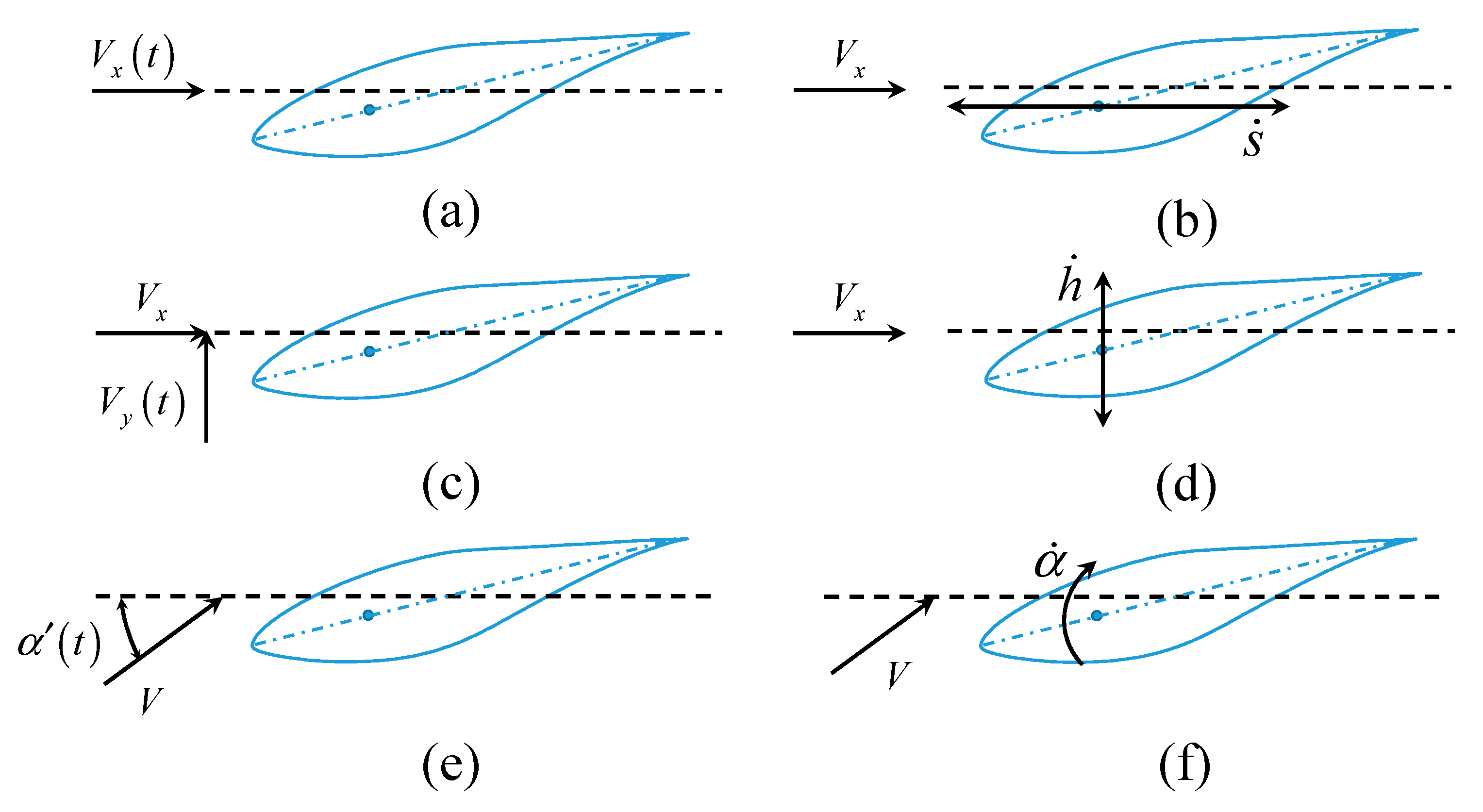
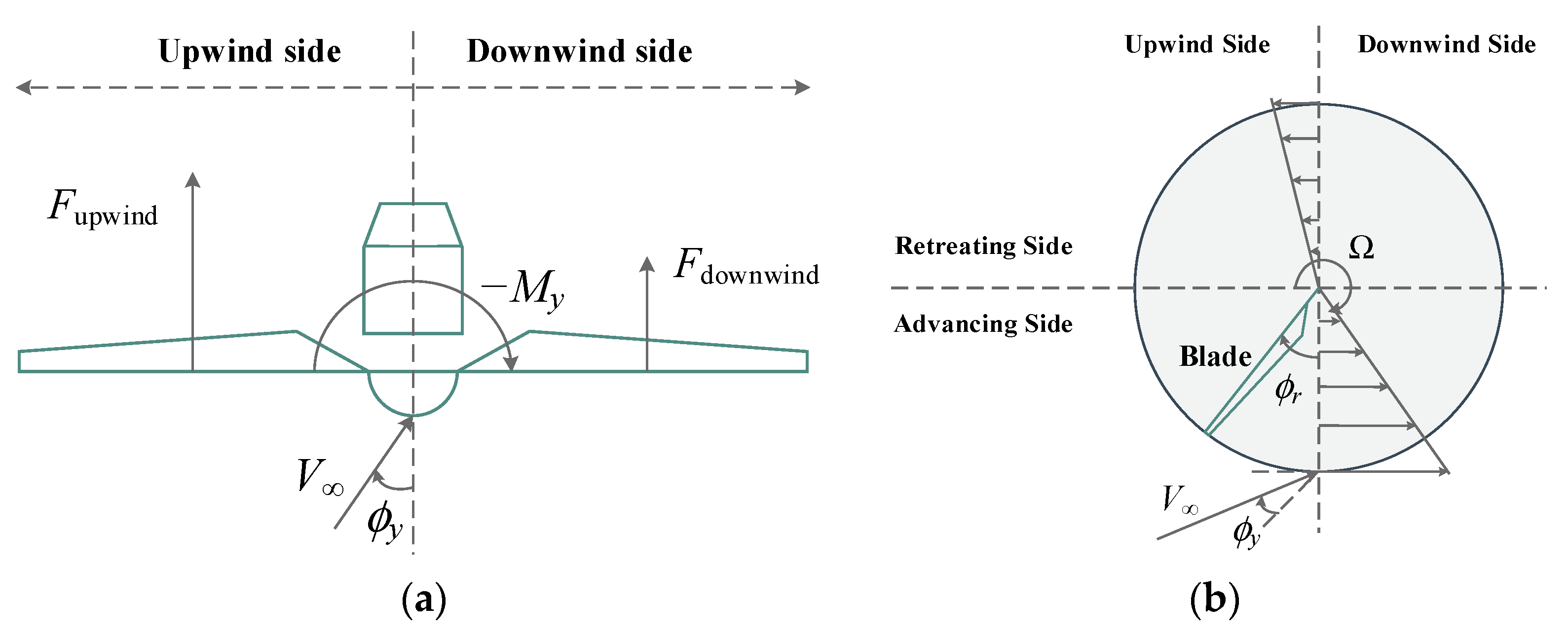
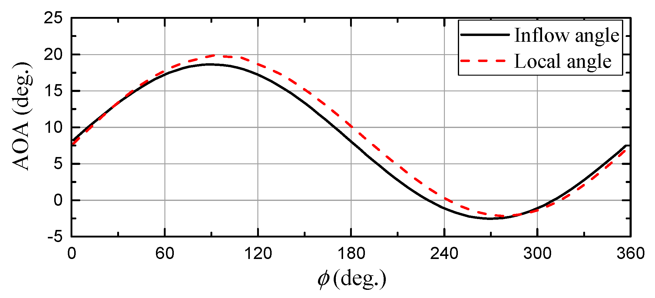
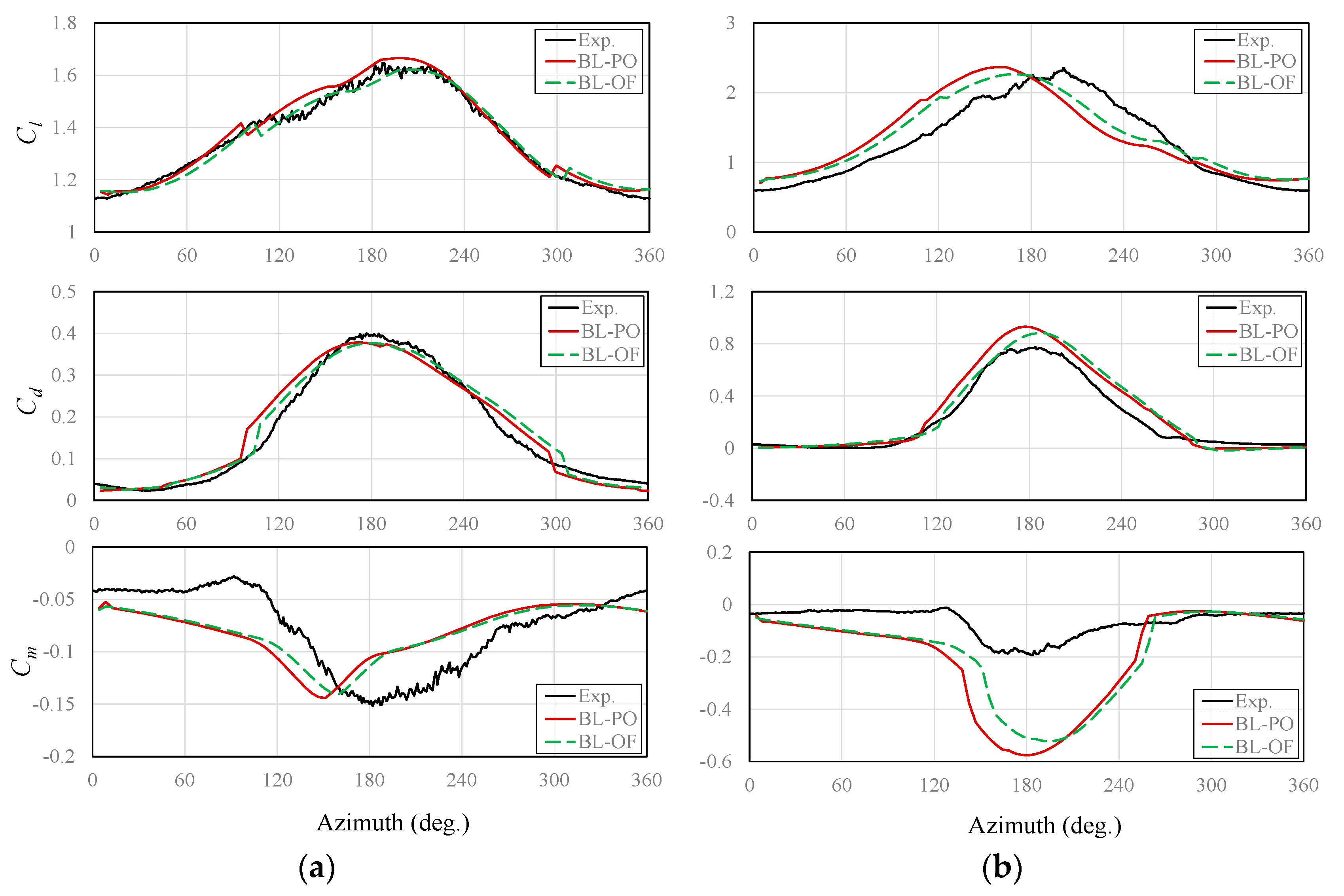
• Thirdly, a periodic AOA change (i.e., oscillating freestream, OF) results from the superposition of rotational velocity and the in-plane freestream velocity component (Figure 1e) under yawed inflow; as a counterpart, pitch oscillation (PO) occurs and affects the effective AOA under blade pitching or elastic bending (Figure 1f).

Van der Wall and Leishman [16] clarified the difference in the nature of the first pair, time-varying tangential velocity and fore-aft motion; the latter leads to a uniform perturbation velocity across the airfoil chord, while the former produces a perturbation velocity gradient across the chord. When the reduced frequency is low, both of them may be considered almost identical, which, however, is invalid for high reduced frequencies. Similarly, it can be speculated that time-varying freestream velocity will bring about a different effect on perturbation velocity from that of the plunging motion. For the third pair, Karbasian et al. [17] stated that OF can be referred to as PO. However, the equivalence relation between PO and OF still remains open from the point of view of Van der Wall and Leishman [16]. Practically, PO is generally used to conduct experimental studies and establish the engineering models. In order to improve the wind turbine unsteady aerodynamic prediction, it is necessary to clarify the relation between PO and OF.

To investigate the dynamic stall of the blade sections under PO and OF, the problem of dynamic stall must be considered as fully 3D due to the rotational effect [1]. During the last few decades, both dynamic stall and rotational effects have captured significant attention but have been studied independently. The rotational effects play an important role in the boundary layer development due to the centrifugal and Coriolis forces. The centrifugal force results in radial flow, thinning the boundary layer of the blade. On the other hand, the Coriolis force adds a chordwise positive pressure gradient, flattening the separated zone and delaying the flow separation. Because the gross output power and sectional lift are clearly elevated with flow separation delayed, the rotational effect is also called a rotational augmentation. Several stall delay models have been developed to correct the 2D airfoil data by Snel et al. [18], Chaviaropoulos and Hansen [19], Du and Selig [20], Raj [21], Bak et al. [22], Corrigan and Schillings [23], and Lindenburg [24]. Breton et al. [25] evaluated these existing models on the Phase VI rotor with a prescribed wake vortex code and discussed their deficiencies and strengths. The 3D rotational effect is relatively strong on small-scaled stall-controlled HAWTs, and almost all of the correction models are established on the studies of stall-controlled HAWT aerodynamics. However, Zahle et al. [26] and Bangga et al. [27] noted that rotational augmentation is still prominent in the root region of a 10 MW modern pitch-controlled HAWT. Bangga et al. [28] also observed the unsteady effects on rotational augmented blade loads under a turbulent inflow.

A comparative analysis of the dynamic stall under PO and OF on the NREL S809 airfoil [29] and the Phase VI rotor [30] is presented in this paper. Firstly, the quasi-steady thin-airfoil theory is used to clarify the difference between PO and OF in the induced perturbation velocity across the chord. Secondly, the unsteady RANS method is used to assess the equivalence relation between PO and OF. The turbulence is modeled by the SST k-ω eddy viscosity model [15] incorporated with the γ-Re_θ transition model [31]. Thirdly, the classical B-L model is used to predict the yawed response of the Phase VI rotor under PO and OF. Bak’s rotational stall delay model is incorporated into the dynamic stall model to consider rotational augmentation. The inverse BEM method is used to obtain the sectional AOAs and relative velocities from the experimental data. These extracted AOAs and velocities are then used to isolate the 3D rotational effect from the 3D unsteady aerodynamic data. All the predicted results agree well with the corresponding experimental data. It is found that PO and OF have an opposite effect on the effective airfoil camber. Therefore, it is necessary to separately consider the effects of PO and OF.

2. Methodology

The research objects are the Phase VI rotor and its basic airfoil, the NREL S809 airfoil. Here, PO denotes the sinusoidal pitch of the airfoil about the quarter-chord at a constant freestream velocity (Figure 1f), while OF denotes the sinusoidal change in the direction of inflow velocity at a constant magnitude to the stationary airfoil (Figure 1e). What is satisfied for both PO and OF is the same instantaneous angle between the freestream velocity and the chord as follows:

α(t) = α_m + Asin(2πft)

(1)

where α_m, A, and f are the mean AOA, the AOA amplitude, and the frequency of oscillation, respectively. The reduced frequency is often defined as k = πfc/V with V being the freestream velocity and c the chord length.

2.1. Thin-Airfoil Theoretical Analysis

Allowing for a simple analysis of the flow mechanism, the airfoil is simplified as a flat plate with its camber and thickness neglected here, and then, a quantitative comparison can be made with the quasi-steady thin-airfoil theory. The governing equation for thin-airfoil theory is Laplace’s equation. The idea is to place a vortex sheet singularity of unknown strength on the airfoil [32]. The strength of this vortex sheet is determined by satisfying the flow tangency on the camber line in conjunction with the Kutta condition at the trailing edge. Formulated in Fourier series, the general form of pressure distribution on the airfoil is as follows:

$$\Delta C_p\left(\alpha ,\theta \right)=4\left[A_0\left(\frac{1+\cos \theta }{\sin \theta }\right)+{\displaystyle \sum }_{n=1}^{\infty }{A}_n\sin n\theta \right]$$

(2)

where α is the AOA, and θ = cos⁻¹(1 − 2x/c) (x is the chordwise location with the leading edge denoted by x = 0). The coefficients A₀ and A_n are given by following equations:

$$\begin{gathered} A_0=\alpha -\frac{1}{\mathsf{\pi }}{{\displaystyle \int }}_0^{\mathsf{\pi }}\frac{\mathrm{d}y}{\mathrm{d}x}\mathrm{d}\theta \\ {A}_n=\frac{2}{\mathsf{\pi }}{{\displaystyle \int }}_0^{\mathsf{\pi }}\frac{\mathrm{d}y}{\mathrm{d}x}\cos n\theta \mathrm{d}\theta \end{gathered}$$

(3)

where y(x) describes the camber line of the airfoil. Integrating Equation (2) along the chord, we can obtain the lift coefficient, C_l = 2π(A₀ + 0.5A₁), and the pitching moment coefficient about the quarter-chord axis, C_m0.25 = −0.25π(A₁ − A₂). For PO, the pitch-rate term produces a linear variation in normal perturbation velocity [5], w(x) = −$\dot{\alpha }$(x − 0.25c) (where $\dot{\alpha }$ is the pitch rate and positive during upstroke) so that the induced camber is a parabolic arc (Figure 2). For OF, the normal perturbation velocity can be formulated as w(x) = Vα(t) − Vα(t−x/V). Because the quasi-steady condition means a low frequency, this formula can be linearized as w(x) = $\dot{\alpha }$x. Then, the term of dy/dx in Equation (3) can be replaced with w(x)/V. Hence, the lift coefficients are given by C_l = 2π(α + $\dot{\alpha }$c/2V) under PO and C_l = 2π(α − 3$\dot{\alpha }$c/4V) under OF, indicating an additional effective AOA, α_eq = $\dot{\alpha }$c/2V and α_eq = −3$\dot{\alpha }$c/4V, respectively.

In short, PO and OF have an opposite effect on the effective airfoil camber. During upstroke, PO increases the effective camber, while OF decreases the effective camber. During downstroke, PO decreases the effective camber, while OF increases the effective camber. Therefore, the lift under PO is higher during upstroke and lower during downstroke compared with the lift under OF. Notice that this effect is directly related to the pitch rate $\dot{\alpha }$ = 2πfAcos(2πft). Consequently, the difference between PO and OF is negligible at low variation frequencies and substantial at high ones.

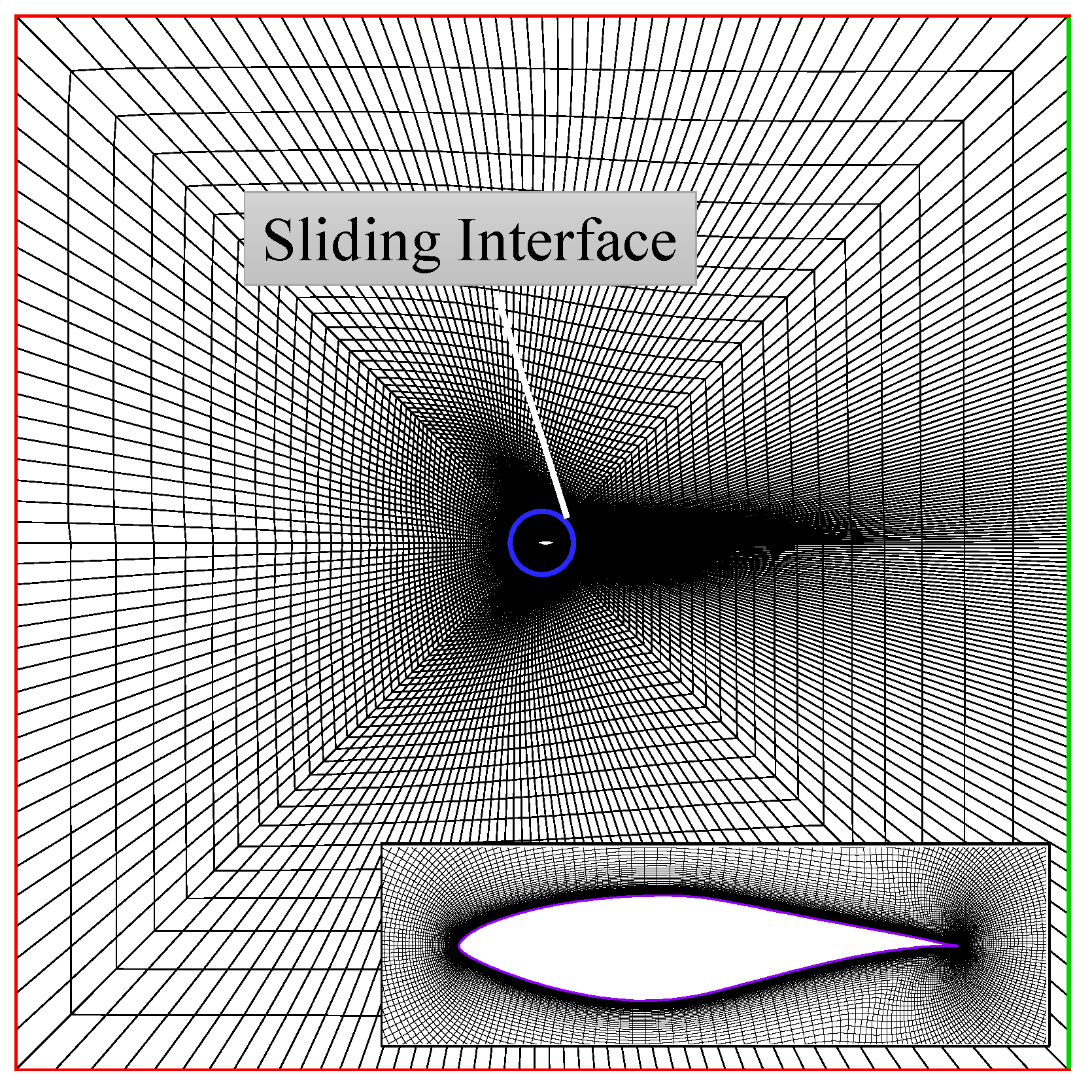
2.2. Numerical Modeling

For predictions of the dynamic stall, the commercial program ANSYS/FLUENT 16.0 (ANSYS, Inc., Canonsburg, PA, USA) [33] was used to solve the unsteady Reynolds-averaged Navier-Stokes equations. The mesh around airfoil geometry is generated in a structured O-type configuration to assure the wall orthogonality (Figure 3). The computational domain is exactly square. The first layer spacing off the wall is 10⁻⁵ c; this setting can ensure that the viscous sublayer is directly resolved with y⁺ less than 1. There are 48 normal layers in the boundary layer mesh, with the growth rate being 1.08. After a proper grid independence study, the total size of the computational mesh is set to be 51,090 with 245 wrap-around points and 206 normal layers. A far-field distance of 20 c away from the airfoil is sufficient. The left, upper, and lower sides are all inlet boundary with velocity imposed. The right side is outlet boundary with pressure imposed (Figure 3). To simulate the dynamic stall under PO, the sliding-mesh method [33] was used. Therefore, the computational zone was divided into two subdomains, a rotating region (inner) and a stationary region (outer). These two regions interact by a circular sliding interface; this control circle of the sliding interface is 1.2 c in radius (Figure 3). To simulate the dynamic stall under OF, a user-defined function was implemented on the velocity inlet boundaries. The typical Reynolds number of 1 × 10⁶ was selected in numerical simulations.

In order to obtain a good resolution, the third-order Monotone Upstream-Centered Schemes for Conservation Laws (MUSCL) convection scheme [33] is used for spatial discretization of the whole set of RANS and turbulence equations. This scheme was conceived of from the original MUSCL [34] by blending a central differencing scheme and a second-order upwind scheme. The second-order implicit scheme [33] is used for time differencing. Although it is theoretically valid that implicit methods are unconditionally stable with respect to the time step, nonlinearity effects would become prominent and oscillatory solutions may occur when the time step is increased. An operational cell convective courant number between 5 and 10 for viscous turbomachinery flows with an implicit scheme provides the best error damping properties [35]. On these bases, the number of inner iterations per time step is chosen to be 40 in this study to ensure the cell convective courant number is less than 10.

The pressure-based Coupled algorithm [33] is employed to handle the pressure-velocity coupling. Originally, the PISO algorithm [33] was preferable for transient problems, because it was derived from the SIMPLE algorithm [33] specifically for unsteady calculations. The PISO algorithm can yield accurate results with lower computational costs than the SIMPLE algorithm when time steps are sufficiently small. Both the SIMPLE and PISO algorithms, however, are known to converge slowly because the momentum equation and pressure-correction equation are solved separately. In the Coupled algorithm, the Navier-Stokes equations are directly solved through an implicit discretization of pressure in the momentum equations, with benefits in terms of robustness and convergence, especially with large time steps or with a poor-quality mesh. Balduzzi et al. [35] found that the obtained results with the Coupled algorithm are much closer to the experimental data than the SIMPLE and PISO algorithms. The lower sensitivity to the temporal discretization leads to the choice of the Coupled algorithm as the preferable and more robust formulation for the pressure-velocity coupling.

Because the incorporation of the transitional flow effects is a key element for an improved prediction of dynamic stall [14], the turbulence in the boundary layer is modeled by the four-equation SST k-ω eddy viscosity model [15] incorporated with the γ-Re_θ transition model [31].

2.3. Beddoes-Leishman Semi-Empirical Model

The classical B-L dynamic stall model [6] is capable of effectively assessing the unsteady loads with the flow physical features considered, and therefore, is fully implemented in the present work, including the leading-edge separation effect. Pereira et al. [10] have proven that it is unrealistic to disregard the leading-edge separation, because the wind turbine airfoils are thick. The main features and formulae of the B-L dynamic stall model may be summarized as follows.

2.3.1. Unsteady Attached Flow

Unsteady effects in attached flow conditions are simulated by the superposition of indicial aerodynamic responses for time step changes in the AOA. For a step change in the AOA, the normal force and pitching moment coefficients can be written as follows:

$$\begin{gathered} \Delta C_n=C_n^{\mathrm{c}}+C_n^{\mathrm{nc}} \\ \Delta C_m=C_m^{\mathrm{c}}+C_m^{\mathrm{nc}} \end{gathered}$$

(4)

where the superscripts c and nc denote the circulatory part and non-circulatory part of the aerodynamic loads, respectively. The indicial response can be approximated empirically in terms of the exponential function. Hence, the circulatory loading is as follows:

$$C_n^{\mathrm{c}}=C_{n\alpha }{\alpha }_{\mathrm{e}}^{\mathrm{c}}=C_{n\alpha }\left(\alpha \left(s\right)-X\left(s\right)-Y\left(s\right)\right)$$

(5)

where $C_{n\alpha }$ is the normal force slope, and the non-dimensional time s represents the distance travelled at the relative velocity by the airfoil in semi-chords; that is, s = 2Vt/c. X(s) and Y(s) are deficiency functions written in a special finite difference approximation to Duhamel’s integral as given by the following:

$$\begin{gathered} X\left(s\right)=X\left(s-\Delta s\right)\exp \left(-b_1\Delta s\right)+A_1\Delta \alpha \exp \left(-b_1\Delta s/2\right) \\ Y\left(s\right)=Y\left(s-\Delta s\right)\exp \left(-b_2\Delta s\right)+A_2\Delta \alpha \exp \left(-b_2\Delta s/2\right) \end{gathered}$$

(6)

Here, A₁, A₂, b₁, and b₂ are the coefficients of the indicial functions and are a function of the airfoil and the Mach number. Then, the circulatory pitching moment coefficient is given by the following:

$$C_m^{\mathrm{c}}=\left(0.25-x_{\mathrm{ac}}/c\right)C_n^{\mathrm{c}}$$

(7)

where x_ac is the position of the airfoil aerodynamic center measured from the leading edge. A similar recurrence relation is used for the non-circulatory part of the air loads, $C_n^{\mathrm{nc}}$ and $C_m^{\mathrm{nc}}$ (see [6] for details).

2.3.2. Unsteady Separated Flow

The non-linear effects of the trailing-edge separation are implemented using a Kirchhoff flow model. The movement of the unsteady flow separation point position is related to the static separation position via a deficiency function. The onset of the leading-edge separation, and hence the dynamic stall, is identified using a criterion based on the attainment of a critical local leading-edge pressure, which is further related to the normal force.

Under unsteady conditions, there is a lag in the leading-edge pressure with the increasing AOA, which can be expressed as a first-order lag as given by the following:

$$C_n^{\prime }=C_n^p-D_p$$

(8)

where

$$\begin{gathered} C_n^p=C_n^{\mathrm{c}}+C_n^{\mathrm{nc}} \\ {D}_p\left(s\right)=D_p\left(s-\Delta s\right)\exp \left(-\Delta s/T_p\right)+\left[C_n^p\left(s\right)-C_n^p\left(s-\Delta s\right)\right]\exp \left(-\Delta s/2T_p\right) \end{gathered}$$

(9)

The constant T_p can be determined empirically from unsteady airfoil data. The effective AOA ${\alpha }_f=C_n^{\prime }/C_{n\alpha }+{\alpha }_0$ after incorporating the unsteady pressure response is used to obtain the effective flow separation point $f^{\prime }$. In this study, $f^{\prime }$ is determined by look-up-table interpolation from the static airfoil data. The additional effects of a boundary layer response are considered as a first-order lag as given by the following:

$$f^{″}=f^{\prime }-D_f$$

(10)

where

$$D_f\left(s\right)=D_f\left(s-\Delta s\right)\exp \left(-\Delta s/T_f\right)+\left[f^{\prime }\left(s\right)-f^{\prime }\left(s-\Delta s\right)\right]\exp \left(-\Delta s/2T_f\right).$$

(11)

The constant T_f can be determined empirically from unsteady airfoil data. Then, the non-linear normal force coefficient is obtained by the Kirchhoff flow theory

$$C_n^f=C_{n\alpha }{\left(\frac{1+\sqrt{f^{″}}}{2}\right)}^2\left(\alpha -{\alpha }_0\right)$$

(12)

where ${\alpha }_0$ is the zero-lift AOA. Afterwards, the chordwise force coefficient is obtained by Gupa and Leishman’s approximation [11] as given by the following:

$$C_t^f=\{\begin{array}{cc}{C}_{n\alpha }\sqrt{f^{″}}\alpha \sin \alpha & C_n^{\prime }\le C_{n1}\\ K_1+C_{n\alpha }\sqrt{f^{″}}{f^{″}}^{\mathsf{\Phi }}\alpha \sin \alpha & C_n^{\prime }>C_{n1}\end{array}$$

(13)

where $C_{n1}$ is the critical normal force value and the leading-edge separation is initiated when $C_n^{\prime }>C_{n1}$. The parameter $K_1$ and $\mathsf{\Phi }$ are obtained from the static test data [11]. The pitching moment coefficient is obtained by fitting the ratio ${\mathrm{C}}_m/C_n$ in a least-square method from the static airfoil data as given by the following:

$$C_m^f=C_{m0}+\left[k_0+k_1\left(1-f^{″}\right)+k_2\sin \left(\mathsf{\pi }{f^{″}}^{\mu }\right)\right]C_n^f$$

(14)

where C_m0 is the zero-lift pitching moment coefficient. The values of k₀, k₁, k₂, and μ can be adjusted for different airfoils.

2.3.3. Vortex Force

The induced vortex force and the associated pitching moment are represented empirically in a time-dependent manner during dynamic stall. The total accumulated vortex normal force coefficient under unsteady conditions is given by the following:

$$C_n^v=C_n^v\left(s-\Delta s\right)\exp \left(-\Delta s/T_v\right)+\left[C_v\left(s\right)-C_v\left(s-\Delta s\right)\right]\exp \left(-\Delta s/2T_v\right)$$

(15)

where

$$C_v\left(s\right)=C_n^{\mathrm{c}}\left(s\right)\left[1+{\left(\frac{1+\sqrt{f^{″}}}{2}\right)}^2\right].$$

(16)

T_v is the vortex time decay constant. The center of pressure on the airfoil also varies with the chordwise position of the shedding vortex and will achieve a maximum value when the vortex reaches the trailing edge after a non-dimensional time period T_vl. A general representation of the center of pressure behavior (aft of the quarter-chord) is empirically formulated as follows:

$${\left(CP\right)}_v=0.25\left(1-\cos \frac{\mathsf{\pi }{T}_v}{T_{vl}}\right)$$

(17)

where T_v denotes the non-dimensional vortex time, $0\le T_v\le 2T_{vl}$ (i.e., $T_v=0$ at the onset of dynamic stall and $T_v=T_{vl}$ when the vortex reaches the trailing edge). Thus, the increment in the pitching moment about the quarter-chord due to dynamic stall is given by the following:

$$C_m^v=-{\left(CP\right)}_v·C_n^v.$$

(18)

The total unsteady air loads on the airfoil is then obtained by superposition as follows:

$$\begin{gathered} C_n=C_n^f+C_n^{\mathrm{nc}}+C_n^v \\ {C}_t=C_t^f+\left(C_n^{\mathrm{nc}}+C_n^v\right)\sin {\alpha }_{\mathrm{e}}^{\mathrm{c}} \\ {C}_m=C_m^{\mathrm{c}}+C_m^{\mathrm{nc}}+C_m^f+C_m^v \end{gathered}$$

(19)

Apart from dynamic stall, rotational augmentation is of crucial importance for wind turbine aerodynamic performance prediction. The rotational stall delay model of Bak et al. [22] is implemented. This model was developed on the difference in chordwise pressure distribution between the rotating blade section and the static airfoil. Although the obtained lift and drag coefficients were generally good, the modeled pitching moment coefficient indicated a poor agreement with the measurements, because the center of pressure was often underpredicted at large AOAs. Thus, a simple modification that the integrated location is changed from 0.25 to 0.1 was made to the pitching moment coefficient when fully separated flow occurs. Figure 4 implies an acceptable performance of this modification. It is generally acknowledged that the rotational augmentation is relatively apparent in separated flow; therefore, rotational augmentation mainly affects the nonlinear air loads.

To incorporate the rotational stall delay model into the dynamic stall model, the static airfoil data are corrected by Bak’s model firstly. Then, the static separation point is obtained from the Kirchhoff formulation (Equation (12)). The dynamic separation point is calculated by a first-order lag of the static separation point (Equation (10)), while the nonlinear normal force is reconstructed by Equation (12). Afterwards, the chordal force coefficient is obtained by Equation (13), with an increment added to consider the rotational augmentation. Finally, the nonlinear pitching moment coefficient is obtained by Equation (14), and a rotational increment is added as well. According to the recommendations of Pereira et al. [10] and Gupa et al. [11], the set of corresponding empirical time constants, T_p, T_f, T_v, T_vl, is as follows: 1.7, 8.0, 1.0, and 7.0, where T_p and T_f are related to the first-order lag of the leading-edge separation and trailing-edge separation, respectively, and both T_v and T_vl are the non-dimensional time constants related to the movement of the dynamic vortex.

The difference between PO and OF is addressed in the circulatory part of unsteady linear air loads, based on the thin-airfoil theory. To obtain input conditions, the sectional velocity components are extracted from the yawed measurements with the inverse BEM method [22,24,36,37,38]. This method has widely been used to determine the local AOA with the pre-determined local forces used to calculate the local induction factors and hence the induced velocities. In the inverse BEM method, Prandtl’s tip correction is used to consider the tip loss effect.

3. Results and Discussion

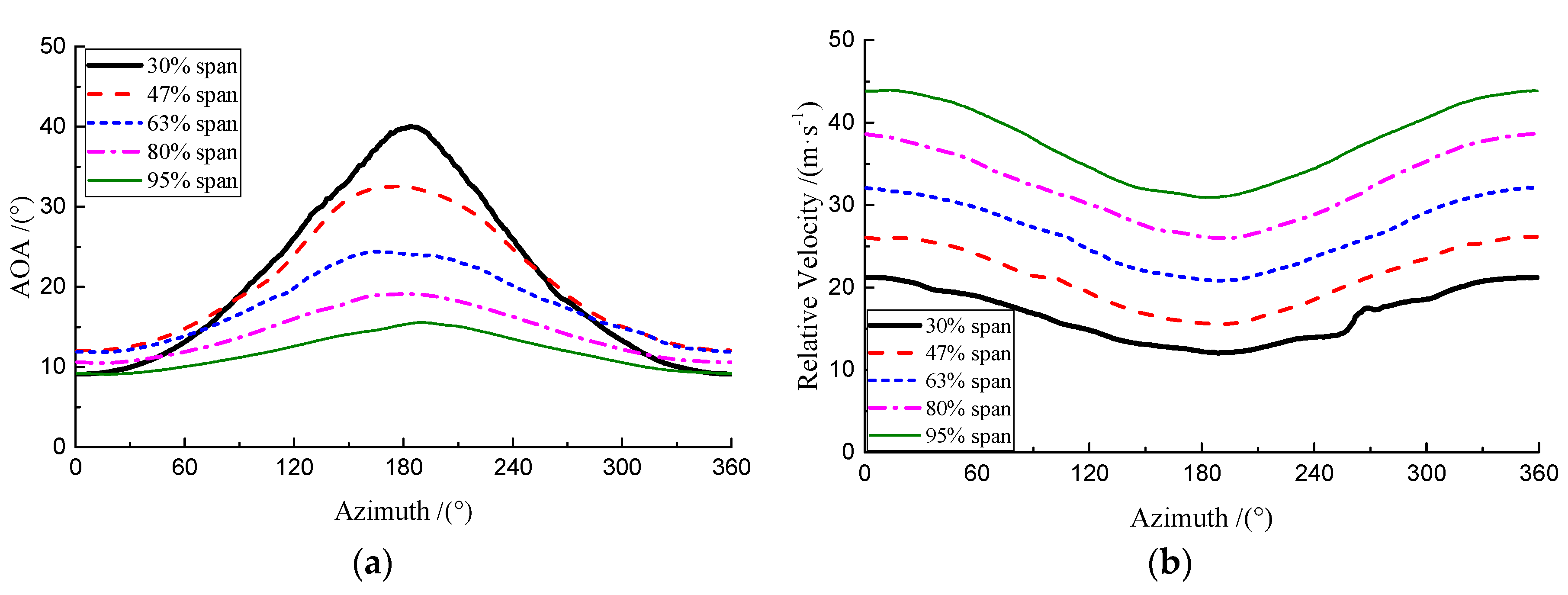
3.1. Time-Varying Sectional Incident Velocity under Yawed Inflow

Schepers [39] provided a detailed discussion on two aerodynamic effects under yawed inflow. One is the skewed wake effect, inducing an unbalanced axial velocity, producing asymmetric air loads, and then resulting in yawing stability. The other is the advancing and retreating blade effect, making the in-plane tangential velocity vary with the azimuth. Figure 5 provides the definitions of yaw angle and azimuth angle. Here, the blade azimuth is defined as zero at the 6-o’clock position, where the rotor is assumed to rotate clockwise. Figure 6 indicates the variations of the local AOA and relative velocity at different blade spanwise locations. These variations can be approximately formulated in trigonometric functions due to the rotational periodicity. It can be found that the spanwise location strongly influences the mean AOA and the AOA amplitude; the highest unsteadiness can be observed on the inboard blade despite a low velocity magnitude. Therefore, dynamic stall is often severe at inboard sections, where the rotational augmentation has manifested.

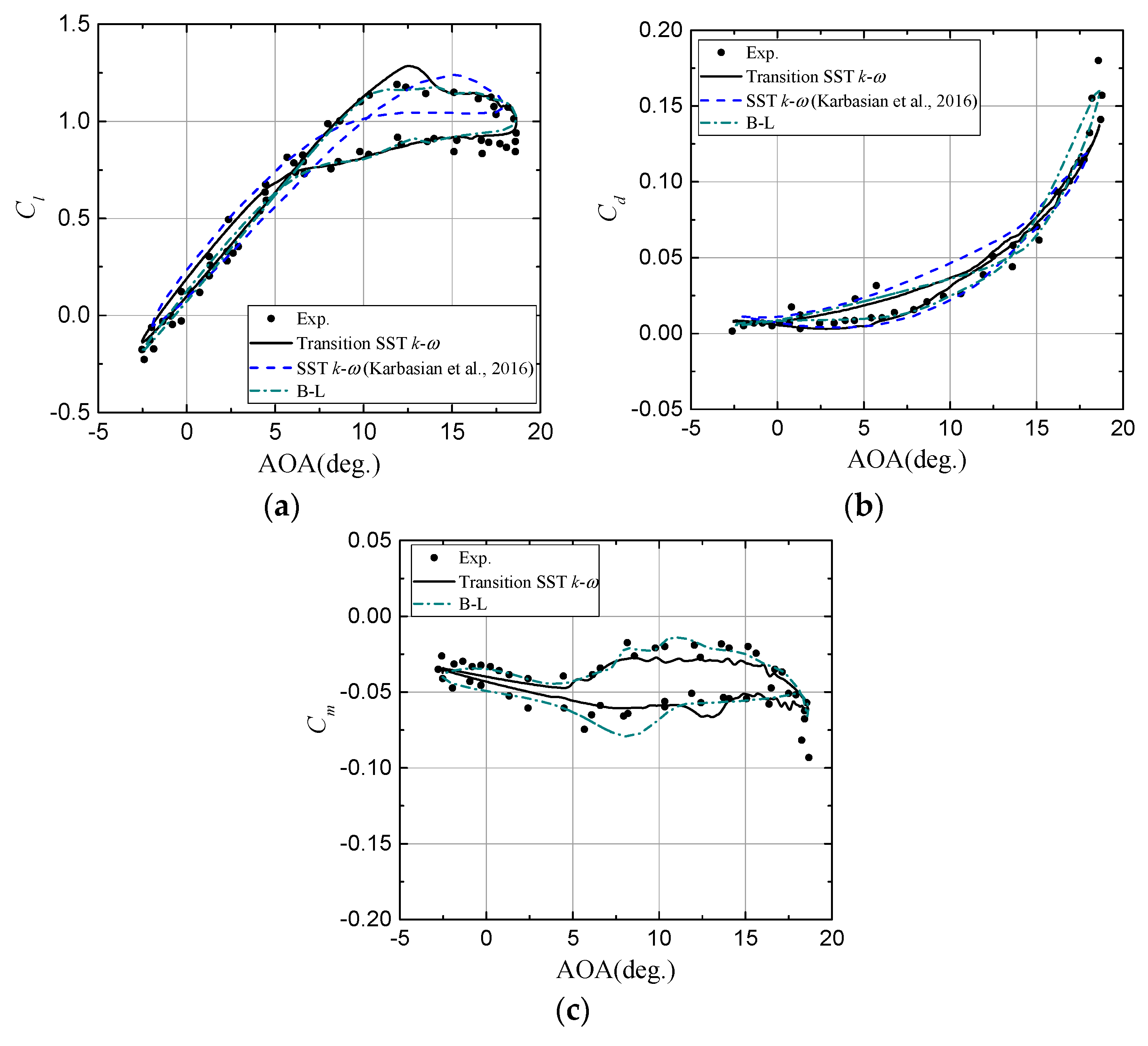
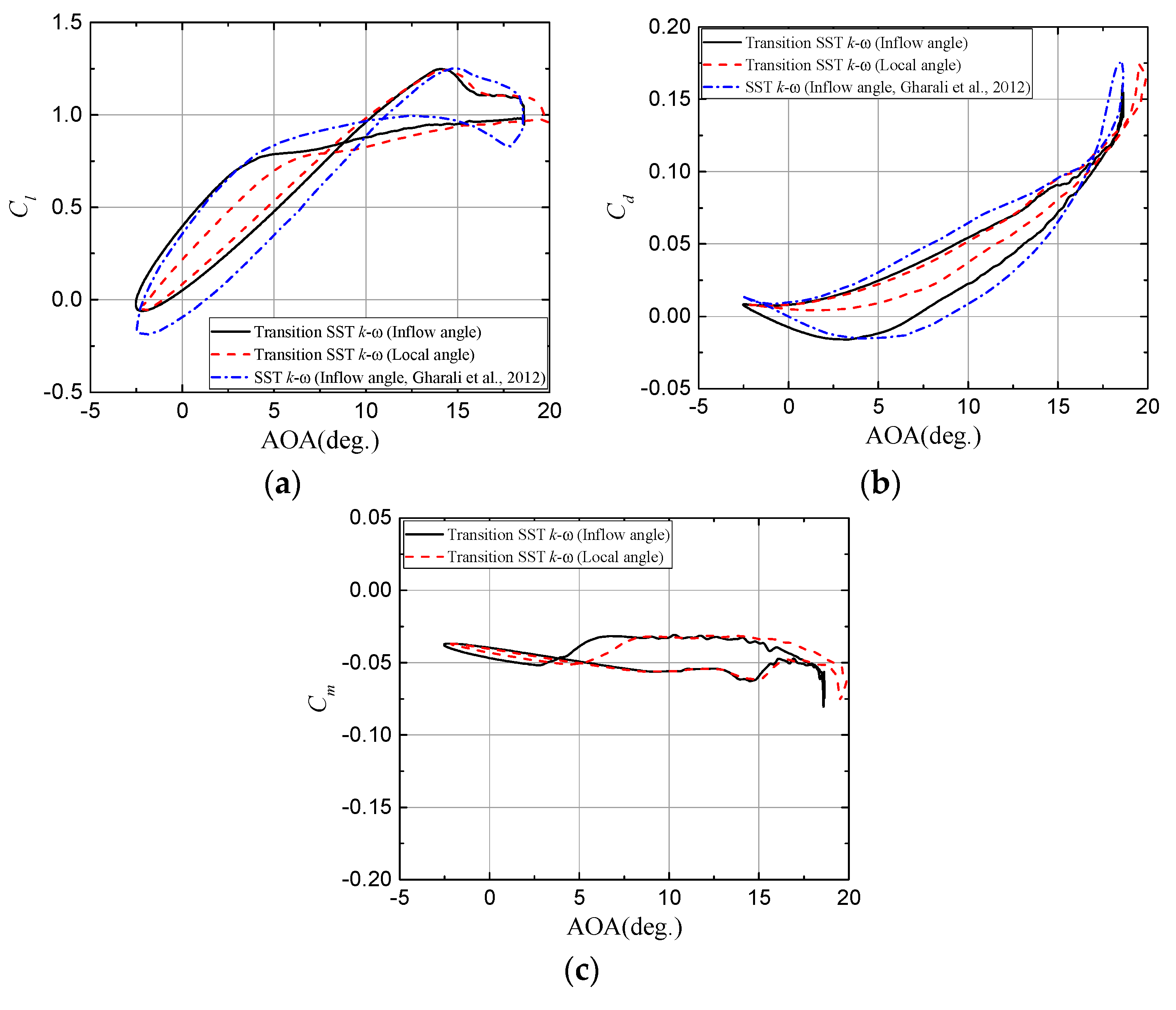
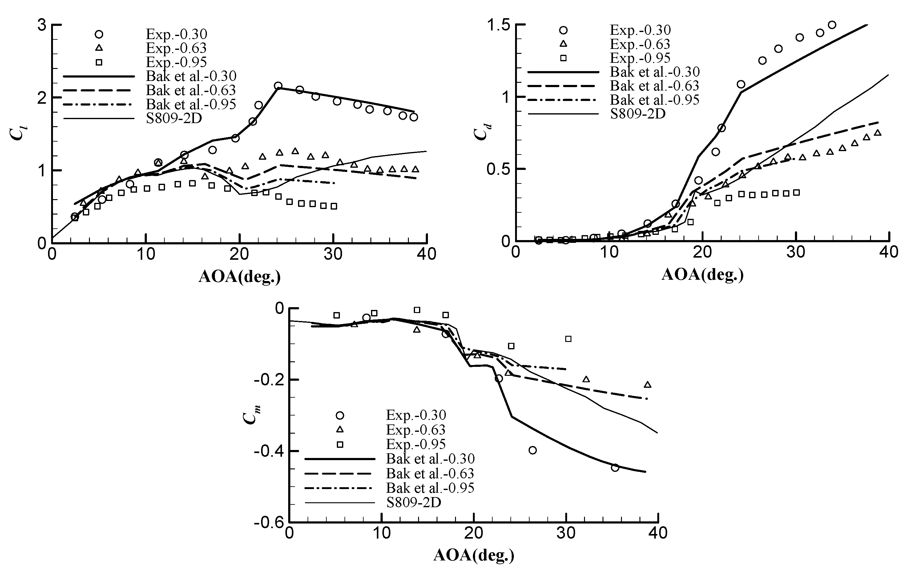
3.2. Validations of Numerical Modeling Methods

The pitch-oscillation case in the deep stall regime is selected for analyses of the grid independence and time step independence, where α_m = 14°, A = 10°, and k = 0.078. Different grid resolutions are obtained by changing the numbers of wrap-around points on the airfoil and normal layers; then, three types of grids are generated with total numbers of 37,850, 51,090, and 70,525, respectively. Three different time steps of 0.002 s, 0.001 s, and 0.0005 s are used with the steps per cycle being 273, 546, and 1092, respectively. However, there is no clear difference in the lift coefficient among the test cases. The streamwise velocity profile is used to estimate the capability of capturing flow structures; this velocity profile is at mid-chord at the phase angle of 90° (i.e., φ = 90°, where φ = 2πft). The coarsen grid and large time step can yield clear deviation (Figure 7). Finally, the grid in the size of 51,090 and the time step of 0.001 s are chosen as the computational settings.

In light stall, the numerical results agree well with the experimental data [40] as shown in Figure 8. An improvement over Karbasian, Esfahani, and Barati’s CFD results [17] can be observed due to the consideration of the transition effect. The B-L model shows a reasonable representation of unsteady aerodynamics. Because of a lack of measurements under OF, the CFD results are compared with those of Gharali et al. in the same conditions [41]. First and foremost, it is necessary to clarify the determination of the AOA under OF. In steady flow, the AOA is defined as the angle between the chord and freestream velocity, and this instantaneous AOA (denoted as ‘inflow angle’) is assured at same value for both motions in the computations. Actually, the true AOA (denoted as ‘local angle’) is different, because the relative velocity direction to the airfoil can be influenced by the freestream time lag and flow disturbance of the airfoil. To obtain the local angle and compare it with the inflow angle, we extract the unsteady relative velocity vector at the location of 3 c before the airfoil stagnation point (Figure 9). An apparent lag between the two types of AOAs can be observed during downstroke. The variation amplitude of the local angle becomes slightly larger. Both the trend and the shape of the hysteresis loop agree well with the results of Gharali et al. [41], as shown in Figure 10. A notable feature is that the hysteresis loop is more apparent with respect to the inflow angle than to the local angle. To avoid ambiguity, the phase angle will replace the AOA as an independent variable afterwards.

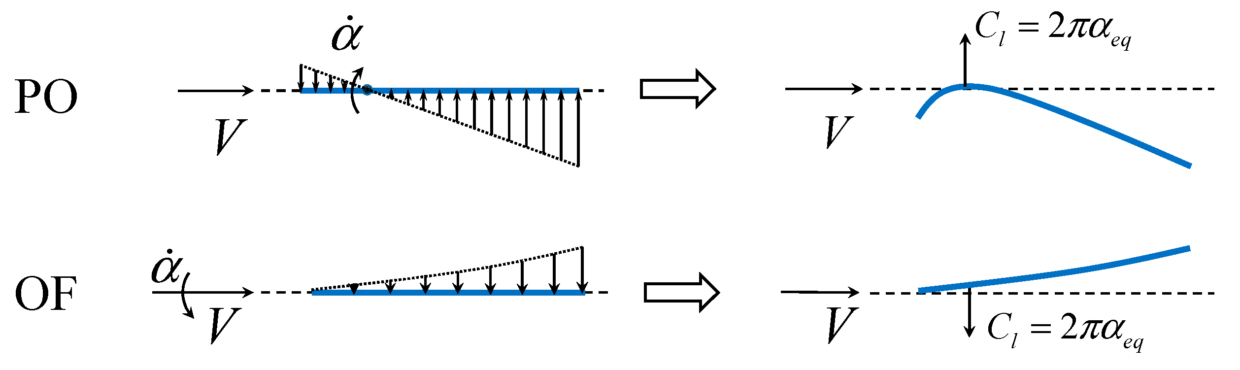
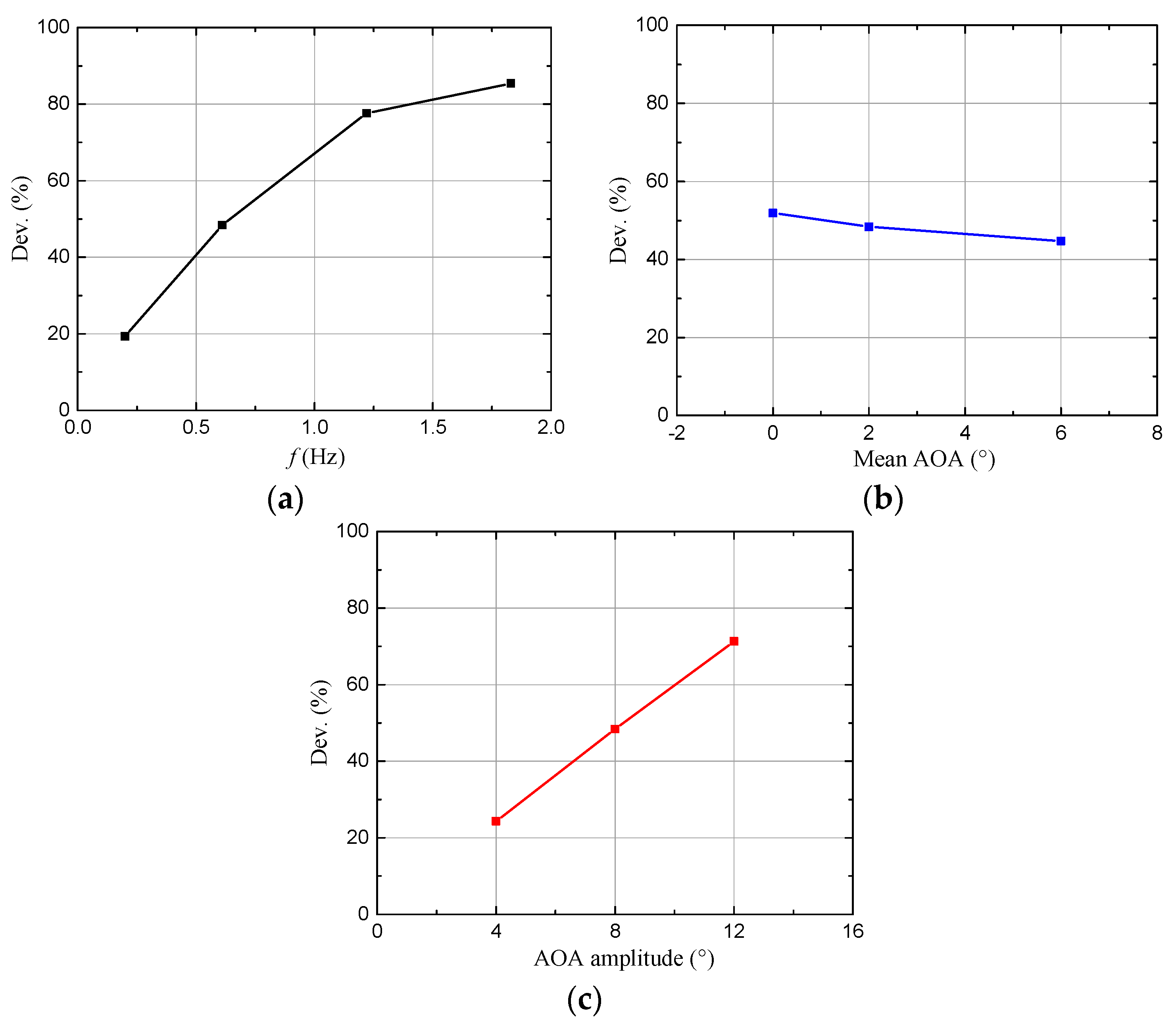
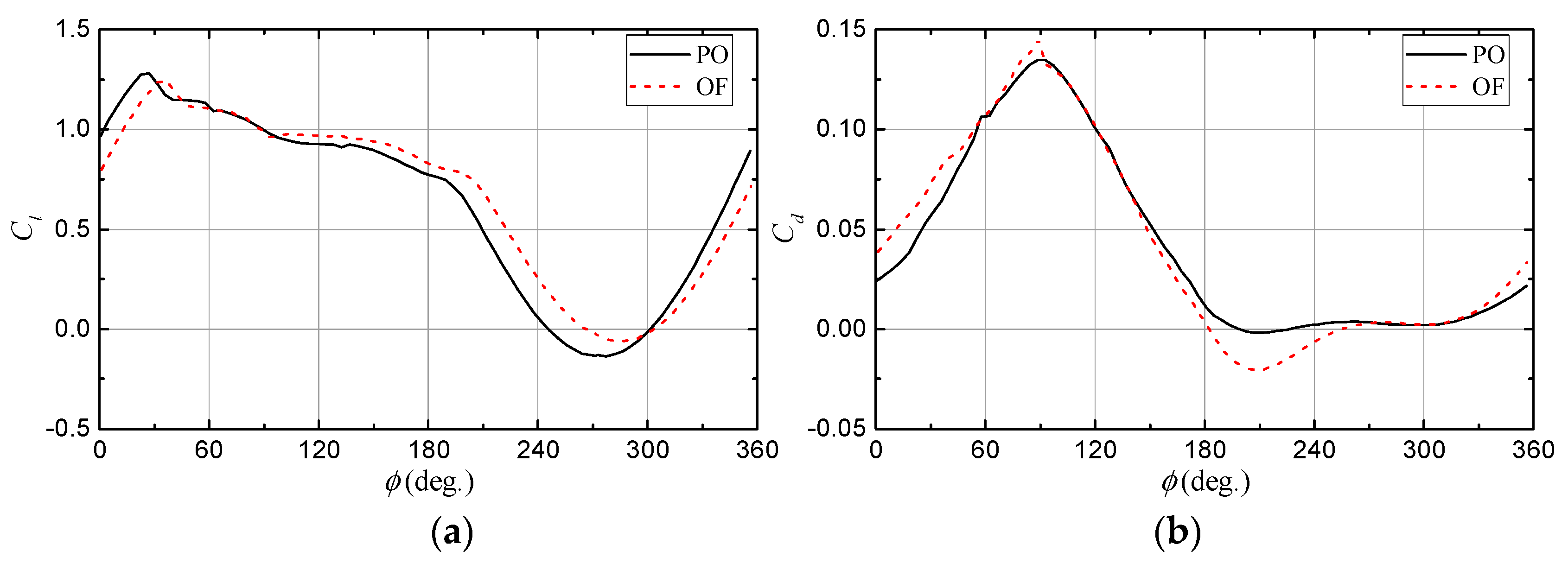
3.3. Equivalence Analysis between Pitch Oscillation and Oscillating Freestream

The aforementioned theoretical analysis indicates an opposite effect of PO and OF on the effective airfoil camber. Figure 11 shows the variations of the lift and the drag coefficients along one cycle. Notice that the difference in the nonlinear air loads (where φ is from 30° to 180°) is relatively negligible. A clear difference in the linear lift coefficient can be observed with a higher value under PO during upstroke and a higher value under OF during downstroke; the CFD results agree well with the thin-airfoil theory. From the vorticity contours in Figure 12, flow is attached to the airfoil and there is no obvious difference between the two motions from φ = 270° to φ = 360°. When the AOA reaches the maximum at φ = 90°, the flow separation is apparent under both PO and OF. The separated flow under PO is more persistent. In contrast, the vortex under OF rolls up and then sheds into wake. Despite a great difference in separated flow structure between the two motions, the associated aerodynamic loads do not show great differences. The possible reason is that the pressure distribution under PO possesses a sharp leading-edge suction peak, while the pressure distribution under OF experiences an elevated pressure on the suction side due to the separated vortex. These two factors may lead to an almost equal value in calculation. Figure 13 shows the unsteady pressure variations at different chordwise locations at α_m = 2°, A = 8°, and k = 0.078. It is obvious that there is a stronger suction peak under PO than under OF. However, the pressure coefficient under OF decreases with a time lag.

Because the difference between the two motions focuses on the linear part of the aerodynamic loads, the unsteady aerodynamic effect only at the low AOA is assessed. The mean AOA, AOA amplitude, and oscillation frequency are chosen as parameters to evaluate the difference. The deviation of the normal coefficient along one cycle between the two motions is defined as follows:

$$Dev.=\frac{max\left(\left|C_{n,PO}(\varnothing )-C_{n,OF}(\varnothing )\right|\right)}{C_{n,qs}}$$

(20)

where C_n,qs is the quasi-steady normal coefficient at the mean AOA. Figure 14 indicates that the oscillation frequency f and the AOA amplitude A affect the deviation more strongly than the mean AOA. From the thin-airfoil theory, the key is the pitch rate $\dot{\alpha }$ = 2πfAcos(2πft). Because f and A are factors of the pitch rate, the deviation becomes great when f and A are high. Under yawed inflow, the oscillation frequency is directly determined by the rotor speed, and the AOA amplitude is seriously affected by the yaw angle. Consequently, it is necessary to consider the effects of PO and OF separately.

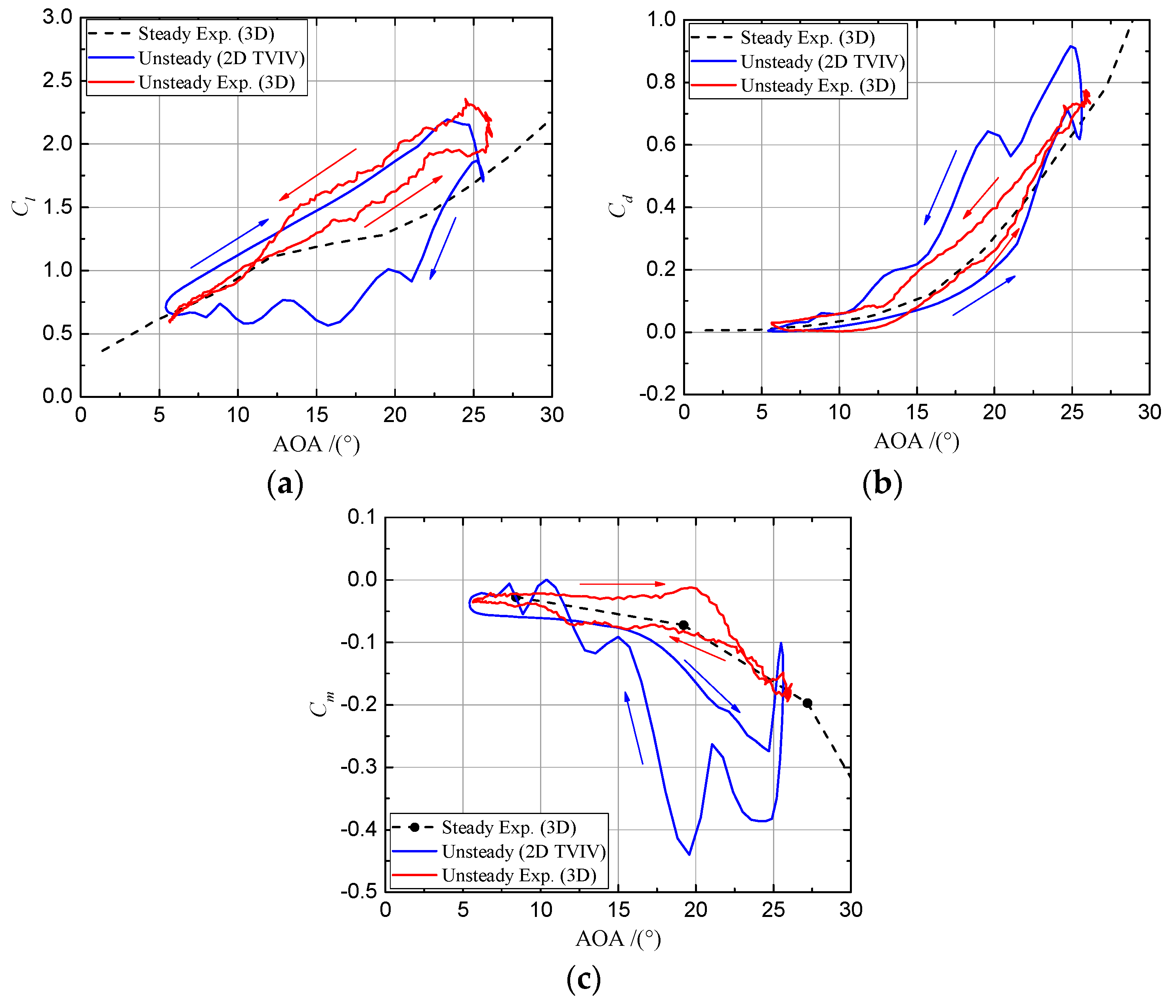
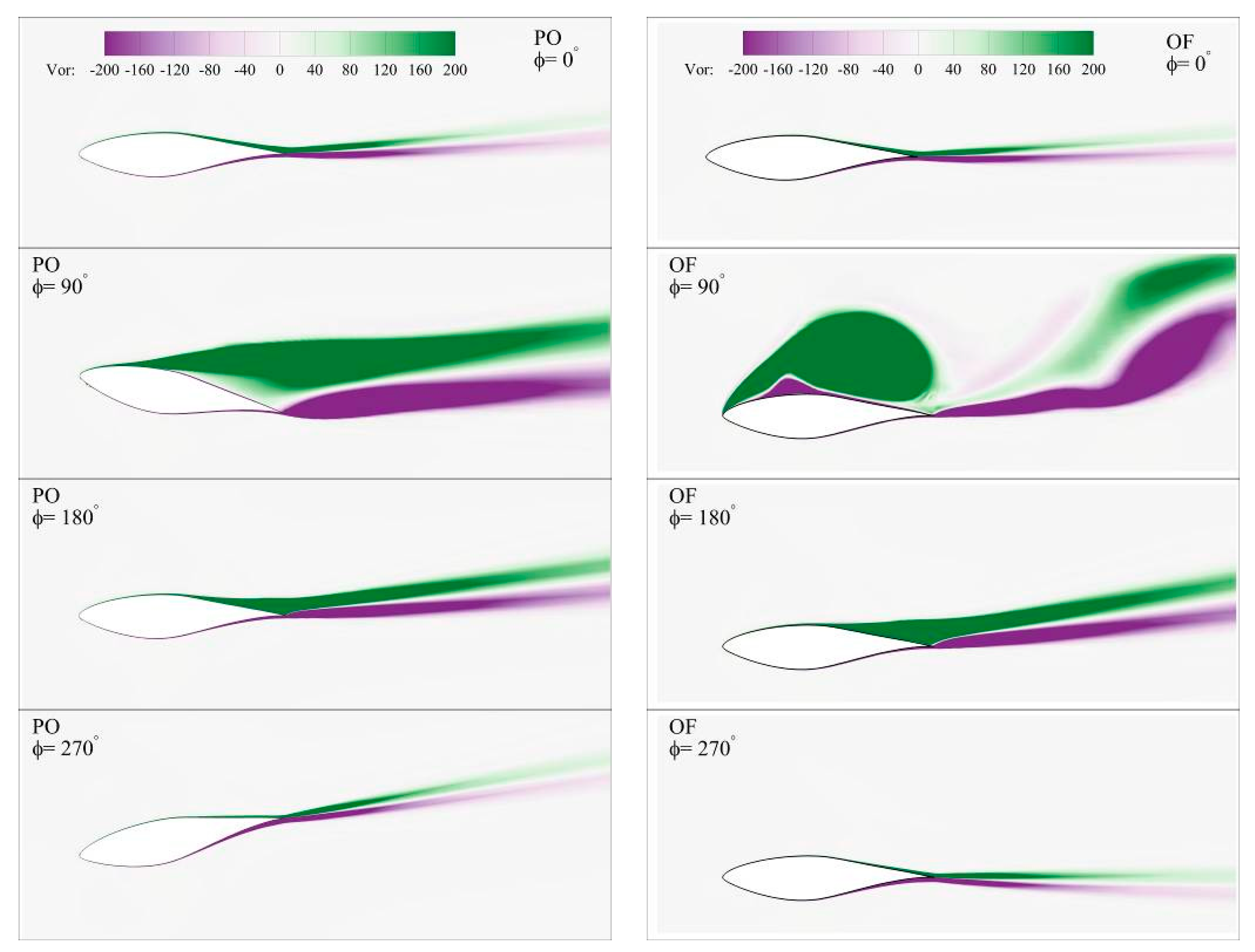
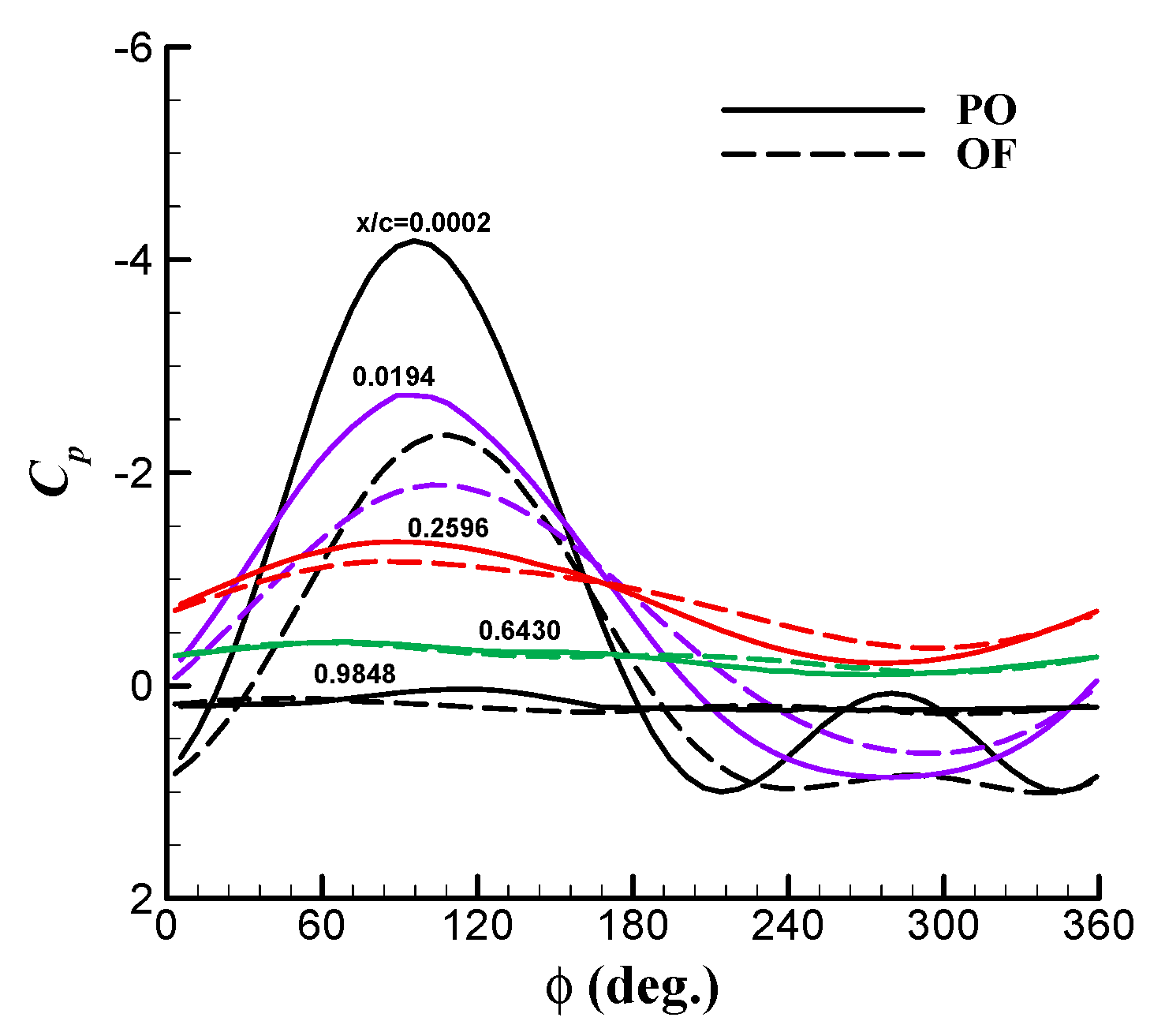
3.4. Comparison of Dynamic Stall in Yawed Condition between the Two Motions

The 30% span of the Phase VI blade is investigated due to the manifest dynamic stall on the inboard blade. The wind speed is 10 m/s, and the yaw angle is 10° and 30°, respectively (the cases of S1000100 and S1000300 in NREL UAE Phase VI [30]). The B-L dynamic stall model incorporated with Bak’s rotational stall delay model shows a good agreement with the experimental data for the yaw angle of 10°, as shown in Figure 15. A noticeable difference in both the lift coefficient and drag coefficient between the 2D and 3D results is observed, manifesting the 3D rotational effect.

Figure 16 shows the aerodynamic force coefficients and pitching moment coefficient varying with azimuthal angle at the yaw angles of 10° and 30°, respectively. The calculated results are generally in a good agreement with the experimental data. When the yaw angle increases, the 3D dynamic stall becomes more intense with the high lift coefficient, but trends of air load variations are consistent. The difference between PO and OF is moderate. As aforementioned, in 2D cases, the aerodynamic coefficients under PO are higher during upstroke and lower during downstroke. A slight improvement can be observed in the prediction under OF; the possible reason is that dynamic stall under yawed inflow is essentially a velocity-varying problem without pitch motion and fore–aft motion. Notice that prediction of the pitching moment coefficients is quite poor in both amplitudes and trends. Given that the pitching moment depends not merely on the integrated normal force but also on the location of the center of pressure, it is somewhat not surprising that the predicted pitching moment is unsatisfactory under the dynamic condition, because 3D effects have an influence on the normal force and on the movement of the center of pressure, which depends on appropriate coupling of the dynamic stall and the 3D rotational stall delay models. This problem may be solved only if deep understanding and accurate modeling of both the dynamic stall and the 3D stall delay are achieved. Nevertheless, the results from the B-L dynamic stall model show a different effect between PO and OF when their different additional camber effects are included.

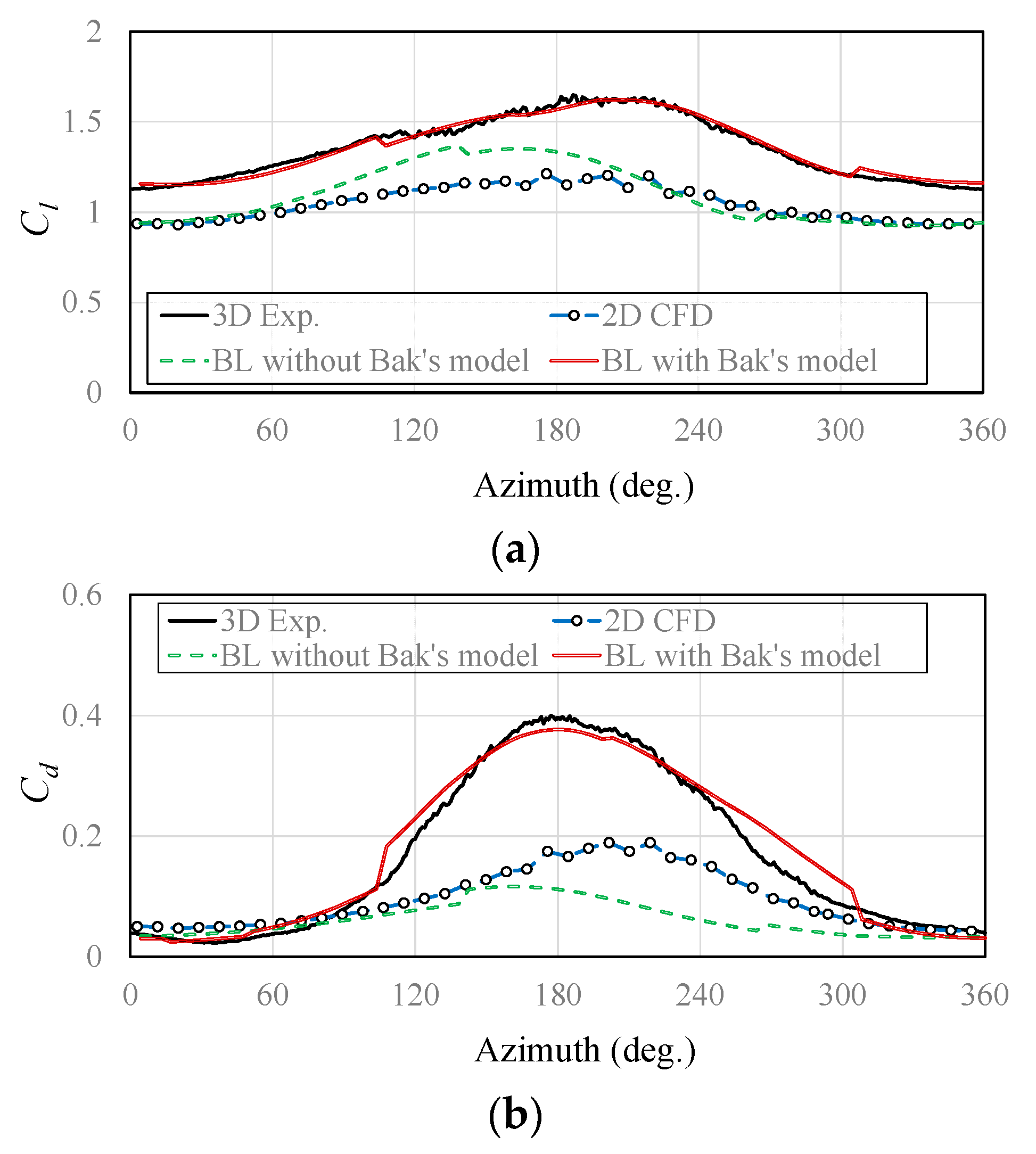
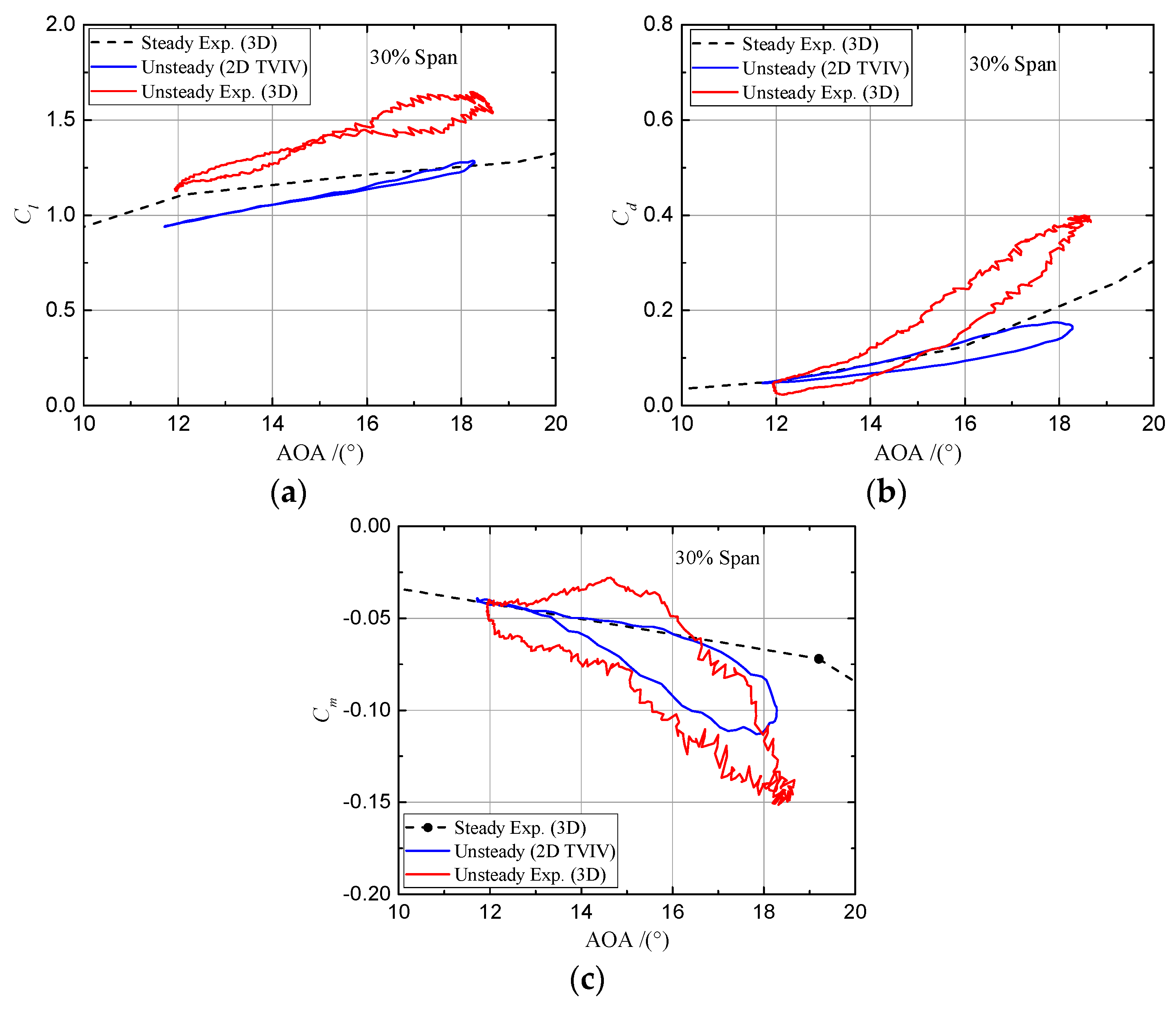
3.5. Effect of Rotational Augmentation on the Dynamic Stall of the Inboard Blade

Because the rotational effect greatly suppresses the flow separation, the lift and nose-down pitching moment coefficients are increased. However, it is unclear whether the rotational stall delay effect under steady conditions is consistent with its performance under unsteady conditions. To provide an insight into the coupled effect of the rotational augmentation and dynamic stall, an extended analysis is conducted. As rotational augmentation is often isolated by making comparisons between 2D flow and 3D rotational flow [42], our strategy is to isolate the rotational augmentation by comparing the CFD results under an equivalent planer motion with yawed experimental data; the former contains only dynamic stall and the latter is coupled with rotational augmentation. The equivalent planer motion of a rotating blade section is obtained by the 2D time-varying incident velocity (2D TVIV, Figure 1a,c), including variations of the sectional AOA and the relative velocity magnitude.

Figure 17 shows the hysteresis loops of the aerodynamic coefficients at the 30% span. Because both the mean AOA and the AOA amplitude are low, the aerodynamic forces are generally attached to the unsteady linear part with almost no stall. Rotational augmentation apparently elevates the lift and drag coefficients, as under steady conditions. The value is even higher than the steady experimental data under axial inflow, meaning that the separation is more delayed in 3D rotational unsteady flow than in 3D rotational steady flow. Hence, both rotational augmentation and unsteady effects lead to a delayed flow separation and the elevated lift coefficient at a low yaw angle.

When the yaw angle is high, the air load variation is more severe with the large AOA amplitude. In comparison with Figure 17, Figure 18 shows hysteresis loops of the aerodynamic coefficients at 30° yaw angle at 30% span. It is rather remarkable that the 2D and 3D hysteresis loops of the lift coefficient are in the opposite direction. The 3D lift coefficient is even lower than the 2D value with the AOA increasing, meaning no rotational augmentation effect in the lift force. However, when the AOA decreases, the rotational augmentation dramatically advances the reattachment and results in a flattened hysteresis loop in an anticlockwise direction. In other words, the rotational augmentation effectively pushes the reattachment point rearward and reduces the hysteresis of the air loads on the downwind side (where the AOA is decreasing) (Figure 5b). Because of the unsteady effects, the unsteady 3D experimental data shows an apparent increase in the lift coefficient over the steady 3D experimental data. However, the 3D drag and pitching moment coefficients slightly vary around the steady data. With the AOA decreasing, the hysteresis loop under 2D TVIV indicates a notable additional fluctuation from secondary vortices in the pitching moment coefficient. In short, at a high yaw angle, the rotational augmentation is minor on the upwind side and effectively reduces the hysteresis on the downwind side, while unsteady effects greatly delay the flow separation and elevate the lift coefficient along the whole cycle.

4. Conclusions

Dynamic stall is very common on HAWTs, resulting from many aerodynamic sources. Dynamic stall plays an important role in unsteady air loads. The accurate prediction of dynamic stall is extremely important for structural analysis. This study provides a comparative analysis of dynamic stall under pitch oscillation (PO) and oscillating freestream (OF) on wind turbine airfoil and blade, using the quasi-steady thin-airfoil theory, CFD method, and Beddoes-Leishman dynamic stall engineering model.

From the quasi-steady thin-airfoil theory, PO and OF have an opposite effect on the effective airfoil camber and the associated lift coefficient. The CFD results show that the difference between PO and OF mainly exists in the linear part of the aerodynamic loads. The deviation between these two motions is greatly influenced by the reduced frequency and the AOA amplitude. For the yawed response predictions, the Beddoes-Leishman dynamic stall model coupled with a rotational stall delay model also show a different effect between PO and OF. In addition, the effect of the rotational augmentation on the unsteady air loads is assessed. At a low yaw angle, the rotational augmentation apparently elevated the lift and drag coefficients along the whole cycle, as under steady conditions. At a high yaw angle, however, the rotational augmentation apparently flattens the hysteresis loop and its effect during which the AOA dynamically decreasing is more obvious than when the AOA is dynamically increasing.

It may be concluded from this work that dynamic stall behaviors under PO and OF are different at certain conditions and should separately be modeled in engineering.

References

1. Leishman, J.G. Challenges in modelling the unsteady aerodynamics of wind turbines. Wind Energy 2002, 5, 85–132. [Google Scholar] [CrossRef] [Green Version]
2. McCroskey, W.J. The Phenomenon of Dynamic Stall; National Aeronautics and Space Administration: Washington, DC, USA, 1981. [Google Scholar]
3. Carr, L.W. Progress in analysis and prediction of dynamic stall. J. Aircr. 1988, 25, 6–17. [Google Scholar] [CrossRef]
4. Butterfield, C.P. Aerodynamic pressure and flow-visualization measurement from a rotating wind turbine blade. In Proceedings of the Eighth ASME Wind Energy Symposium, Houston, TX, USA, 22–25 January 1989; pp. 245–256. [Google Scholar]
5. Leishman, J.G. Principles of Helicopter Aerodynamics, 2nd ed.; Cambridge University Press: Cambridge, UK, 2006. [Google Scholar]
6. Leishman, J.G.; Beddoes, T.S. A Semi-Empirical Model for Dynamic Stall. J. Am. Helicopter Soc. 1989, 34, 3–17. [Google Scholar] [CrossRef]
7. Tran, C.T.; Petot, D. Semi-empirical model for the dynamic stall of airfoils in view of the application to the calculation of responses of a helicopter blade in forward flight. Vertica 1981, 5, 35–53. [Google Scholar]
8. Øye, S. Dynamic Stall Simulated as Time Lag of Separation; Technical University of Denmark: Lyngby, Denmark, 1991. [Google Scholar]
9. Hansen, M.H.; Gaunaa, M.; Madsen, H.A. A Beddoes-Leishman Type Dynamic Stall Model in State-Space and Indicial Formulation; Risø National laboratory: Roskilde, Denmark, 2004. [Google Scholar]
10. Pereira, R.; Schepers, G.; Pavel, M.D. Validation of the Beddoes-Leishman dynamic stall model for horizontal axis wind turbines using MEXICO data. Wind Energy 2013, 16, 207–219. [Google Scholar] [CrossRef]
11. Gupta, S.; Leishman, J.G. Dynamic stall modelling of the S809 aerofoil and comparison with experiments. Wind Energy 2006, 9, 521–547. [Google Scholar] [CrossRef]
12. Johansen, J. Unsteady Airfoil Flows with Application to Aeroelastic Stability; Risø National laboratory: Roskilde, Denmark, 1999. [Google Scholar]
13. Visbal, M.R. Numerical Investigation of Deep Dynamic Stall of a Plunging Airfoil. AIAA J. 2011, 49, 2152–2170. [Google Scholar] [CrossRef]
14. Ekaterinaris, J.A.; Platzer, M.F. Computational prediction of airfoil dynamic stall. Prog. Aeosp. Sci. 1998, 33, 759–846. [Google Scholar] [CrossRef] [Green Version]
15. Menter, F.R. Two-Equation Eddy-Viscosity Transport Turbulence Model for Engineering Applications. AIAA J. 1994, 32, 1598–1605. [Google Scholar] [CrossRef]
16. Van der Wall, B.G.; Leishman, J.G. On the Influence of Time-Varying Flow Velocity on Unsteady Aerodynamics. J. Am. Helicopter Soc. 1994, 39, 25–36. [Google Scholar] [CrossRef]
17. Karbasian, H.R.; Esfahani, J.A.; Barati, E. Effect of acceleration on dynamic stall of airfoil in unsteady operating conditions. Wind Energy 2016, 19, 17–33. [Google Scholar] [CrossRef]
18. Snel, H.; Houwink, R.; Bosschers, J. Sectional Prediction of Lift Coefficients on Rotating Wind Turbine Blades in Stall; Energy Research Center of the Netherlands: Petten, The Netherlands, 1993. [Google Scholar]
19. Chaviaropoulos, P.K.; Hansen, M.O.L. Investigating three-dimensional and rotational effects on wind turbine blades by means of a quasi-3D Navier-Stokes solver. J. Fluids Eng. Trans. ASME 2000, 122, 330–336. [Google Scholar] [CrossRef]
20. Du, Z.; Selig, M. A 3-D stall-delay model for horizontal axis wind turbine performance prediction. In Proceedings of the 36th AIAA Aerospace Sciences Meeting and Exhibit, 1998 ASME Wind Energy Symposium, Reno, NV, USA, 12–15 January 1998. [Google Scholar]
21. Raj, N.V. An Improved Semi-Empirical Model for 3-D Post-Stall Effects in Horizontal Axis Wind Turbines; University of Illinois: Urbana-Champaign, IL, USA, 2000. [Google Scholar]
22. Bak, C.; Johansen, J.; Andersen, P.B. Three-Dimensional Corrections of Airfoil Characteristics Based on Pressure Distributions. In Proceedings of the European Wind Energy Conference and Exhibition (EWEC), Athens, Greece, 27 February–2 March 2006. [Google Scholar]
23. Corrigan, J.J.; Schillings, J.J. Emprical Model for Stall Delay Due to Rotation. In Proceedings of the American Helicopter Society Aeromechanics Specialists Conference, San Francisco, CA, USA, 19–21 January 1994. [Google Scholar]
24. Lindenburg, C. Investigation into Rotor Blade Aerodynamics; Energy research Centre of the Netherlands Petten: Petten, The Netherlands, 2003. [Google Scholar]
25. Breton, S.P.; Coton, F.N.; Moe, G. A Study on Rotational Effects and Different Stall Delay Models Using i a Prescribed Wake Vortex Scheme and NREL Phase VI Experiment Data. Wind Energy 2008, 11, 459–482. [Google Scholar] [CrossRef]
26. Zahle, F.; Bak, C.; Guntur, S.; Soslashrensen, N.N.; Troldborg, N. Comprehensive aerodynamic analysis of a 10 MW wind turbine rotor using 3D CFD. In Proceedings of the 32nd ASME Wind Energy Symposium, National Harbor, MD, USA, 13–17 January 2014; p. 15. [Google Scholar]
27. Bangga, G.; Lutz, T.; Jost, E.; Kramer, E. CFD studies on rotational augmentation at the inboard sections of a 10 MW wind turbine rotor. J. Renew. Sustain. Energy 2017, 9, 023304. [Google Scholar] [CrossRef]
28. Bangga, G.; Yusik, K.; Lutz, T.; Weihing, P.; Kramer, E. Investigations of the inflow turbulence effect on rotational augmentation by means of CFD. J. Phys. Conf. Ser. 2016, 753, 022026. [Google Scholar] [CrossRef]
29. Somers, D.M. Design and Experimental Results for the S809 Airfoil; National Renewable Energy Laboratory: Golden, CO, USA, 1997. [Google Scholar]
30. Hand, M.M.; Simms, D.A.; Fingersh, L.J.; Jager, D.W.; Cotrell, J.R.; Schreck, S.J.; Larwood, S.M. Unsteady Aerodynamics Experiment Phase VI: Wind Tunnel Test Configurations and Available Data Campaigns; National Renewable Energy Laboratory: Golden, CO, USA, 2001. [Google Scholar]
31. Menter, F.R.; Langtry, R.B.; Likki, S.R.; Suzen, Y.B.; Huang, P.G.; Volker, S. A correlation-based transition model using local variables—Part I: Model formulation. J. Turbomach. Trans. ASME 2006, 128, 413–422. [Google Scholar] [CrossRef]
32. Glauert, H. The Elements of Airfoil and Airscrew Theory; Cambridge University Press: Cambridge, UK, 1947. [Google Scholar]
33. ANSYS Inc. FLUENT Theory Guide, Release 16.0; ANSYS Inc.: Canonsburg, PA, USA, 2015. [Google Scholar]
34. Van Leer, B. Towards the ultimate conservative difference scheme. V. A second-order sequel to Godunov’s method. J. Comput. Phys. 1979, 32, 101–136. [Google Scholar] [CrossRef]
35. Balduzzi, F.; Bianchini, A.; Maleci, R.; Ferrara, G.; Ferrari, L. Critical issues in the CFD simulation of Darrieus wind turbines. Renew. Energy 2016, 85, 419–435. [Google Scholar] [CrossRef]
36. Guntur, S.; Sørensen, N.N. An evaluation of several methods of determining the local angle of attack on wind turbine blades. In Science of Making Torque from Wind 2012; Iop Publishing Ltd.: Bristol, UK, 2014; Volume 555. [Google Scholar]
37. Guntur, S.; Sørensen, N.N.; Schreck, S.; Bergami, L. Modeling dynamic stall on wind turbine blades under rotationally augmented flow fields. Wind Energy 2016, 19, 383–397. [Google Scholar] [CrossRef]
38. Guntur, S.; Bak, C.; Sørensen, N.N. Analysis of 3D Stall Models for Wind Turbine Blades Using Data from the MEXICO Experiment. In Proceedings of the 13th International Conference on Wind Engineering, Amsterdam, The Netherlands, 10–15 July 2012. [Google Scholar]
39. Schepers, J.G. IEA Annex XX: Comparison between Calculations and Measurements on a Wind Turbine in Yaw in the NASA-Ames Wind Tunnel; Energy Research Center of the Netherlands: Petten, The Netherlands, 2007. [Google Scholar]
40. Ramsay, R.F.; Hoffman, M.J.; Gregorek, G.M. Effects of Grit Roughness and Pitch Oscillation on the S809 Airfoil; National Renewable Energy Laboratory: Golden, Co, USA, 1995. [Google Scholar]
41. Gharali, K.; Johnson, D.A. Numerical modeling of an S809 airfoil under dynamic stall, erosion and high reduced frequencies. Appl. Energy 2012, 93, 45–52. [Google Scholar] [CrossRef]
42. Guntur, S.; Sorensen, N.N. A study on rotational augmentation using CFD analysis of flow in the inboard region of the MEXICO rotor blades. Wind Energy 2015, 18, 745–756. [Google Scholar]
Figure 1. Schematic of different unsteady aerodynamic sources from a blade-section view. The left comes from varying flow field structures, and the right comes from the blade motion. The dashed line denotes the rotor plane. (a) Time-varying tangential velocity; (b) Fore-aft motion; (c) Time-varying normal velocity; (d) Plunge motion; (e) Oscillating freestream; (f) Pitch oscillation.
Applsci 08 01242 g001
Figure 2. Induced effective camber for pitch oscillation (PO, upper) and oscillating freestream (OF, lower).
Applsci 08 01242 g002
Figure 3. Computational mesh and boundary layer grids. The red line denotes the velocity inlet boundary, and the green line denotes the pressure outlet boundary.
Applsci 08 01242 g003
Figure 4. Three-dimensional (3D) corrected airfoil characteristics of different radial locations compared to two-dimensional (2D) measurements and measured 3D data.
Applsci 08 01242 g004
Figure 5. Schematic of a wind turbine in the yawed condition. (a) Top view; (b) Front view.
Applsci 08 01242 g005
Figure 6. The variation of the angle of attack (AOA) and relative velocity with the azimuth at different spans. Wind speed is 13 m/s, and yaw angle is 30°. (a) AOA; (b) Relative velocity.
Applsci 08 01242 g006
Figure 7. Effects of grid resolution and time steps on streamwise velocity profile at mid-chord at φ = 90°. Sn is a normal distance away from the mid-chord, and ue is the streamwise velocity of external flow. (a) Effect of grid resolution; (b) Effect of time steps.
Applsci 08 01242 g007
Figure 8. Comparison of aerodynamic coefficients under pitch oscillation. αm = 8°, A = 10°, and k = 0.026. (a) The lift coefficient; (b) The drag coefficient; (c) The pitching moment coefficient.
Applsci 08 01242 g008
Figure 9. Comparison between the inflow angle and the local angle.
Applsci 08 01242 g009
Figure 10. Comparison of aerodynamic coefficients under oscillating freestream. αm = 8°, A = 10° and k = 0.026. (a) The lift coefficient; (b) The drag coefficient; (c) The pitching moment coefficient.
Applsci 08 01242 g010
Figure 11. Comparison of lift coefficient and drag coefficient between pitch oscillation and oscillating freestream. αm = 8°, A = 10°, and k = 0.026. (a) The lift coefficient; (b) The drag coefficient.
Applsci 08 01242 g011
Figure 12. Vorticity contours of pitch oscillation and oscillating freestream at different phase angles. αm = 8°, A = 10° and k = 0.026.
Applsci 08 01242 g012
Figure 13. Comparison of unsteady pressures at different chordwise locations on the upper surface between pitch oscillation and oscillating freestream. αm = 2°, A = 8°, and k = 0.078. The same locations are in a same color.
Applsci 08 01242 g013
Figure 14. Effects of the oscillation frequency, the mean AOA and the AOA amplitude on the deviation between pitch oscillation and oscillating freestream. (a) Effect of the oscillation frequency; (b) Effect of the mean AOA; (c) Effect of the AOA amplitude.
Applsci 08 01242 g014
Figure 15. Validation of the corrected Beddoes-Leishman (B-L) dynamic stall model in lift coefficient and drag coefficient. The wind speed is 10 m/s, the yaw angle is 10°, and radial location is 30% span. (a) The lift coefficient; (b) The drag coefficient.
Applsci 08 01242 g015
Figure 16. Effect of the yaw angle on the aerodynamic coefficients. The wind speed is 10 m/s, and the radial location is 30% span. (a) 10° yaw angle, and (b) 30° yaw angle.
Applsci 08 01242 g016
Figure 17. Hysteresis loops of the lift, drag and pitching moment coefficients at 30% spanwise location. The wind speed is 10 m/s, and the yaw angle is 10°. Steady Exp. (i.e., experimental) (3D) denotes the experimental data under axial inflow, while Unsteady Exp. (3D) denotes the experimental data under yawed inflow. (a) The lift coefficient; (b) The drag coefficient; (c) The pitching moment coefficient.
Applsci 08 01242 g017
Figure 18. Hysteresis loops of the lift, drag, and pitching moment coefficients at 30° yaw angle. The wind speed is 10 m/s, and the spanwise location is 30%. (a) The lift coefficient; (b) The drag coefficient; (c) The pitching moment coefficient.
Applsci 08 01242 g018