1. Introduction
Electricity load forecasting has always had a significant position in relation to efficiently planning and managing the operations of power systems [
1]. Especially, estimating short-term load consumption characteristics is critical in the maintenance, power production, and interchange of both power generation and distribution facilities [
2]. From the view of economic and natural aspects, accurate load forecasting provides a chance to operate and generate electricity at a lower cost, and thus better protect the natural environment.
Most of the techniques that are used for electricity generation need to use non-storable resources; thus, planning and estimating demand-side changes are very important. There are several types of methods that have been applied to find the best forecasting model [
3]. Recent studies have shown that load consumption patterns are highly related to exogenous factors such as weather conditions, temperature changes, and consumption time (working days, religious and official holidays, weekends, etc.). Load consumption is also affected by economic or political fluctuations [
4].
There are many types of methods that deal with the above-mentioned difficulties. These approaches are divided into two individual categories: statistically-based traditional conventional methods, and artificial intelligence-based nature-inspired methods.
Traditional statistic-based methods are based on the existence of a relationship between electricity load consumption characteristic and exogenous factors [
5]. Regression-based methods such as autoregressive (AR) models, autoregressive moving average (ARMA) models, and autoregressive integrated moving average (ARIMA) models are usually applied to make short-term load forecasting. Regression-based models are those affected by calendar effective datasets, and the obtained results are not promising at all [
6]. Linear models are easier to use compared with regression-based models, but these models produce higher forecast errors. Nonlinear forecast models give a higher forecast accuracy than the linear models [
7].
Swarm intelligence based and bio-inspired programming methods are glittering and have recently been seen much more in the literature. Especially swarm intelligence based techniques such as ant colony optimization (ACO), artificial bee colony (ABC), particle swarm optimization (PSO), cuckoo search optimization (CSO), and firefly optimization (FO) are seen as having many advantages compared with traditional solution methods. There are many different types of algorithms that have been used for solving engineering problems in the literature, but there is no individual algorithm that presents an exact solution for all [
8]. Most of the algorithms mentioned before were used in the forecasting of short-term load consumption. Several researchers have proposed different various forecasting models.
Hernandez et al. (2013) proposed artificial neural network (ANN)-based short-term load forecasting model. They used historical load consumption data and exogenous factors such as air temperature, average wind speed, wind direction, relative humidity, and pressure. They proposed two-stage ANN forecasting models. The first stage consisted of data preparation, and the second stage consisted of hourly-based load consumption forecasting. The proposed two-stage forecasting model was succeeded with a 1.62% forecasting error [
9]. Hassan et al. (2016) proposed a type-2 fuzzy logic forecasting model by utilizing an extreme learning machine for electricity load forecasting. They used an extreme learning strategy to find optimal fuzzy parameters, which were randomly defined at an initializing phase. They used nonlinear datasets from the Australian National Electricity Market for the Victoria region and the Ontario Electricity Market. The obtained results of their model were compared with some traditional models such as neural networks and adaptive neuro-fuzzy models [
10]. Hernandez et al. (2014) proposed load forecasting models in a microgrid environment. They used two different datasets (Data Set A, Data Set B) in their ANN models. Their research was aimed at the comparison and observation of the effects of solar radiation on energy consumption in a microgrid environment [
11]. Chatuverdi et al. (2015) used a generalized neural network model for short-term load forecasting to deal with the disadvantages of neural networks such as deciding network size, type, architecture, and long learning time. The proposed model was used to forecast an electricity consumption amount of 15 MVA, 33/11 KV station in Dayalbagh Institute. They used weekday data and a trained forecasting model [
12]. Li et al. (2015) proposed a hybrid load forecasting model. They used wavelet transform (WT) to feature extraction and define load frequency characteristic. They also used the extreme learning machine (ELM) algorithm and the modified artificial bee colony algorithm (MABC) for the global searching of input weights of ELM. Their presented model was trained and tested with ISO New England and North American load datasets [
13]. Abdoos et al. (2015) presented a hybrid short-term load forecasting model. They used WT and Gram–Schmidt techniques for data preparing and feature extraction. They proposed support vector machine (SVM)-based models for both weekends and weekdays [
14]. Kouhi et al. (2014) proposed an artificial neural network model with an intelligent chaotic feature selection technique. The proposed feature selection technique was used to obtain the best-input dataset, and candidate data was prepared with the taken embedded theorem. Fitness values of the input dataset’s were calculated using correlation analysis. They used MLP (multi-layer perceptron) in the load-forecasting module [
15]. Selakov et al. (2014) presented a PSO and SVM-based short-term hybrid load forecasting model. They used historical weather information with a load consumption dataset. The obtained results showed that the proposed model had given highly accurate results with highly changeable temperature periods [
16]. Li et al. (2014) proposed a hybrid load forecasting model. The laws of quantum physics were employed in their quantum neural network models, and used with the genetic algorithm (GA) to optimize and find the best sub-optimal network structure. The results of the research showed that the HQENN (Hybrid Quantum Elman Neural Network) model has an acceptable high accuracy, and might be used for short-term load forecasting [
17]. Mamlook et al. (2009) proposed a fuzzy logic short-term load forecasting model using historical weather temperature and a load dataset [
18]. Srinivasan et al. (1994) used a hybrid neuro-fuzzy model for short-term load forecasting. They used fuzzy logic to obtain input information for the neural network forecasting model. Historical load and weather temperature data were used for training and testing the load forecasting model [
19].
In Turkey, there a large number of studies aim to have the closest results in short-term load forecasting. Yukseltan et al. (2017) published an article about forecasting the electricity demand of Turkey. They developed an hourly demand forecasting method on annual, weekly, and daily horizons using a linear model. Their model was based on sinusoidal variations, without using any climatic or econometric information. Their proposed method was applied to the Turkish Power market data for the period 2012–2014, and the daily and weekly electricity demand horizons were predicted [
20]. Çevik et al. (2015) presented fuzzy logic short-term load forecasting models. They used fuzzy, adaptive neuro-fuzzy, and hybrid models with historical weather temperature data, seasonal changes, and historical load consumption datasets [
21]. Esener et al. (2013) proposed an artificial intelligence-based load forecasting method that used signal processing and artificial neural networks. Their dataset was independent of historical weather condition influences and changes [
22]. Demiroren et al. (2006) presented an artificial neural network load forecasting model to predict the hourly load consumption amount of the Middle Anatolian region. They used historical weather temperature and a load consumption dataset, and the obtained results were compared with regression-based statistical models [
23]. Topalli et al. (2006) proposed Elman’s recurrent neural network model, and compared their results with other recurrent intelligent architecture models [
24].
To date, a considerable body of research has been sought to understand load consumption characteristics. Previous research has demonstrated that several types of exogenous factors such as weather conditions (air temperature, humidity, enlightenment time, etc.) or economic changes and fluctuations directly affect hourly-based electricity consumption. This paper contributes to recent literature on:
Flexible forecasting environments and conditions with independently chosen training dataset period seasonal changes,
Intelligent optimal knowledge base methods for modeling load fuzzy forecasting systems.
Hybrid load forecasting approaches that use genetic algorithm and ant colony optimization methods with fuzzy logic techniques.
In this study, we present hybrid genetic ant colony-based fuzzy inference load consumption forecasting models, which are composed of fuzzy logic and nature-inspired optimization methods. One of the most important difficulties when developing a fuzzy logic-based forecasting model is the complexity of defining an optimal rule base when the numbers for the input and membership functions are getting larger. Both prediction models presented in the study use natural-inspired methods and provide a more flexible working environment for the researcher while modeling the forecasting system. The researcher can easily increase or decrease the number of the input–output dataset sizes and membership functions without considering the size of the knowledge base.
The paper is organized as follows:
Section 2 presents the output and input variables of the forecasting model, the morphological content of the training and testing datasets, and the detailed forecasting model and nature-inspired optimization methods that will be used. In
Section 3, the experimental results of the proposed forecasting models and comparisons between real consumption values and optimized results will be presented. Finally, in
Section 4, the obtained results will be discussed, and planned works will be explained.
2. Materials and Methods
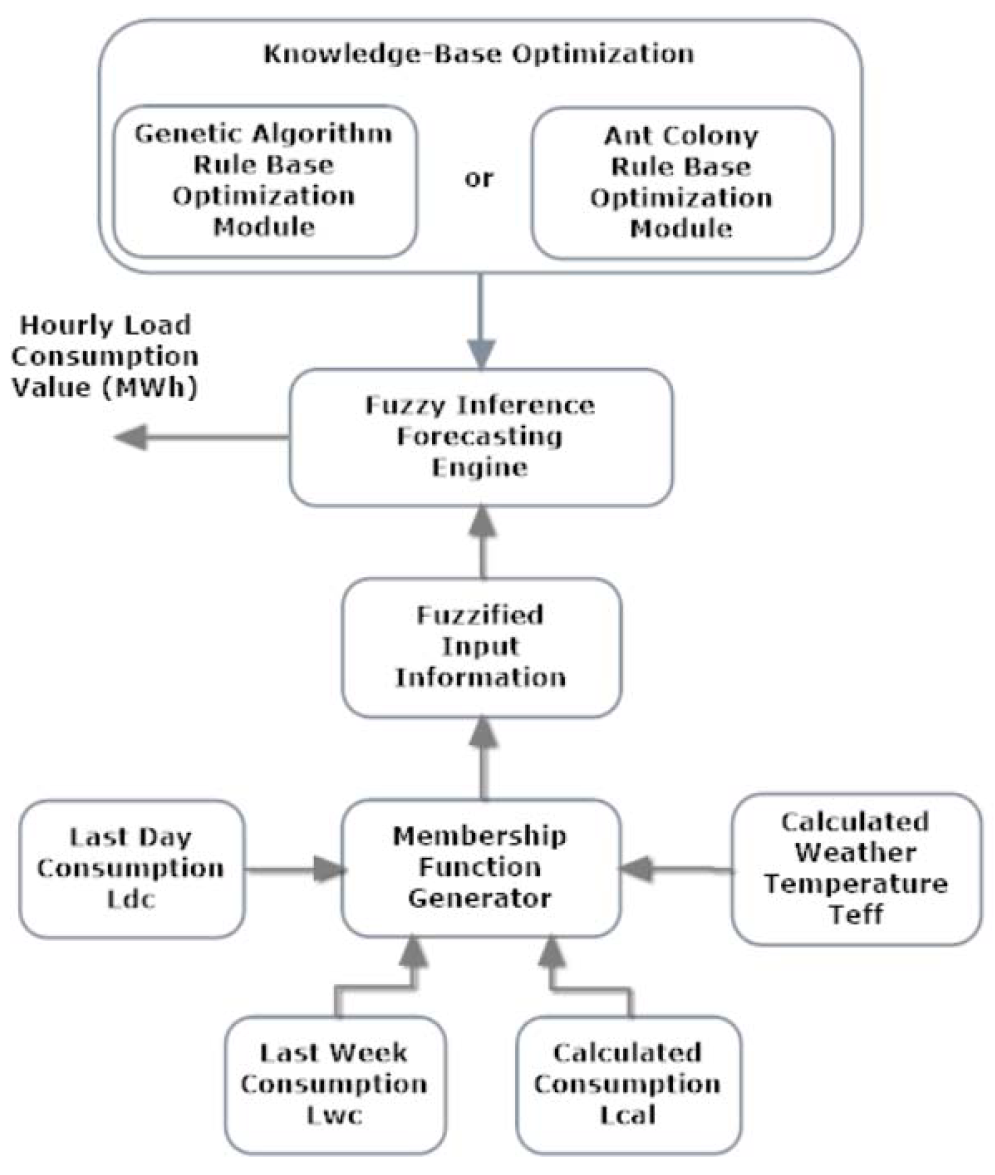
In this study, we present hybrid genetic ant colony-based fuzzy inference, which is composed of fuzzy logic and nature-inspired optimization methods. The ant colony rule-based optimization module was used for exploration (global search), and the preselected rule set was obtained. The genetic algorithm rule-based optimization module was used for exploitation (local search), and the best rule set that was found in this phase was used. The fuzzy inference module was used with both ant colony and genetic modules to get crisp hourly load consumption amounts. The general block diagram of the proposed load forecasting model is seen in
Figure 1.
The proposed models were trained and tested with historical weather temperature and hourly load consumption data obtained from National Load Dispatch Centre for the period between 2011 and 2014.
2.1. Data Set
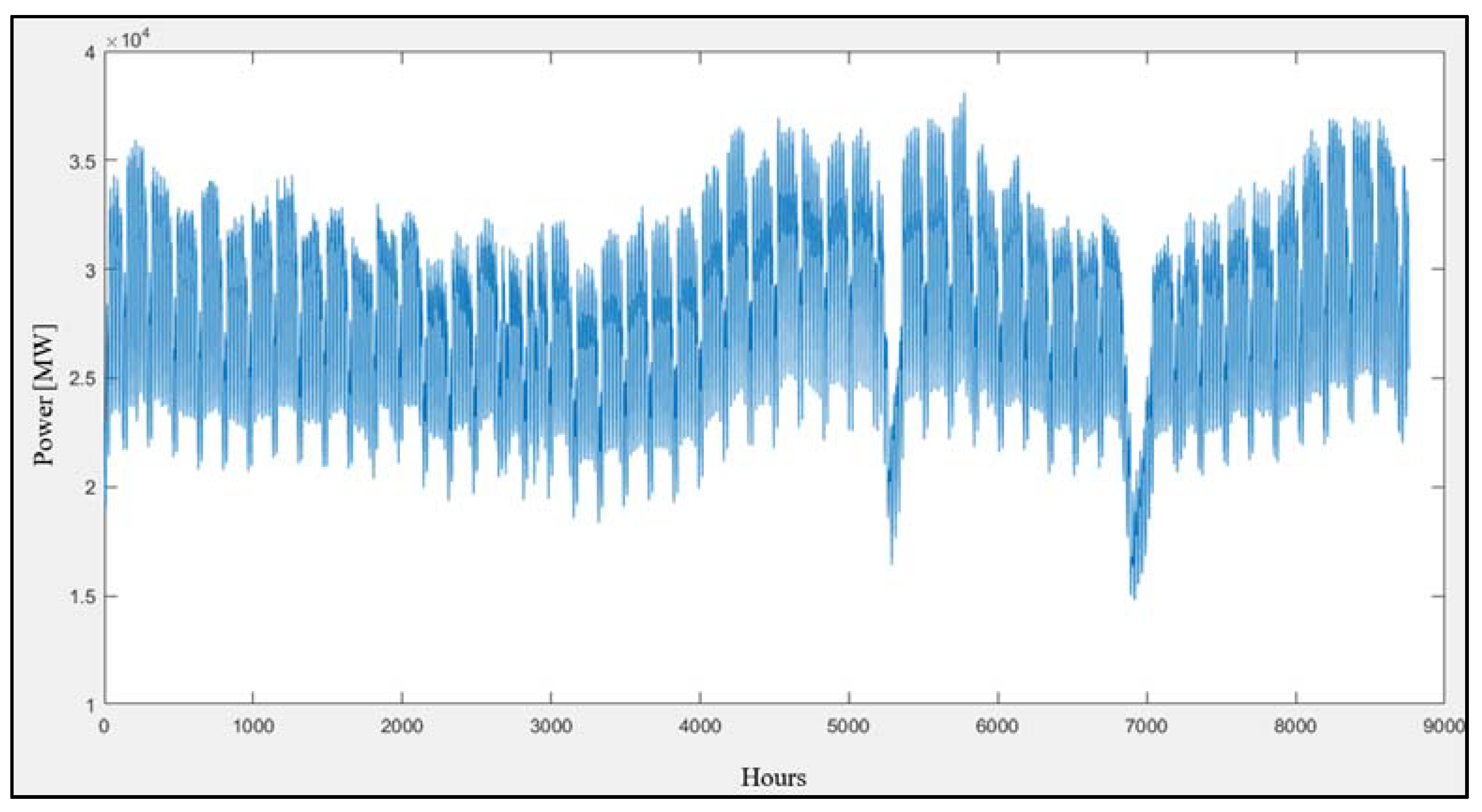
The electricity load consumption amount generally follows a routine. However, there are usually improbable changes and fluctuation. There may be countless reasons to explain these changes. Mostly, these are temperature changes, calendar effects such as formal or religious holidays, and economic and political fluctuation and crisis. The hourly-based electricity load consumption changes in 2013 are shown in
Figure 2.
In 2013, the maximum load consumption was 38,116 MWh, the minimum load consumption was 14,800 MWh, and the average load consumption was 28,003.08 MWh. The consumption values show that there is wide range of consumption characteristics in Turkey. The consumption records show that in the summer and winter seasons, consumption values are higher compared with spring and autumn. The highest consumption was recorded on 29 August as 38,116 MWh between 1 pm and 2 pm.
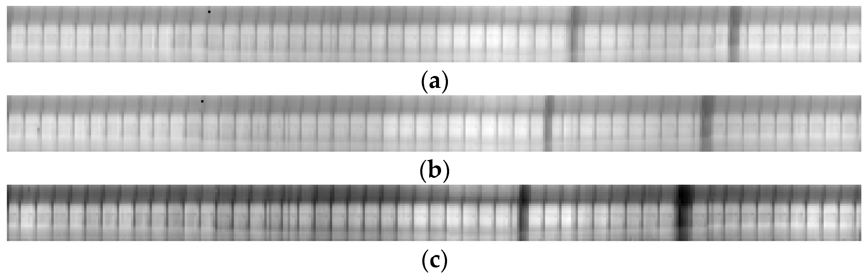
The electricity load consumption values of Turkey between 2011 and 2013 are visualized as black and white images in
Figure 3. The darker parts of the graphic are pointing out the lower consumption; nevertheless, the brighter parts are pointing out the higher consumption values. There are two areas that are darker than the others in all of the graphics; these show the religious holiday periods in Turkey. Most of the government facilities and the private sector don’t work these days; thus, electricity consumption is dramatically less than usual.
The graphics show us more valuable information about Turkey. The 2013 graphic that is shown in
Figure 3–c is generally darker than the other graphics, because there was an economic crisis in Turkey in 2013. This economic crisis started to show its effects from the end of 2012, and all of these effects are seen in
Figure 3a–c.
2.2. Last Day (Ldc)—Last Week (Lwc) Consumption
Daily electricity load consumption usually has a clear path, and studies show that there is a strong and direct relationship between load consumption and temperature changes [
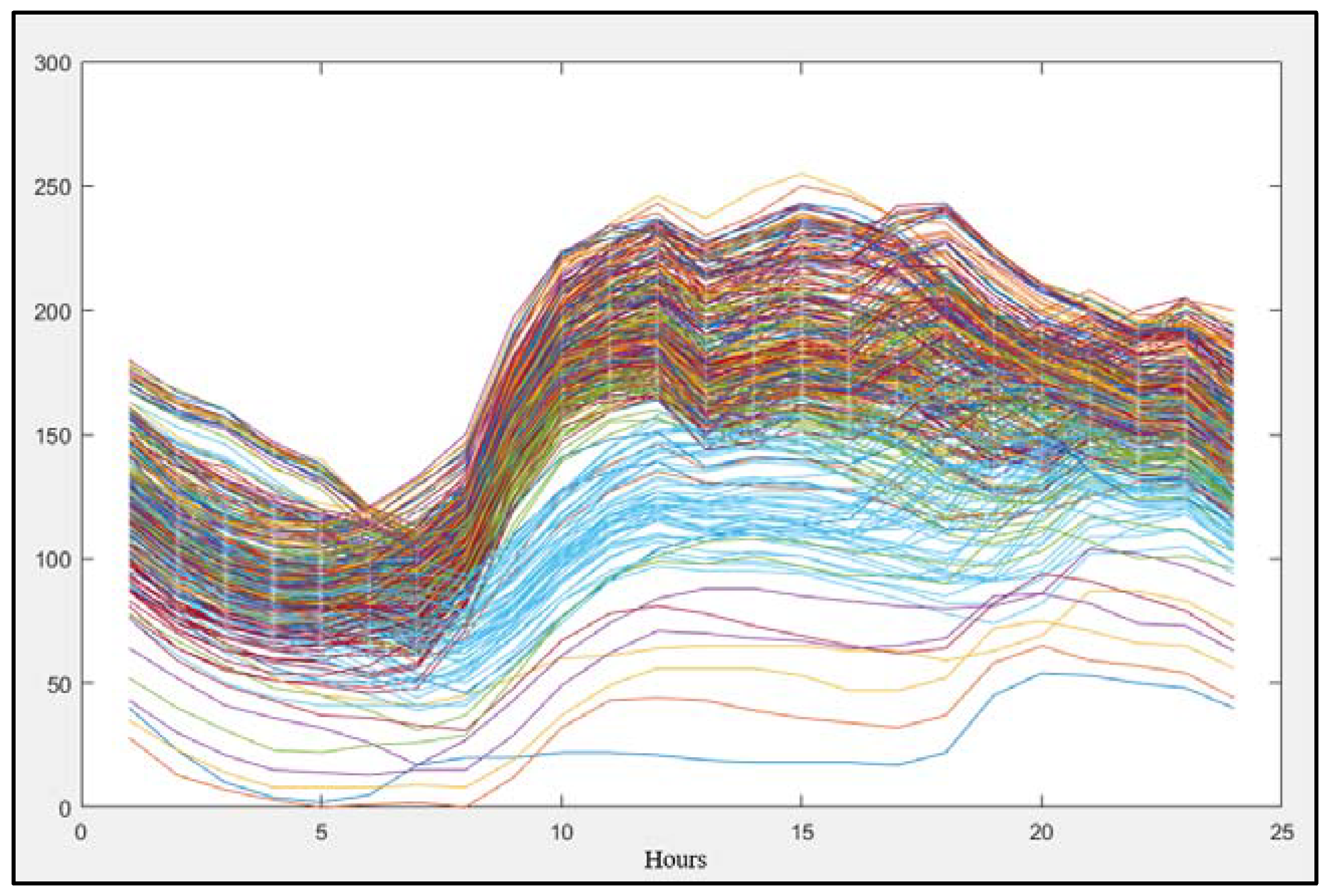
21]. The hourly-based day ahead normalized load consumption values in 2013 are seen in
Figure 4.
The daily electricity consumption pattern doesn’t change in a wide range. The load curves follow similar consumption characteristics for each day; the rises and falls are mostly similar. This consumption pattern is a useful indicator, and most of the researchers used these parameters in their studies.
2.2.1. Calculated Load Consumption (Lcal)
Daily consumption changes are remarkable indicators, but it is not enough to have a flawless load forecasting. The least squares method is the mathematical equation form that determines and visualizes the relationship in the dataset. Each data reveals the relationship between the known independent and unknown dependent variables.
The least square method was developed in the late 1700s, and is used for estimating the unknown parameters between data and the model using squared deviations [
25]. The least square method is one of the best analytical techniques for extracting valuable information from the dataset [
26]. In this paper, day-ahead weekly load changes are used as forecasting parameters. A trend analysis for the day-ahead consumption changes has been calculated using the following mathematical equations:
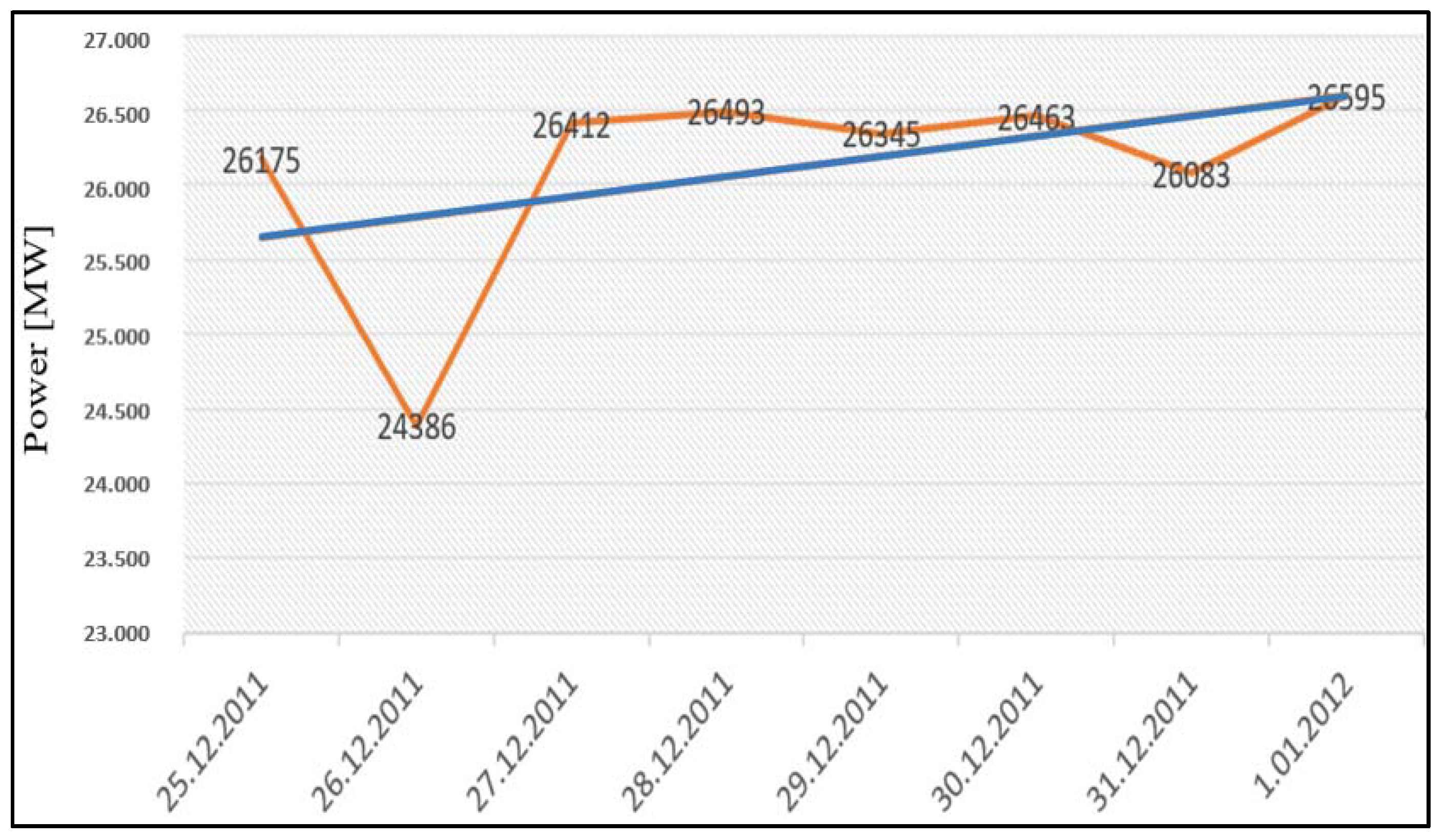
In Equation (1), L denotes the estimated hourly electricity load consumption, a denotes the load factor, b denotes the load slope, and denotes the period of load that will be estimated.
The calculated load curve (L
CAL) using the least square method is another important input parameter of the load forecasting system. Load estimation for 1 January 2012, using the data between 25 and 31 December 2011, is seen in
Table 1. Each row of the data is the measured electricity load consumption value for the same hour period (12:00 a.m. to 1:00 a.m.).
The relationship of the weekly-based hourly dataset was analyzed using the least square method, and the load trend line was determined. The target load consumption value was calculated with the equations mentioned above. The hourly load consumption data and calculated values for between 25 December 2011 and 1 January 2012 are seen in
Figure 5.
2.2.2. Temperature Data Set (Teff)
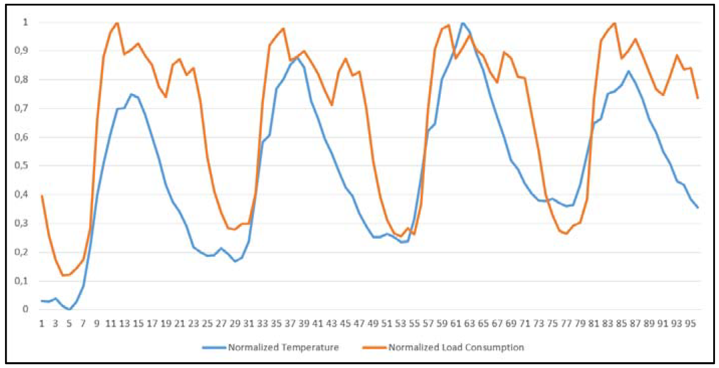
The literature research shows that there is a very strong relationship between weather condition changes and the electricity consumption amount. Temperature changes directly affect electricity consumption [
21]. The correlation between air temperature and load consumption for the period between 1 and 4 April 2013 is given in
Figure 6.
Usually, there is a linear correlation between temperature and load consumption. When temperature increases, load consumption increases synchronously. Temperature changes are crucial factors for forecasting but are not the only indicators to use.
2.3. Fuzzy Inference System
Fuzzy logic has been one of the most commonly used methods for solving engineering problems recently. Fuzzy logic methods are especially used for the planning, control, and production scheduling of power systems, and system stability management. The fuzzy logic methods and control techniques are very effective and powerful optimization tools that have many advantages, such as robustness and an ease of implementing [
27].
The fuzzy logic concept was introduced first by Zadeh in 1965 [
28]. The fuzzy approach may be briefly described as a generalized form of classical set theory. In classical set theory, every argument must be classified in an individual set or not, and any element cannot be represented by the intersection of sets. Contrary to the classical approach, in fuzzy theory, the degree of membership of an element may continuously exist. Continuous data may be expressed with membership functions [
29]. The Mamdani inference model is a well-known and used fuzzy model.
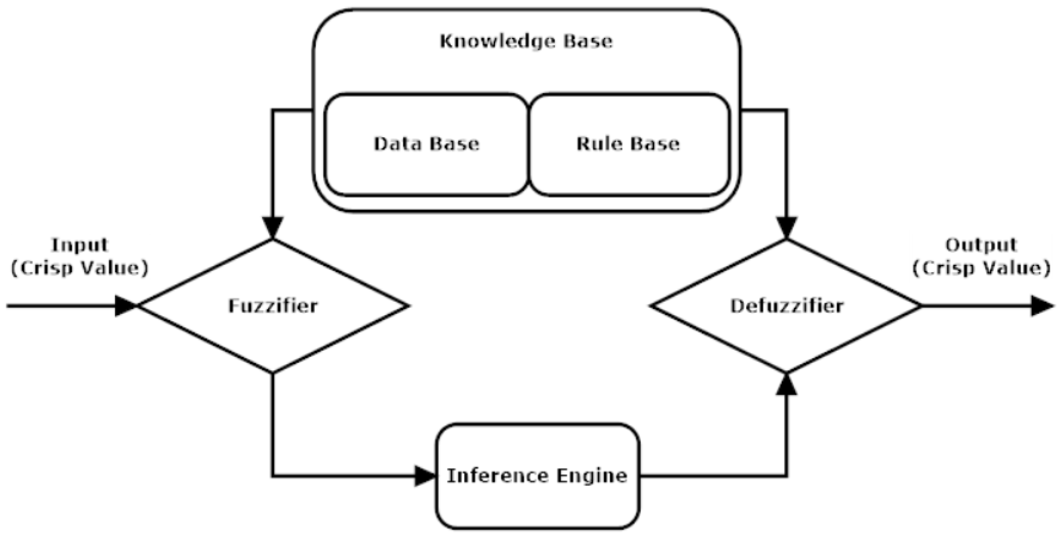
The basic fuzzy logic inference system has four main blocks, which are seen in
Figure 7. The knowledge base block involves the rule base and database, which are generally created by an expert or an optimization method. The fuzzier block is used for the transformation of crisp values into linguistic terms. Linguistic terms with membership values are processed with knowledge information in the inference module, and the results are sent to the defuzzifier (purification) module to obtain the crisp output.
In the Mamdani fuzzy approach, the defuzzification phase is evaluated with rule sentences and conditions such as those seen below:
where x and y are the first and second input variables, respectively, z is the output variable, and k is the number of rules.
There are a few important points that need to be defined very well, such as the membership function size, type, and shape. Changes to these parameters critically affect the accuracy of the system. These parameters need to be defined by an expert or through the use of optimization techniques [
30].
2.4. Genetic Algorithm
The genetic algorithm is a nature-inspired method that is based on Darwin’s evolution theory. The genetic approach became more popular through various studies and John Holland’s book “Adaptation in Natural and Artificial Systems” in the early 1970s [
31]. The literature shows that genetic algorithm methods are useful and more successful than traditional methods in solving engineering problems. Its advantages include gradient independency, a high discovery rate, and solution parallelism [
32,
33].
Genetic methods have some basic operators such as selection, crossover, mutation, and recombination. Selection operation is an elitism technique. This operation is aimed at finding the best or more useful individuals for having new and better offspring or children. There are a few selection methods used in the genetic algorithm such as roulette-wheel selection, tournament selection, and truncation selection. Crossover is a move–replace operation that is aimed at generating a new breed from existing or selected parents’ selected (single or multipoint) parts. Mutation operation is changing operation and maintains genetic diversity to the system. The mutation occurs during evolutionary operation, and works according to a predefined probability variable. Generally, a randomly generated variable for each bit in a sequence determines whether an individual bit will be changed or not. The main purpose of the mutation is to improve the genetic diversity of the breed.
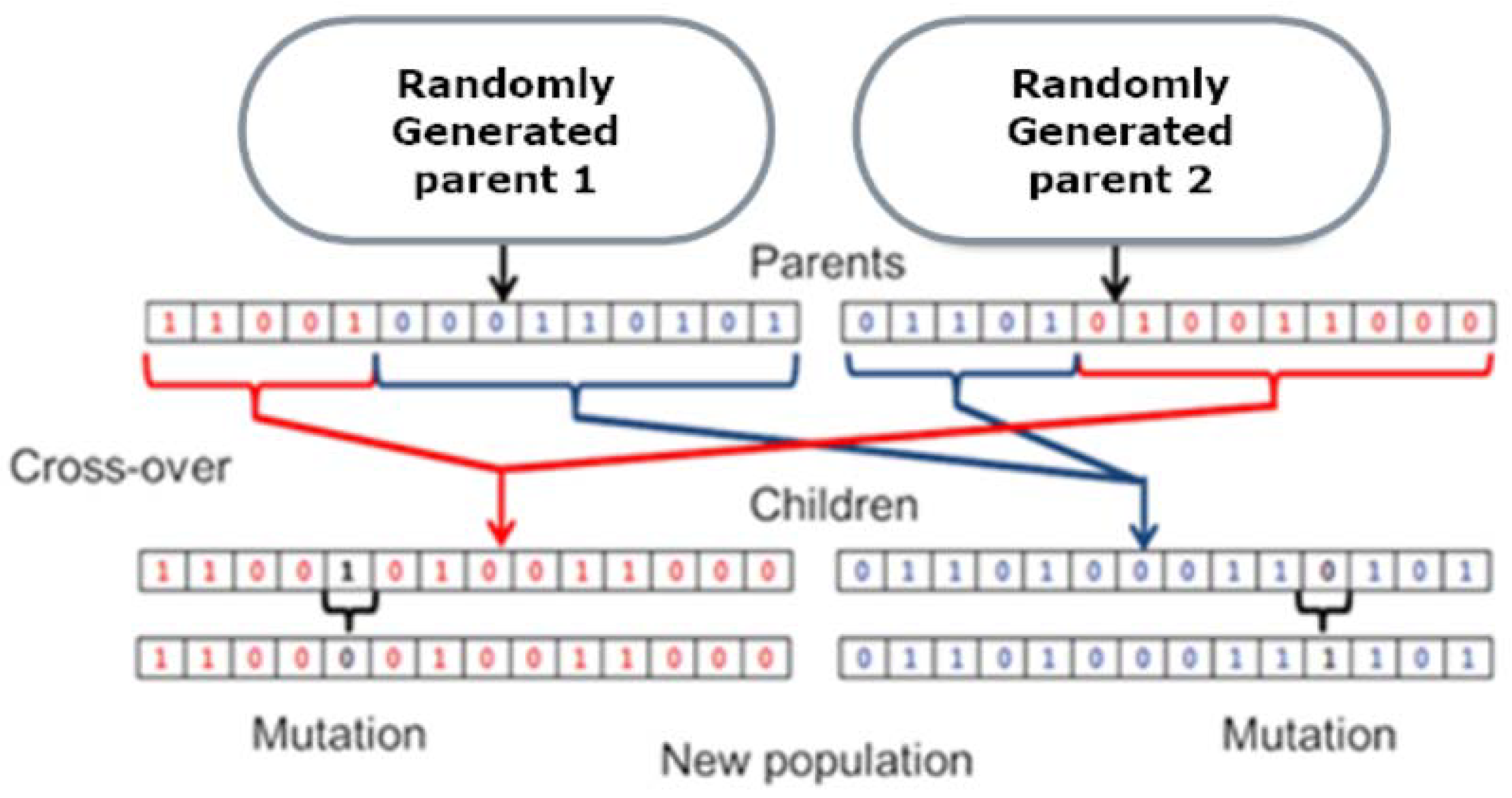
The working process of the genetic algorithm and population production process is given as a sample in
Figure 8. Two different randomly generated parents (the solution function) are seen at the top. Each parent consists of 14 binary coded gene chromosomes. The crossover point is defined before the operation, and divides the chromosome into different sized parts. These parts are used to have new children (solutions). Each child carries the parents’ unique features and characteristics. The genetic diversity of the breed is held by mutation operation. The randomly selected genes of each chromosome are changed from 1 to 0 or 0 to 1, and the generation process ends. The exploration phase is performed with the crossover operator. Sub-solutions are produced through the crossover operation, which gains a high convergence capacity to the searching system. The mutation operator provides diversity, and prevents the system from being stuck in a local optimum. The exploitation phase is performed with the mutation operation, and has a larger searching space to look for a deserved solution.
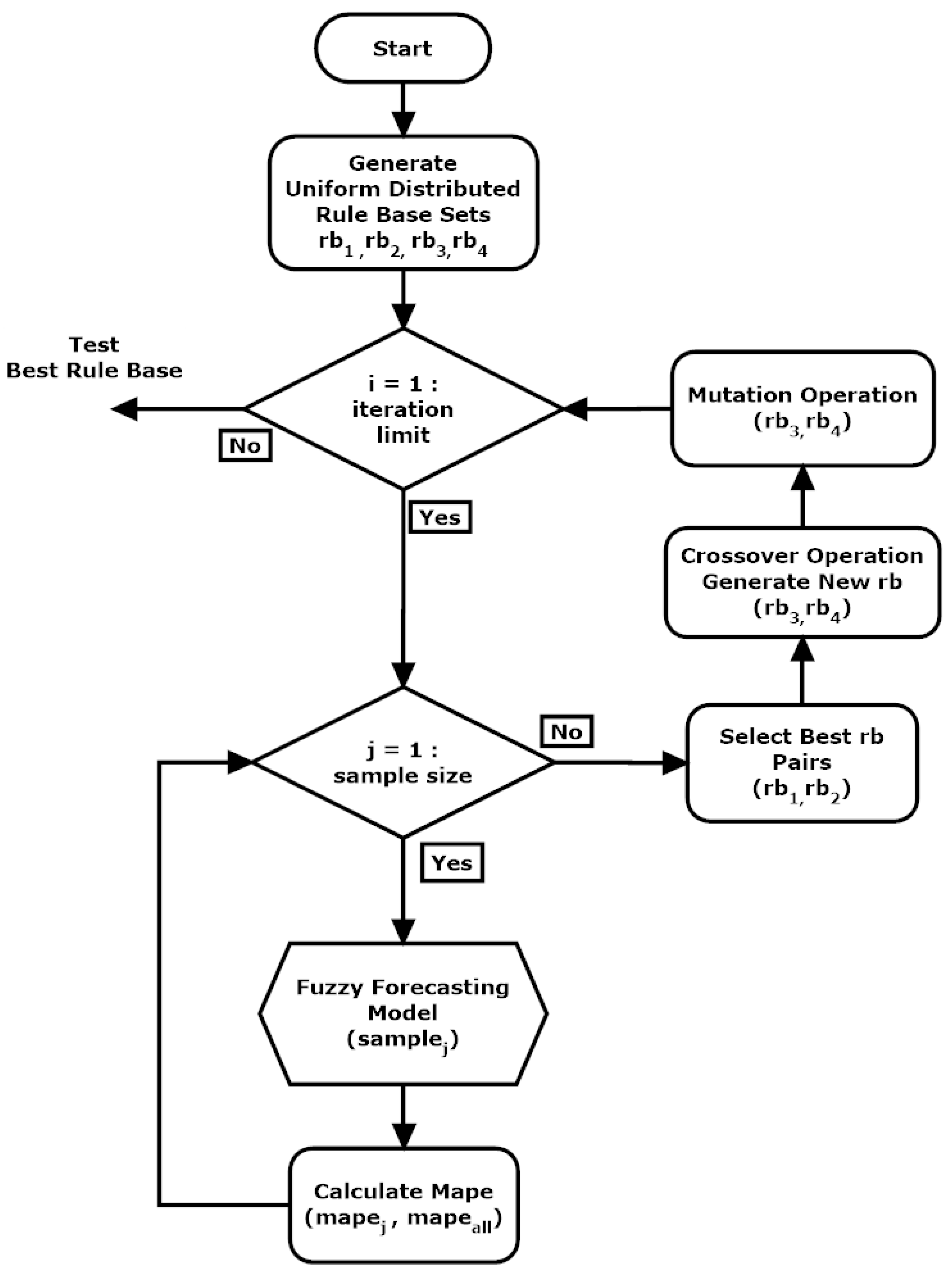
GA–FL Load Forecasting Model
The proposed load forecasting model consists of a fuzzy inference module and a genetic algorithm-based rule base optimization module. A block diagram of the proposed model is given in
Figure 9.
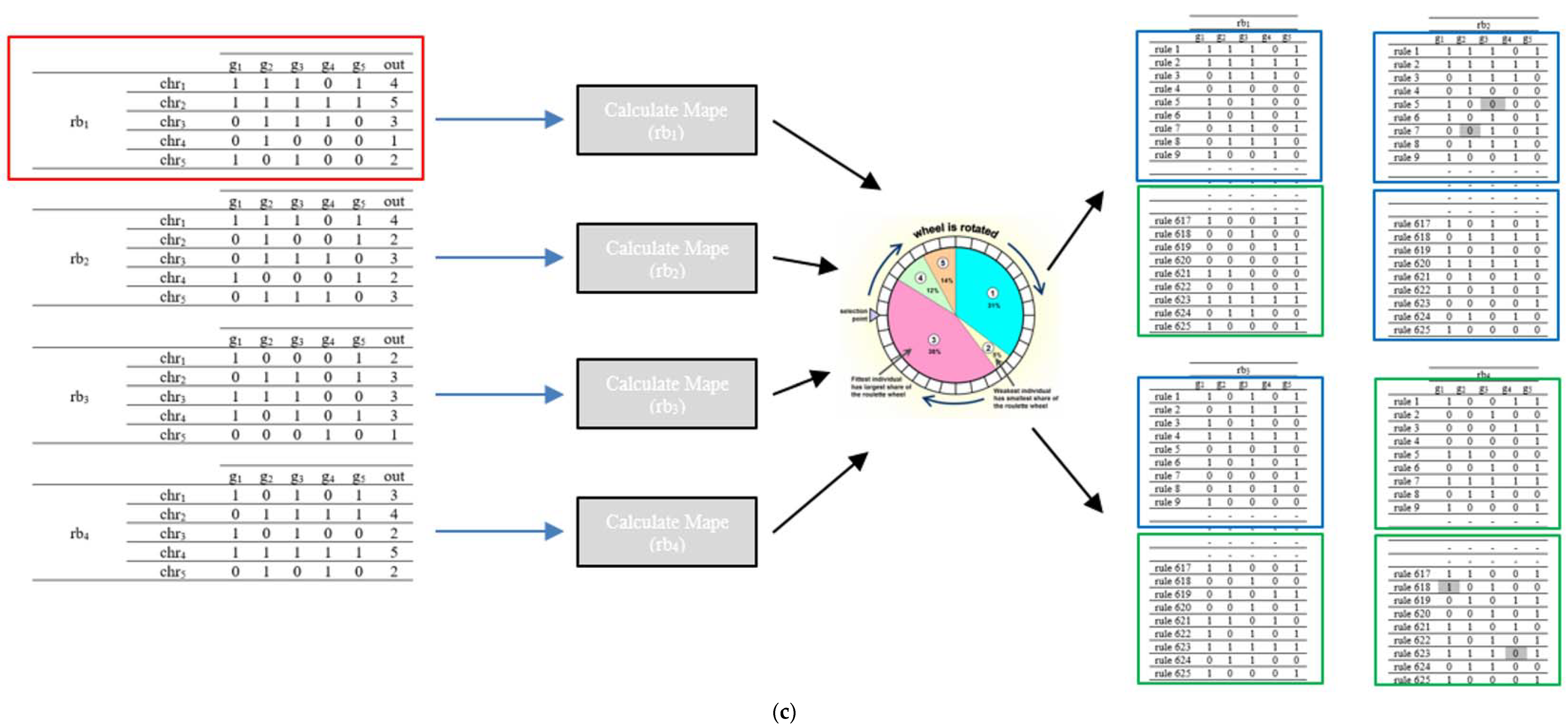
The genetic algorithm approach was applied to generate the optimal rule base set of the fuzzy load (FL) forecasting system. The rule bases were designed as five genes for all 625 chromosomes of each of four parents. Every chromosome consisted of five binary-coded genes. Uniformly distributed randomly created parent rule base sets and a genetic rule base optimization process is seen in
Figure 10.
Rule base sets were produced and uniformly distributed in the rule base generator module at the first step of the optimization algorithm. These sets were applied to the fuzzy forecasting system, respectively. The generated rule base set was used in the fuzzy inference module with a randomly selected dataset, respectively. The mean absolute percentage error (MAPE) was calculated, and the error values were saved for each rule base set, as shown in Equation (4). The calculated MAPE values were the fitness values of the rule base sets.
Actual Load
Forecasted Load
After the performance evaluation of each rule base set, the best two individuals were selected, and new candidate rule base sets were created. New rule bases were generated using crossing and mutation methods in the order of these two individuals. The evolution process continues until the iteration limit is reached.
2.5. Ant Colony Optimization
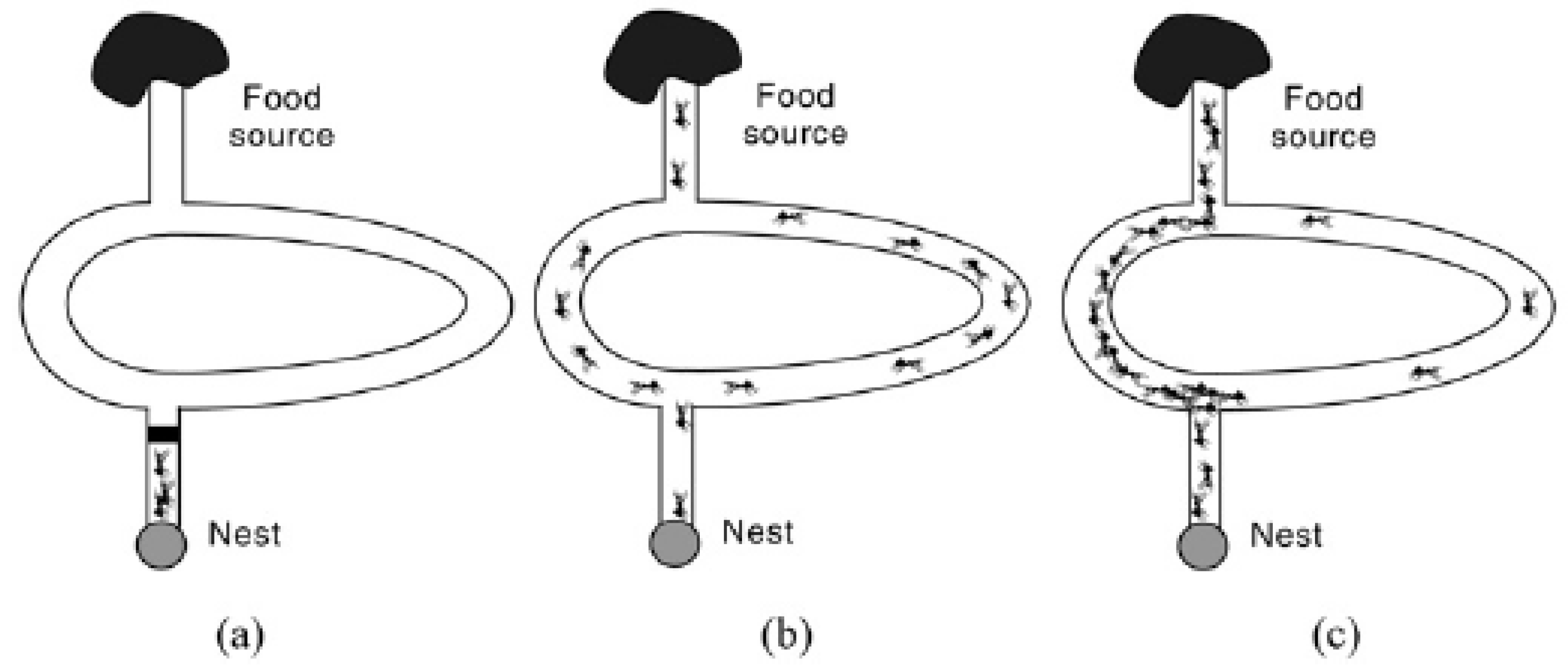
The ant colony optimization algorithm is a meta-heuristic search algorithm inspired by the strategies that ant colonies use to reach food resources [
36]. Gross and Deneubourg showed that some ant species follow a ray-type path between food resource and nest in their experimental studies [
37,
38].
At the beginning of the research, the door is closed, and ants are waiting in the nest. There are two possible routes in the system, and just one of these routes is shorter than the other one. After opening the door, the ants follow a random route to the food source, and every individual ant leaves a pheromone behind. The pheromone amount left from the pioneer ant is a clue for the ants that are following to proceed more directly to the food source. After a while, researchers noticed that most of the ants that follow take a shorter path. An experimental setup of the research is given in
Figure 11.
Dorigo et al. improved the artificial ant colony and artificial pheromone concept in their research, which was based on the experiments of Gross et al., and applied this technique to find a solution to the traveling salesman problem [
39].
Nature-inspired optimization algorithms are also used to find the best search space. There are two main basic approaches in all of the methods: global search methods (exploration), and local search (exploitation) approaches. The new solution is based on local information and an existing solution in local search methods. The hill-climbing method is a marvelous example of the local search operation. With this method, the climbing position is changed to the closest peak point at each step of the iteration. This method gains a large convergence capacity to the search system, but there is also a risk of being stuck in a local optimum. The succession rate of this method is highly related to choosing a good starting position. In the global search method, the search space is analyzed from a global perspective. The new solution is possibly found in a location far from the existing solution’s location. With this method, the convergence rate falls and the searching time gets longer, but there is no risk of being stuck in a local optimum.
The balanced implementation of the searching methods mentioned above is the most crucial factor for determining the success of the algorithm. Greater exploitation may create a faster convergence rate, but the findings may be deceptive, and might not indicate the best solution. Using more exploration stretches out the searching time and slows the convergence rate. Balancing between these techniques is also a hyper-optimization problem [
8].
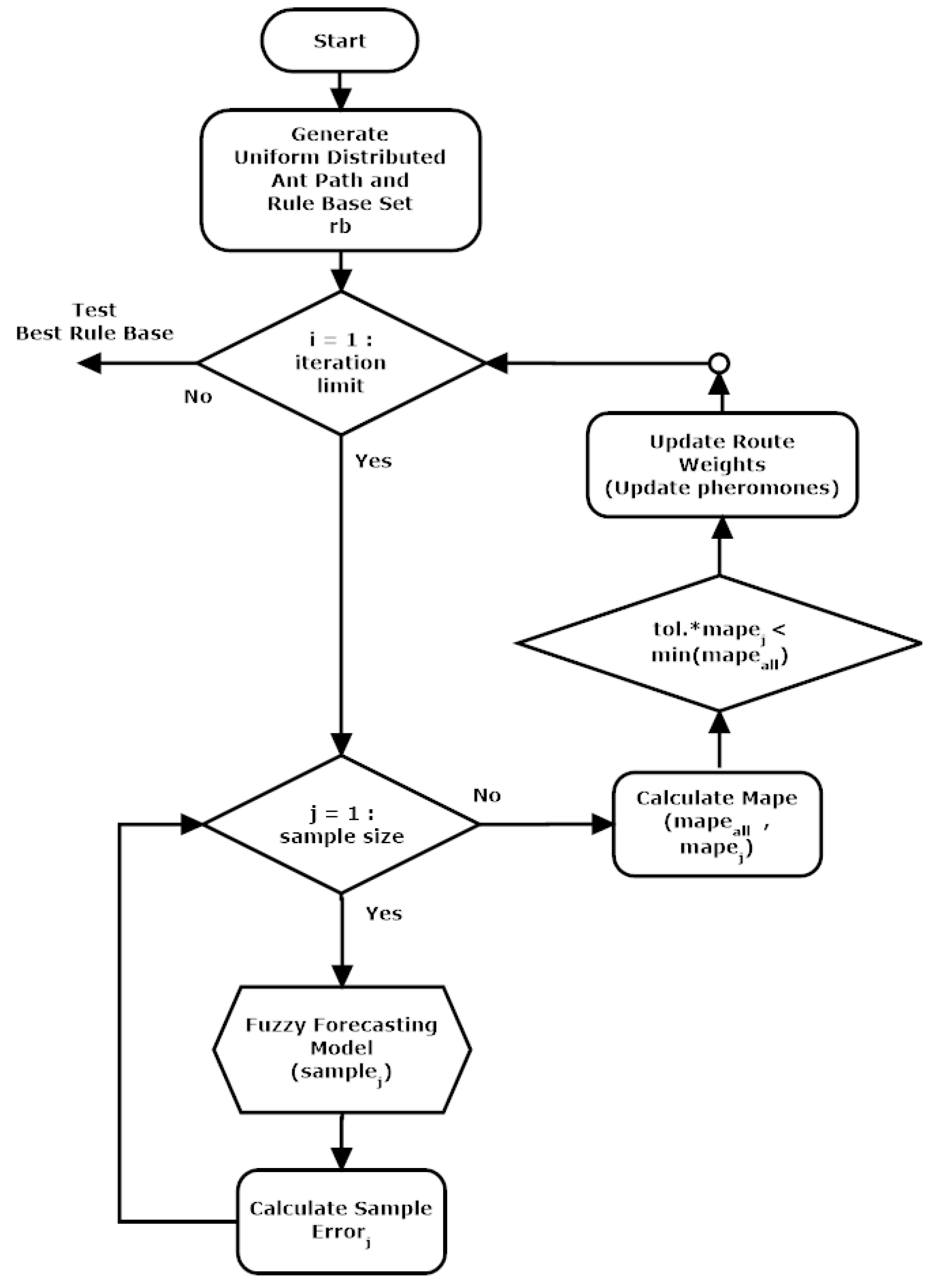
AC–FL Load Forecasting Model
The proposed load forecasting model consists of a fuzzy inference module and an ant colony-based rule base optimization module. A block diagram of the proposed model is given in
Figure 12.
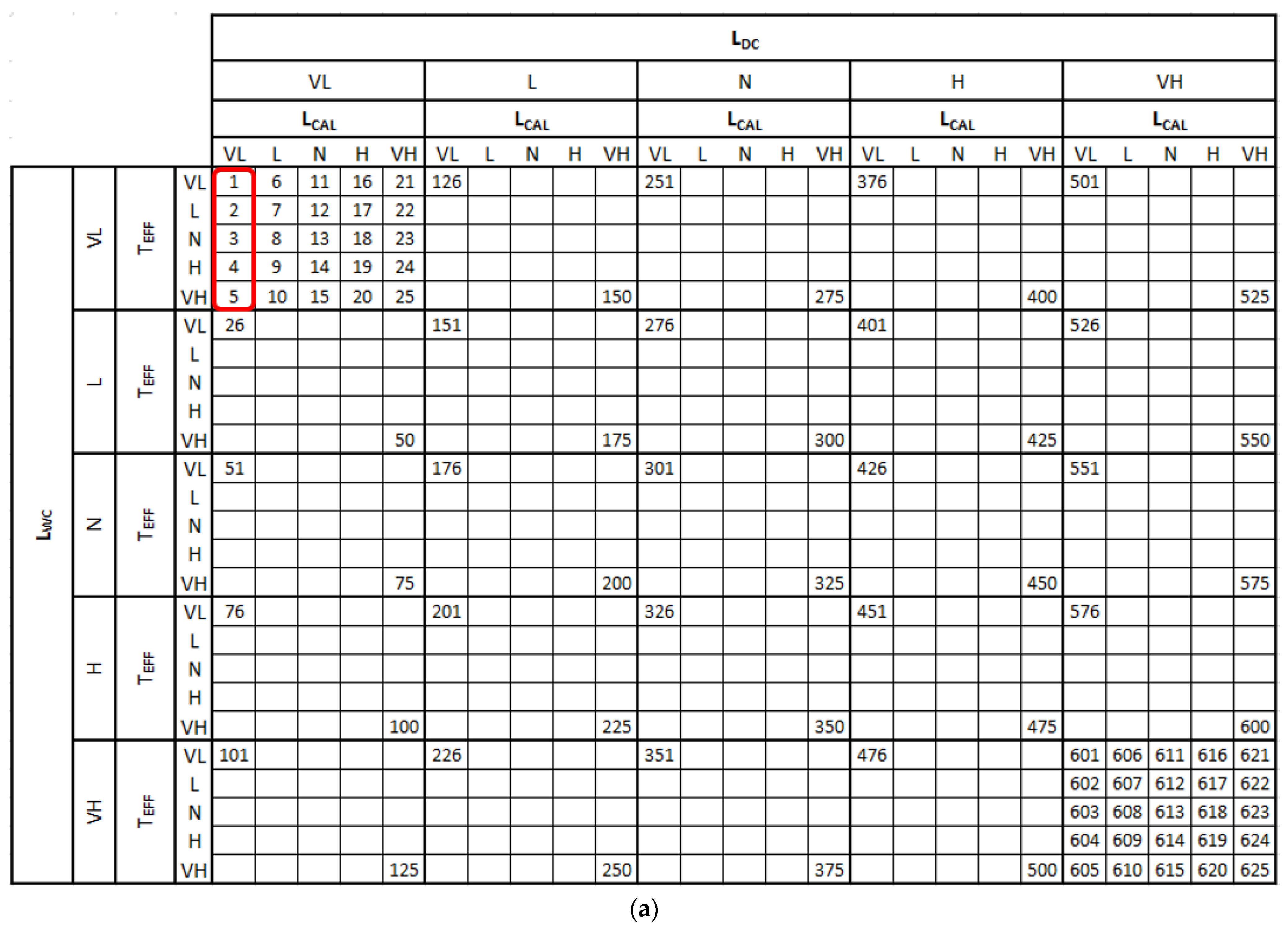
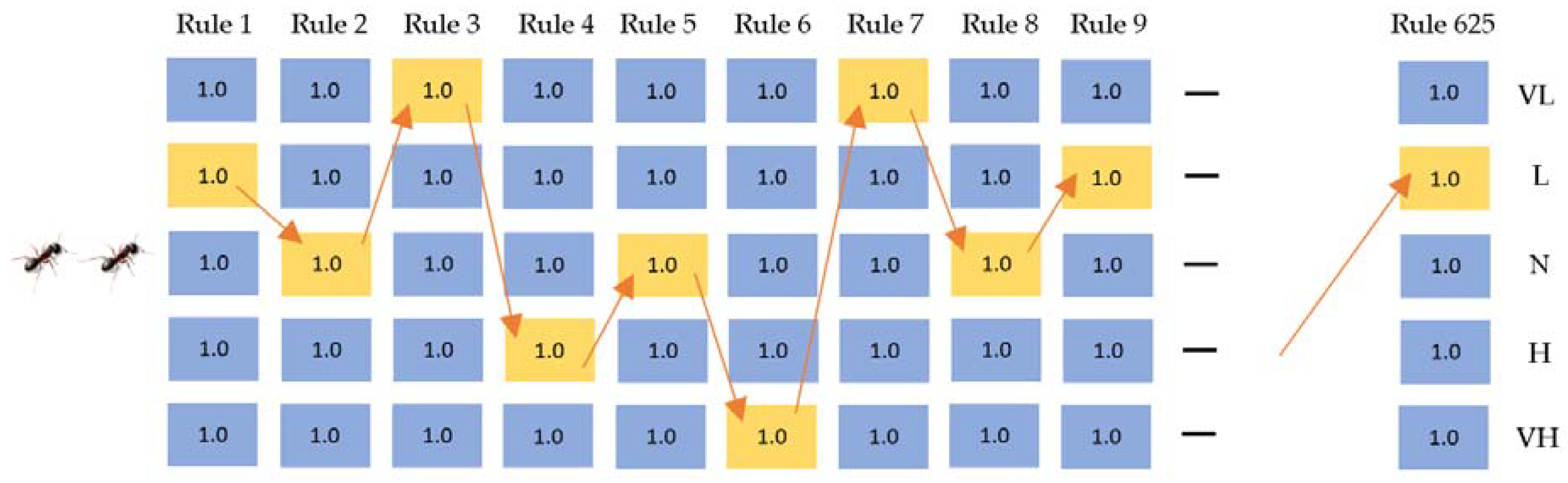
The proposed forecasting model has four input variables, and each input variable has five different membership functions. Therefore, 625 different rules covering all of the possible situations were defined in the fuzzy load forecasting model. The rule base set that was used in the fuzzy model is seen in
Table 2. These rules were then changed to the most appropriate rule base set for the system using the ant colony optimization technique. While using ant colony optimization, each rule that was used in the fuzzy inference engine is expressed as five bits of binary coded values. The binary coded rule set seems like a genetic algorithm model, but the rule set of the ant colony is unique, and only a single “1” value may be inside each rule. These positive values in each row (each rule) were used to generate a path that the ants then follow in each step of the iteration. Each column in
Table 2 denotes the linguistic fuzzified terms of the output. A sample rule base set is seen in
Table 2.
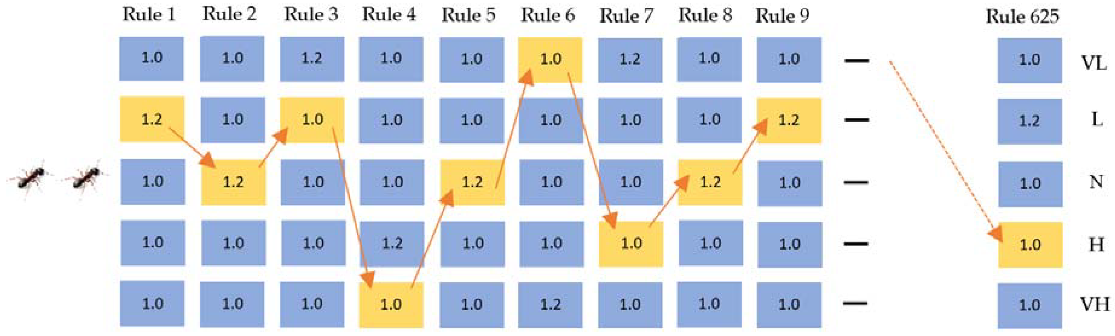
The agent operator ant follows a route that was generated and uniformly distributed in the first step of the iteration, and the selection possibility of all of the positions was defined in the same weight. A sample randomly created route at the first step of the iteration is given in
Figure 13.
After the first step of the iteration, all of the samples were evaluated with the existing rule base set, and the MAPE (obtained in the i
th iteration) was calculated. The MAPE value of the existing rule base set was compared with the predefined tolerance value, and whether existing route would be punished or rewarded was decided. If the MAPE value of the existing rule base was lower than the best-recorded value of all, then the weights of the existing path increased, and the pheromones were updated. Otherwise, the weights of existing path decreased, and the pheromones were also updated. The updated weights and the new route are given in
Figure 14.
Before the next step of the iteration started, a new route was created considering the new weights and new possibilities. Iteration continued until the iteration limit was reached or the success rate was lower than deserved.
3. Experimental Results and Discussions
In this paper, we developed two different artificial based load forecasting models. The fuzzy logic model is the main part of the system. The genetic algorithm and ant colony-based techniques were used to increase the performance of the fuzzy forecasting system.
Proposed GA–FL and AC–FL load forecasting models were trained with historical electricity load consumption and air temperature data between 2011 and 2014, as explained in
Section 2. The training and testing datasets consist of four input variables (L
dc, L
wc, L
cal, and T
eff) and one output variable (L
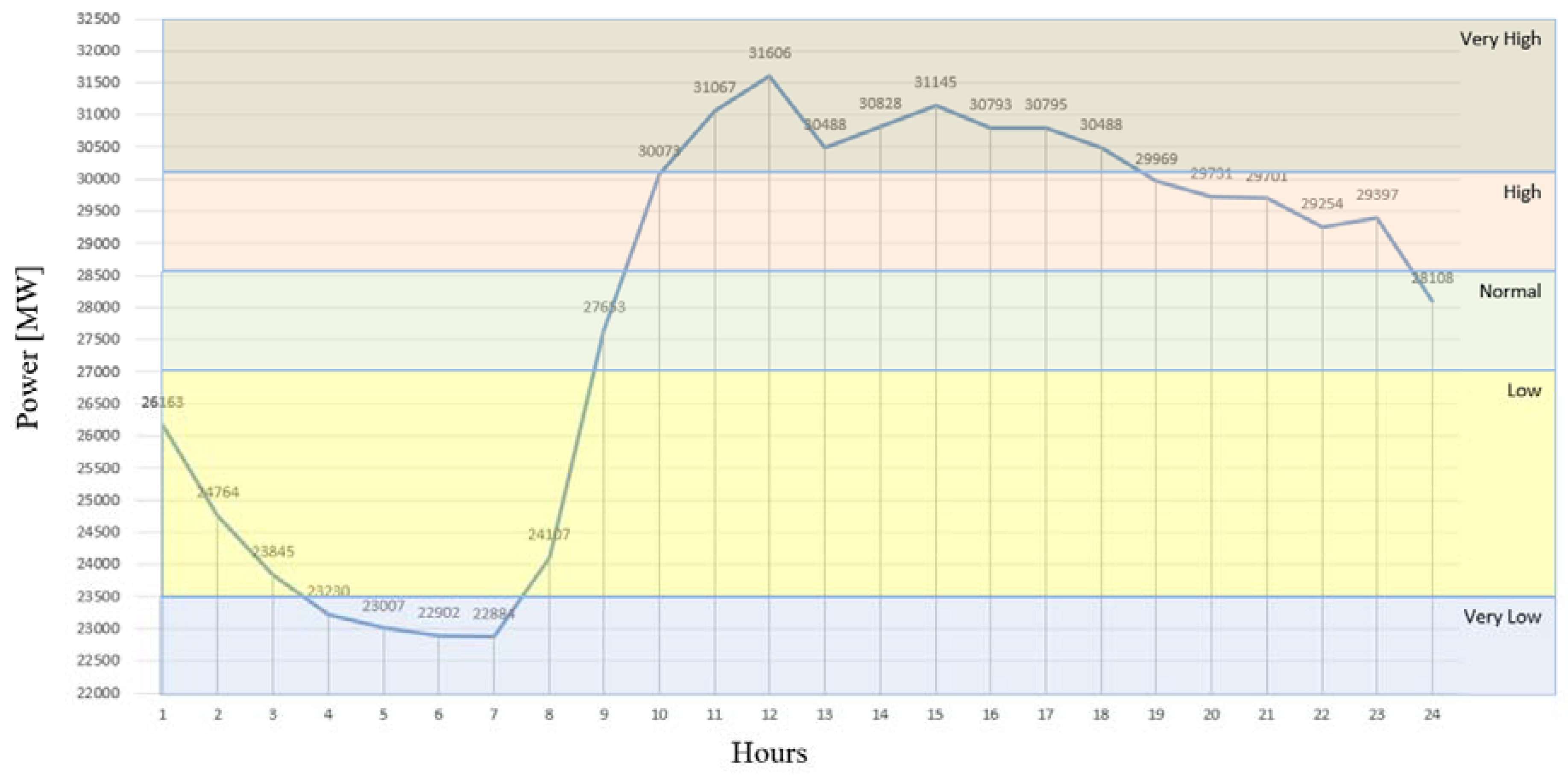
forecasted). Membership function type and values were identified by annual changes in the load consumption and weather temperature. The average load consumption values of 2013 are given in
Figure 15.
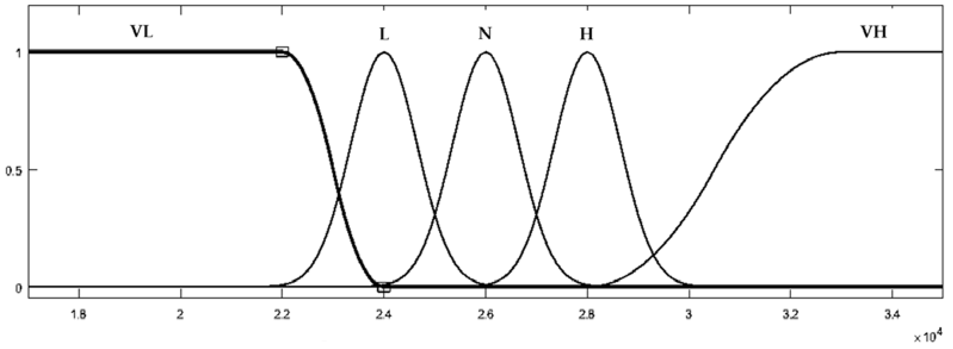
Load data was fuzzified through using five membership functions that considered the average values of 2013; the fuzzified input and output data (L
dc, L
wc, L
cal, and L
forecasted) are seen in
Figure 16.
In
Figure 16, VL denotes the lowest load value, which means very low consumption, L denotes a lower consumption than the normal level, N denotes normal consumption, H denotes a higher consumption than the normal level, and VH denotes the highest load consumption value.
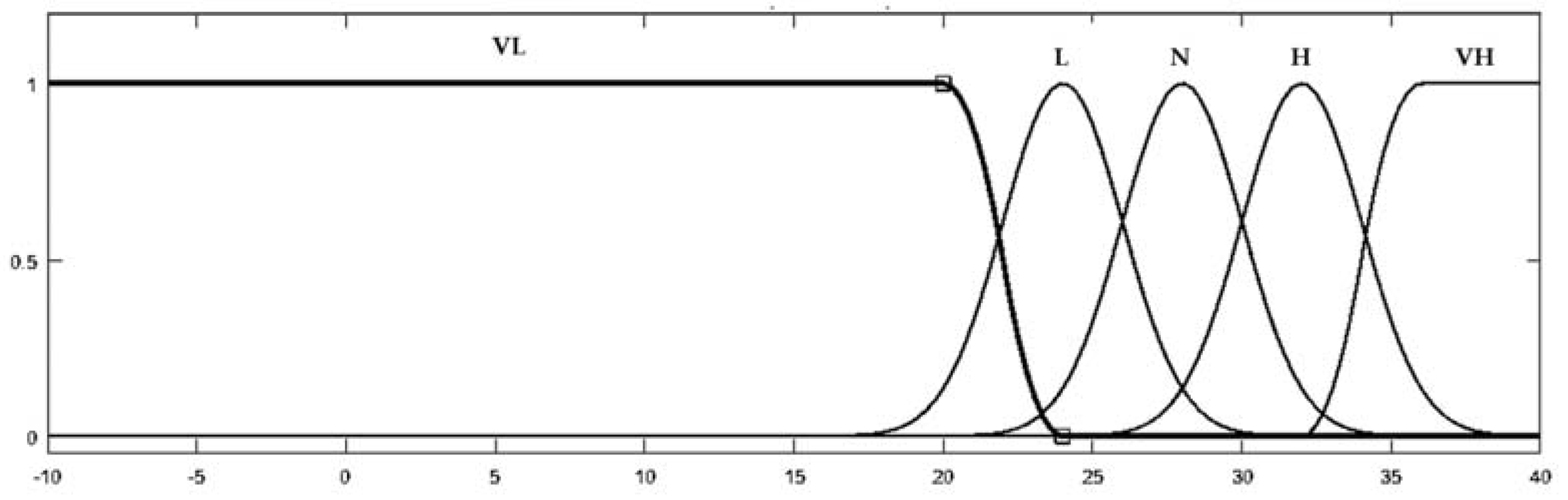
Temperature data was also fuzzified using five membership functions. Membership function values were determined considering the thermal comfort values of TS EN ISO 7730, and the fuzzified temperature data is seen in
Figure 17 [
40].
In
Figure 17, VL denotes the lowest temperature value, which means a very low temperature, L denotes a lower temperature than normal, N denotes a normal temperature, H denotes a higher temperature than normal, and VH denotes the highest temperature value.
Temperature data was provided from Turkish State Meteorological Service’s database. In this research, we observed a large scaled area in Turkey. Temperature data was collected from six different locations in Turkey. We tried to choose the best locations directly representing Turkey’s electricity consumption character. The hourly-based weather temperature data of the selected locations is given in
Table 3.
The average temperature value was calculated with hourly-based temperature data collected from six different locations. The constants (% values in
Table 3) that were used in the equation to calculate the average value were defined according to the level of economic development of the cities mentioned above, which was pointed out in the annually published report by the Ministry of Science, Industry, and Technology [
41]. After averaging the calculations, the temperature values for the last seven days were used to calculate the temperature parameters as an input variable, while also using the trend analysis methods mentioned above in
Section 2.2.1.
Both forecasting models were trained and tested with a day-ahead 24 h dataset. The input dataset consisted of the last day of consumption, the last week of consumption, and the consumption and weather temperature trends of the last seven days, which were calculated using the least square method mentioned in
Section 2. As a sample, the input dataset used for the training of both proposed models is given in
Table 4.
In summary, the input dataset consists of load consumption information and weather temperature information. Load consumption data consists of the last day of consumption, the last week of consumption for the same hour, and the consumption trend, which is calculated using the trend analysis equation mentioned in
Section 2.2.1.
Weather temperature information is obtained in a two-stage process. First, the weighted average air temperature is calculated using temperature data collected from six various locations in Turkey. Then, the air temperature trend is calculated using the trend analysis equation mentioned in
Section 2.2.1. Lastly, the whole forecasting and optimization process uses the 24-h dataset.
3.1. GA–FL Simulation Results
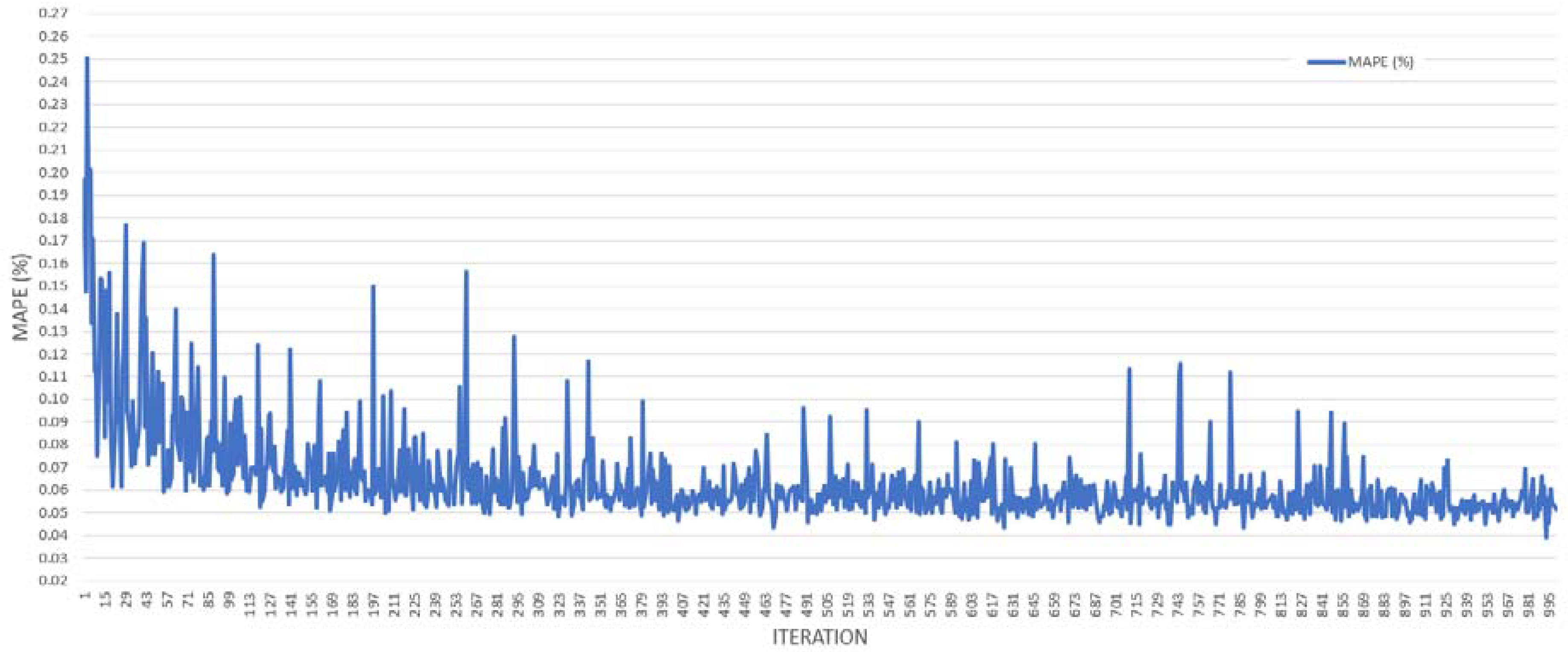
The proposed GA–FL model was trained with a randomly chosen training set and tested data for a specific period, such as a monthly or weekly dataset. The results showed that the GA–FL model gives satisfying results for the specific part of the testing data, but couldn’t have full coverage. In other words, the final rule base set that was created with the optimization model didn’t fit for properly testing the entire dataset.
In order to reach the best rule base set, four different rule base sets consisting of 625 random rules were defined as a binary system to the optimization system in the initial phase. The performance value of each rule base was measured separately for the same training set for each step of the iteration. The results of this measurement are shown in
Table 5.
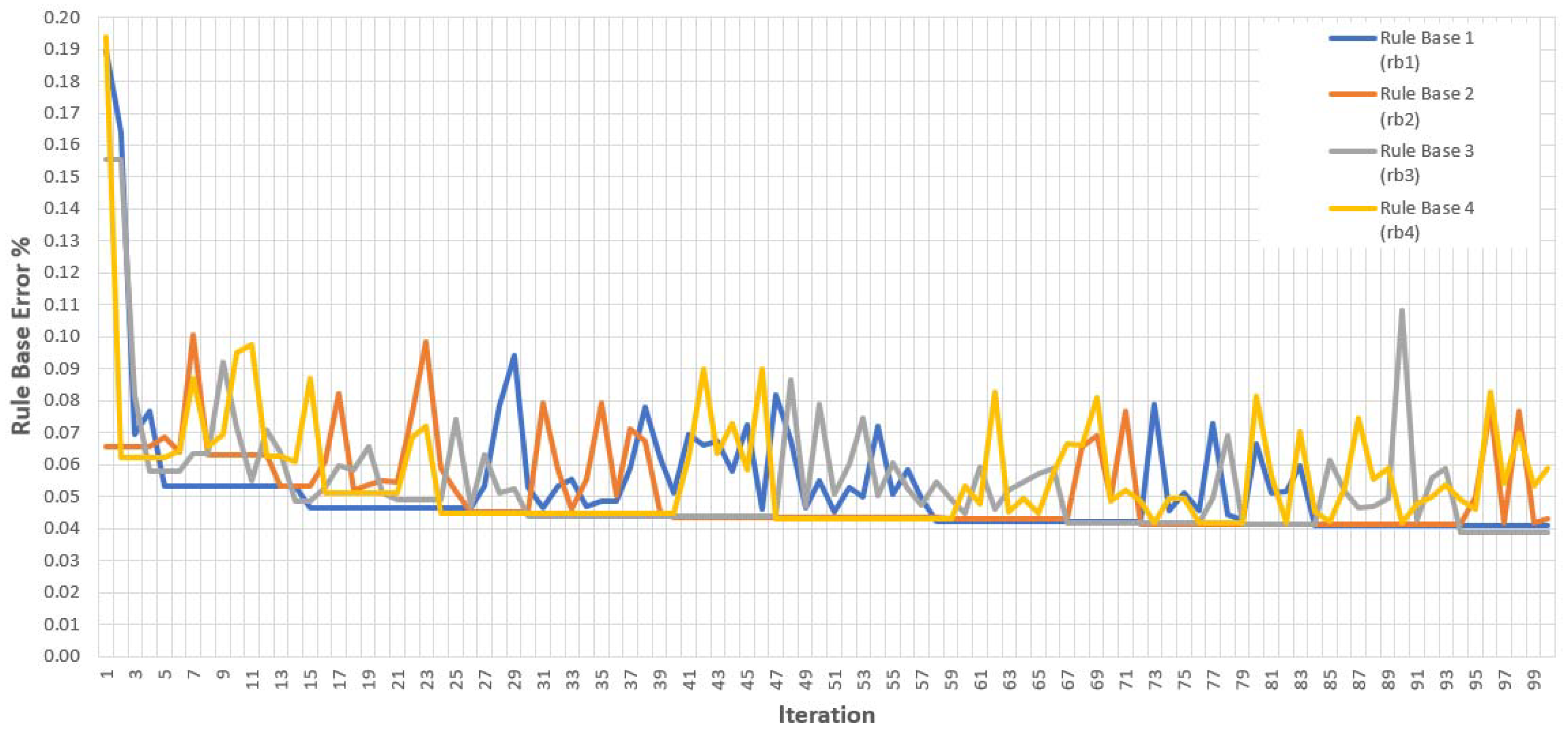
After each step of the iteration, selection, crossover and mutation operations that were designed in compliance with genetic algorithm methods were used, and a new rule base population was produced. The performance values of each rule base set and the optimization process are given in
Figure 18.
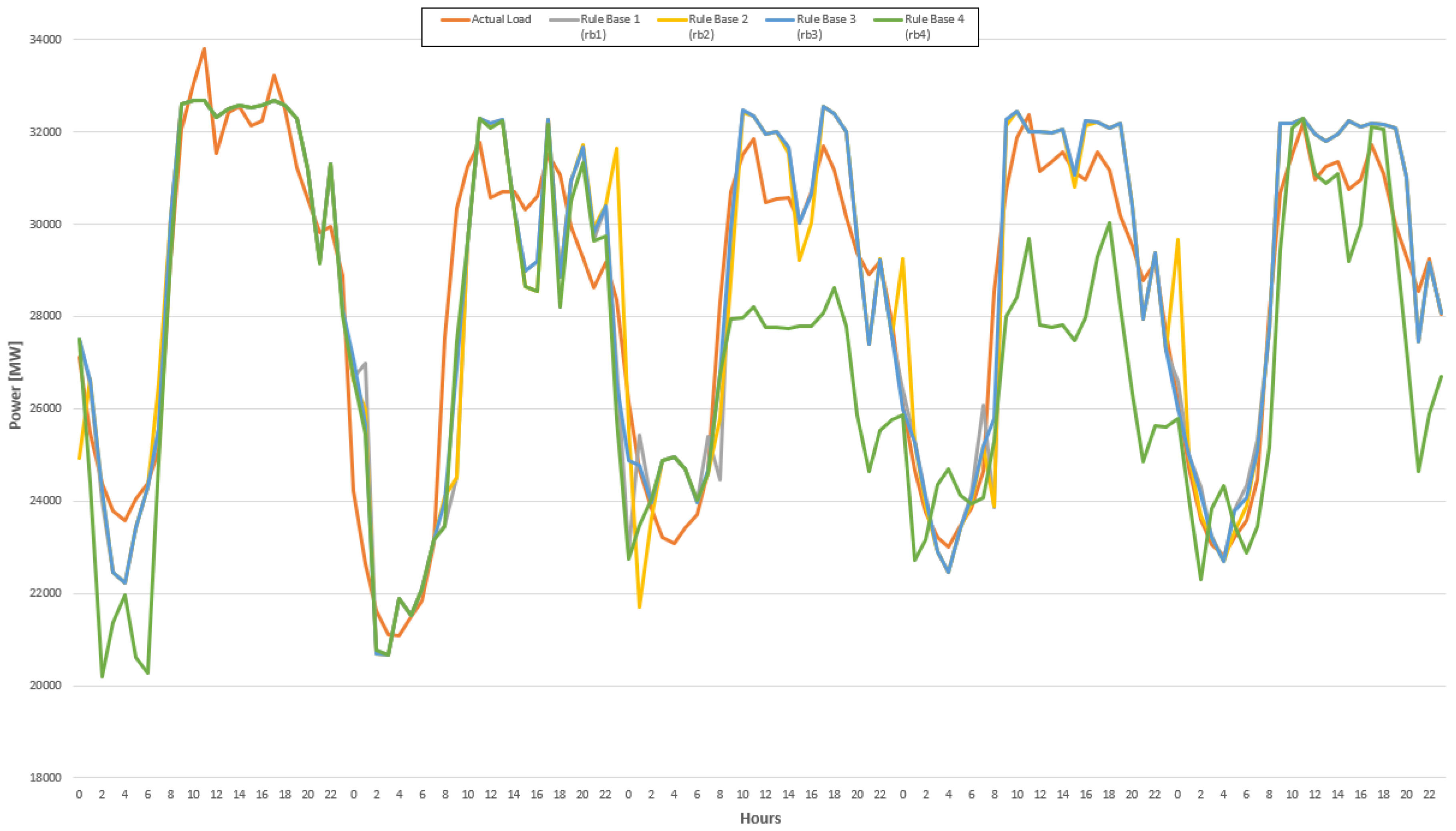
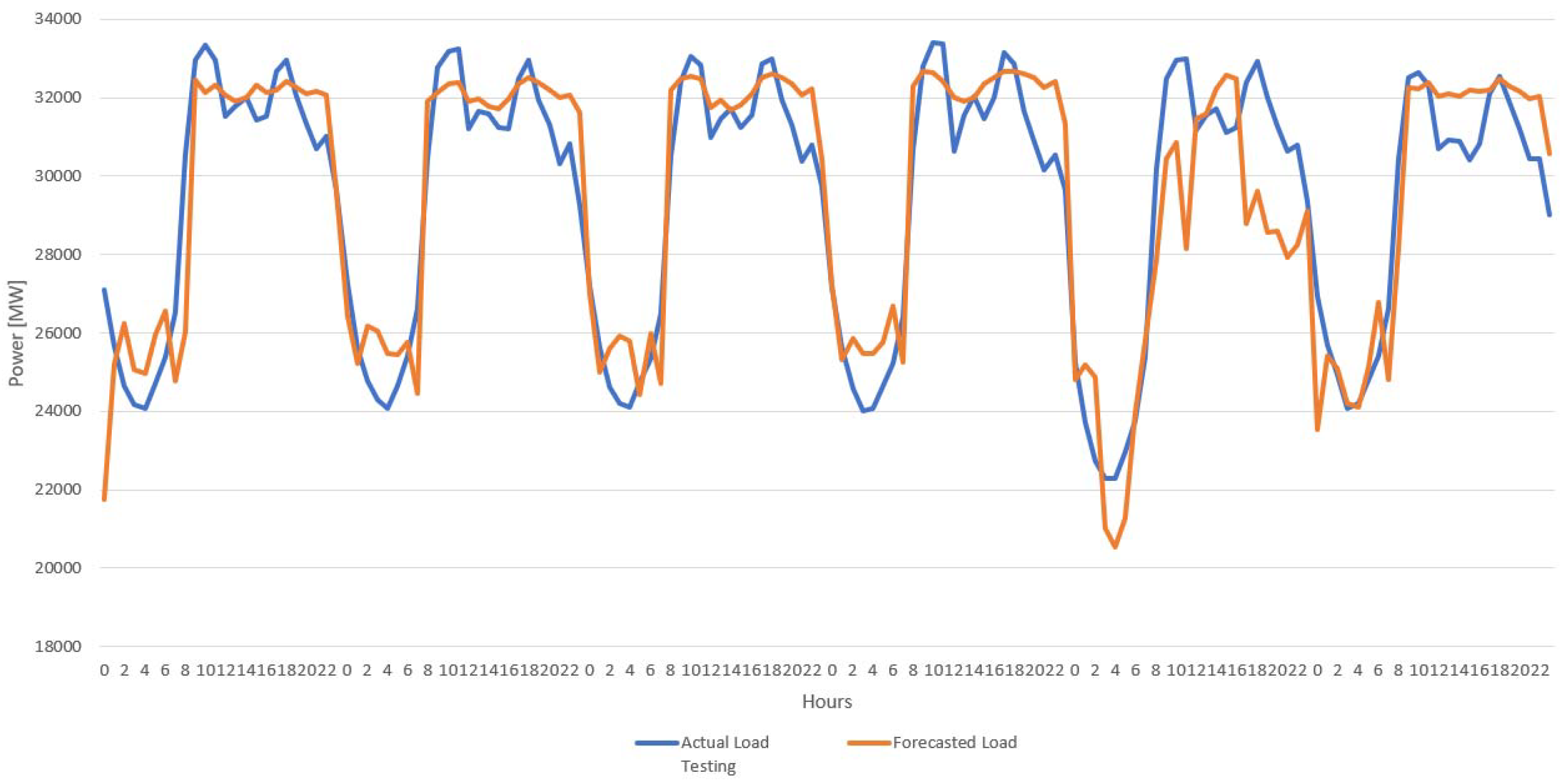
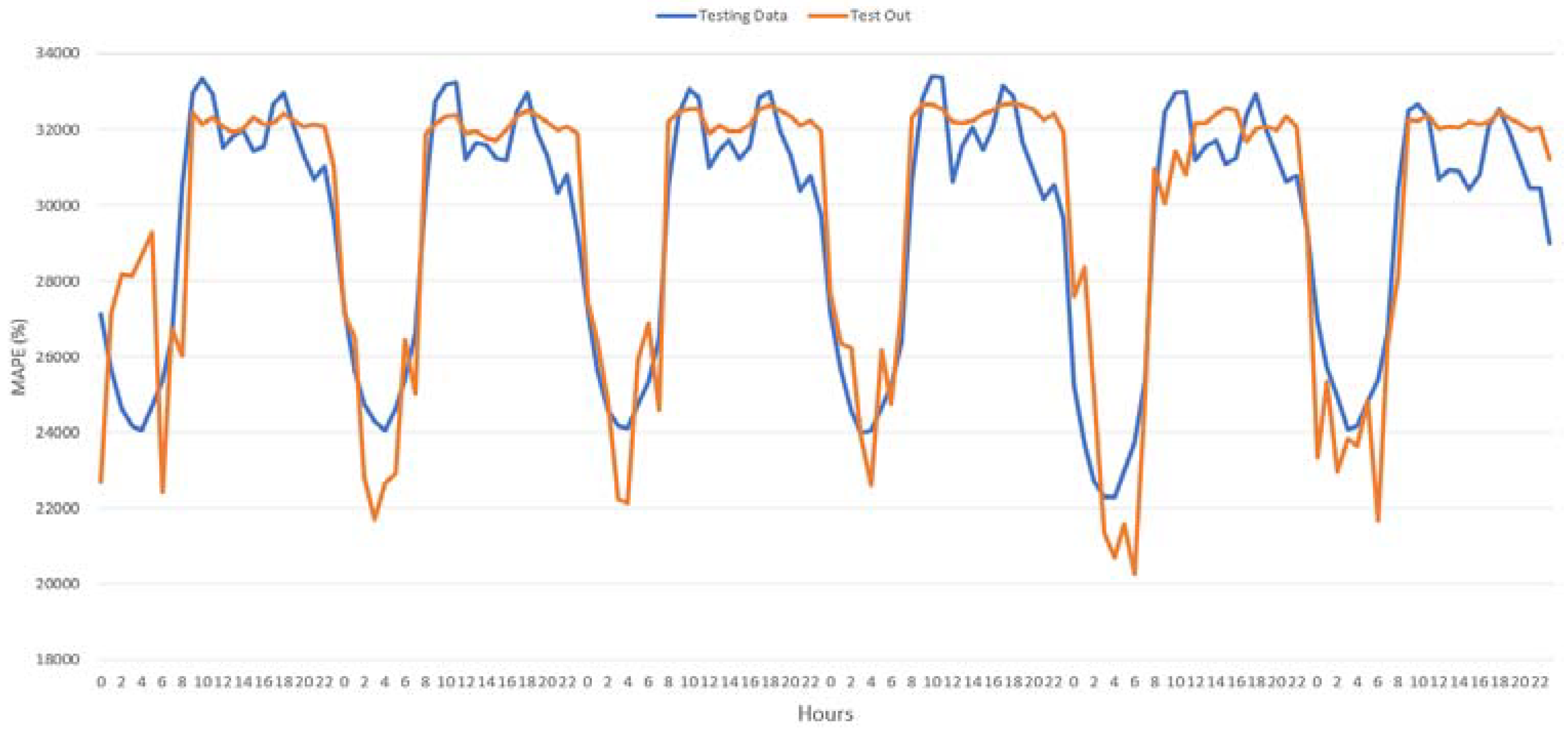
The proposed GA–FL load forecasting model was trained with a monthly weekday dataset between 2011 and 2013, and tested with a monthly weekday dataset of 2014. Each rule base that was obtained at the last iteration of the optimization process was tested with the training dataset, and some of the forecasting results of the proposed forecasting model for the training and testing processes are shown in
Figure 19 and
Figure 20.
The proposed GA–FL model consisted of four individuals, and the mutation constant was 1%. The script was executed for more than 20 different runs with 100 iterations in order to have statistically meaningful results.
Each genetic rule base set after the optimization process was tested and compared with the actual data in
Figure 19 for the same consumption period. The optimal rule base set was then tested with actual data, and the results are seen in
Figure 20.
3.2. AC–FL Simulation Results
The proposed AC–FL model was trained with the data from 2012, and tested with the data from 2013 for the same monthly period. The simulation results showed a downward trend for the MAPE value of the optimization system since the first step. The system learned with both negative and positive information. When the MAPE value was worse, it showed that the existing choices on the ant path route were not proper for the fuzzy model, that this route was punished by giving fewer weight values, and that it consequently decreased the selection possibility of the path in the next step. When the MAPE value was better, it showed that the existing choices on the ant path route were more proper for the fuzzy model; thus, this route was rewarded with higher weight values, and it increased the selection possibility of the path in the next step.
After a while, in the late phase of the iteration process, as shown in
Figure 21, differences in the MAPE values decreased dramatically. This situation showed that the route was optimized, the agent ants almost followed the same path, and similar rule sets were applied to the system in each step of the iteration process. The route optimization process and MAPE values of the ant rule base sets are seen in
Figure 21.
The proposed AC–FL model was trained with 1000 virtual agent ants. In each step of the iteration, when an agent ant followed a route, which meant a new knowledge base of the fuzzy model, the weight matrix was updated. This route was also constantly updated with other pheromone amounts, which were calculated using the tolerance value that was defined at the beginning of the iteration process in the script. The pheromone constant in each iteration was calculated according to the performance of the virtual agent ant.
The training and testing values of the proposed AC–FL model are given in
Figure 22 and
Figure 23. The proposed model was trained with the monthly-based dataset for the same weekday periods in 2013 and 2014.
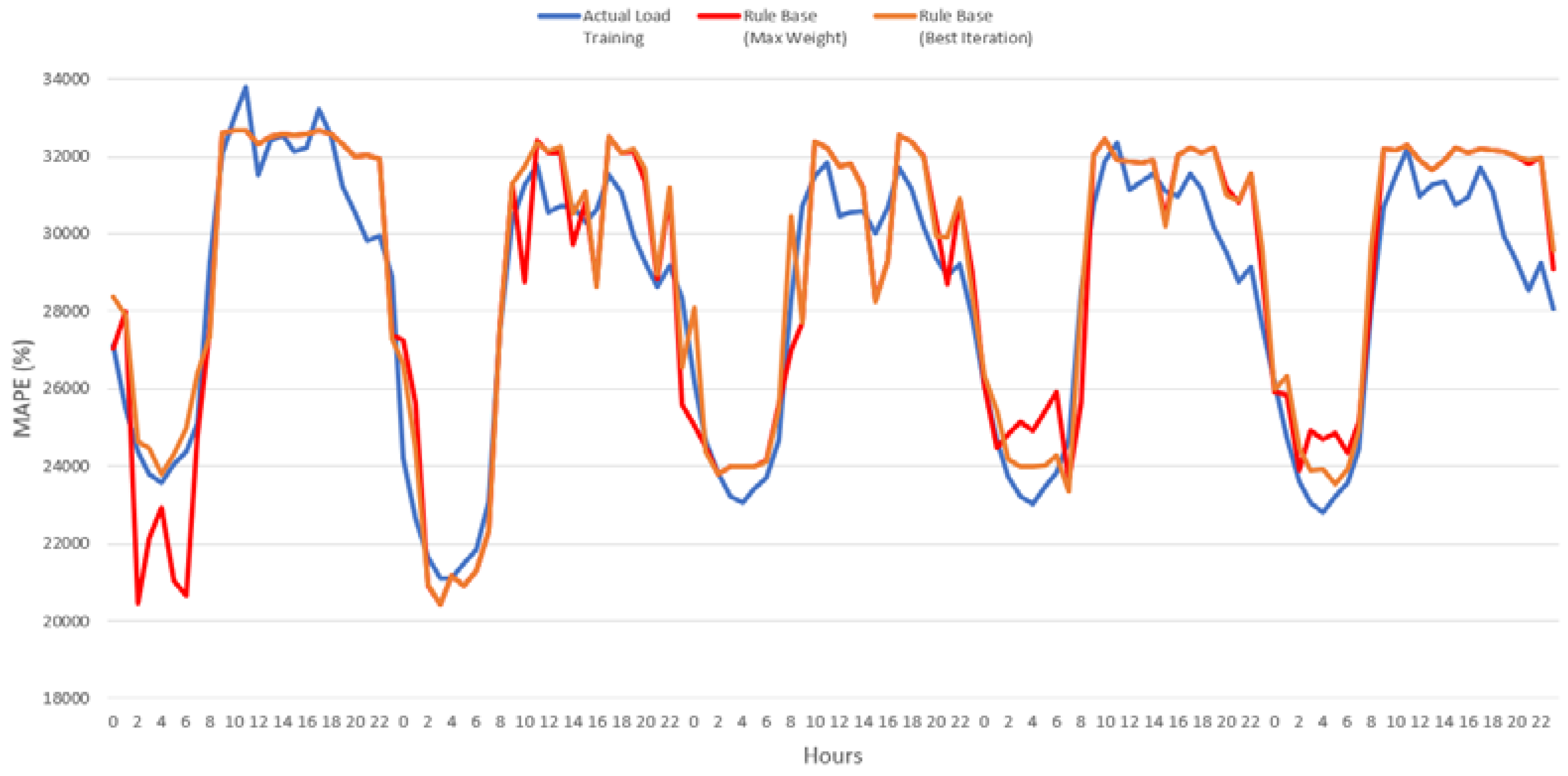
The ant colony optimization process is aimed at finding the best rule base set that will be used for testing with the target data. At the end of the optimization process, two different rule base sets were improved at the same time. One of these rule base sets gave the best training error value, which was saved and labeled as the best iteration. The other rule base set was obtained indirectly by measuring the maximum weights of each rule of the rule set’s weight table. A comparison of these rule sets is given in
Figure 22. Comparative information on the rule sets helps choose the rule set that will be used for testing.
The compared results of the proposed models for the same testing dataset are given in
Table 6. Both models were trained and tested with the same monthly dataset. The training dataset included weekdays in February 2013, and the testing dataset included weekdays in February 2014.
The main reason for presenting the results from weekday periods in this paper is that weekday load consumption characteristics are more challenging than weekends. Therefore, the weekday results of the proposed models were presented. Also, the month of February is a kind of transition period of the year; it contains the features of four seasons, and thus was chosen as the case scenario period.
3.3. Comparative Results
The performance of the proposed forecasting models is compared with the multiple linear regression (MLR) model. The multiple linear regression (MLR) method is a well-known statistical based estimation method that is commonly used as a benchmark model for comparing forecasting models. Multiple linear regression analysis is a kind of simple linear regression analysis. MLR is used to define the correlation between two or more independent variables and a single continuous dependent variable. MLR is also used to identify whether a confounding influence exists. It ensures a way of adjusting for potentially confounding variables that have been included in the model.
Both the MLR and proposed forecasting models are trained and tested with same dataset. The statistical parameters and results of the proposed MLR model are given in
Table 7 and
Table 8.
MLR model has four independent variables: the last day of consumption (L
DC), the last week of consumption (L
WC), the weekly load trend (L
CAL), and the weekly air temperature trend (T
EFF). The proposed linear model is given in Equation 5. The proposed MLR model was trained with a training dataset, and after analysis, the coefficients of weights (w
0 to w
4) were determined. The analysis results and coefficients that were used in forecasting hourly-based consumption are summarized in
Table 9.
The linear forecasting model (LM) is:
A performance evaluation of each forecasting model has been conducted using the same dataset for training and testing. MAPE values have been calculated and used to determine the monthly forecasting performance of each model. Each model was trained using data obtained during the same period. Trained forecasting models were tested using data obtained during the same period. Training and testing phases were performed using the same monthly data sets for different years. The obtained results of the proposed models for the same period, 29–30 January 2013, are presented in
Table 10 and
Table 11.
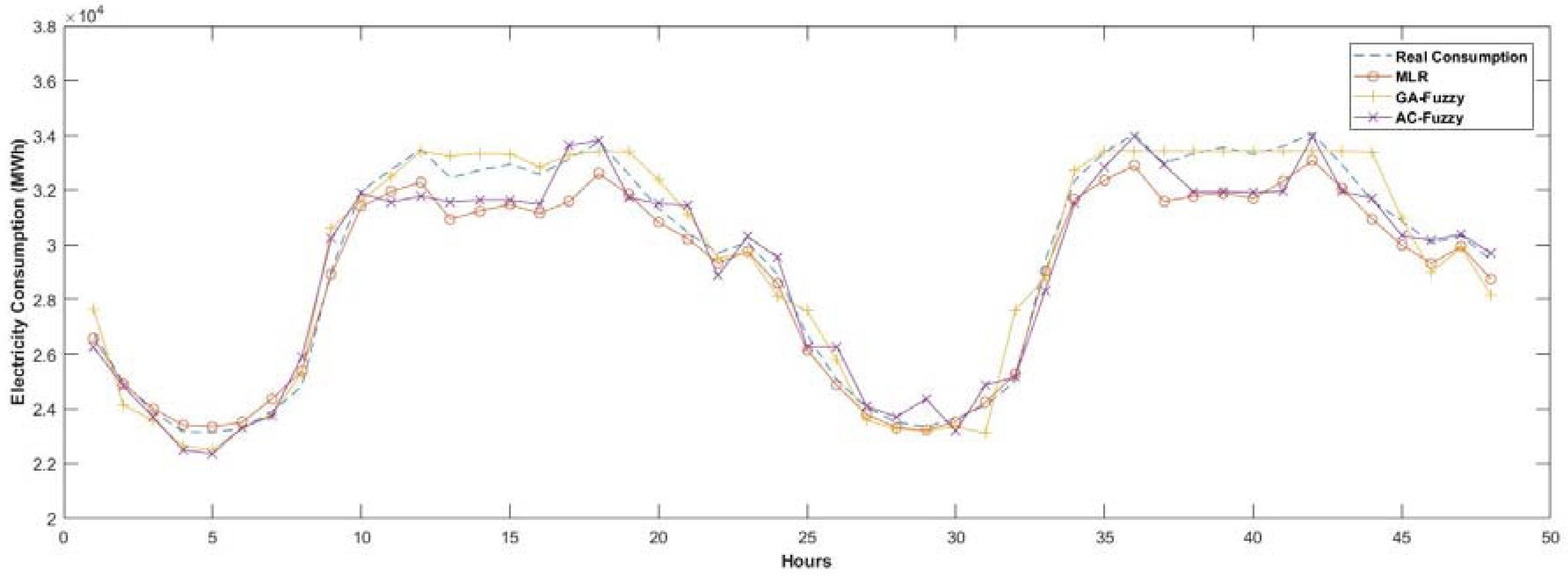
Firstly, as seen in
Table 10 and
Table 11, the proposed mature-inspired technique-based forecasting model has smaller MAPE values compared with the statistical-based model MLR model. As seen in
Figure 24, artificial intelligence-based models have better adaptation and yield more promising results than the statistical-based model in a nonlinear consumption zone. As with many statistical models, the MLR model provides more successful results, as expected in the linear zone.
4. Conclusions
Short-term electricity load forecasting has become one of the most popular research topic in recent years, and many inspiring types of research are seen in literature. Load forecasting has a leading role in the planning and management of power plants and production facilities. Research studies in the literature show that the load consumption pattern is highly related to air exogenous factors such as the weather condition, consumption time, day type (working, holiday etc.), seasonal effects, and economic or political changes. Therefore, several types of solution methods are required; here, these methods have also been improved in order to get better estimations.
In the literature, there are many studies on load forecasting that use fuzzy logic and artificial intelligence optimization algorithms and methods. Here, these fuzzy models have been improved with expert insight and adaptations. Therefore, the ability and knowledge depth of the experts has directly affected the succession rate of the system. When the input variable and membership function sizes get larger, the knowledge base, rule base size, and number of rules also enlarge. So, the fuzzy model needs to be optimized, whether classical or artificial intelligence methods are used.
In this paper, hybrid genetic–fuzzy and ant colony–fuzzy short-term load forecasting models were proposed. Artificial intelligence (AI)-based optimization methods were used to deal with the struggles in rule base definition that were mentioned above. The result show that intelligent optimization methods give promising results in load forecasting. The succession rate of the proposed system was measured by using MAPE, and the results showing that the proposed method has a 3.389% forecasting rate.
As a result, we developed fuzzy logic-based load forecasting models for estimating hourly-based electricity consumption. The literature research and observations showed that the definition of the knowledge base is a major factor in having a successful forecasting rate. Moreover, when the size of input variables and/or membership functions size grows, the knowledge base becomes dramatically more complex. We developed GA–FL and AC–FL hybrid models using nature-inspired optimization methods to deal with knowledge complexity. The obtained results showed that the proposed models are more successful than the standard fuzzy logic approach that is typically seen in the literature, and proved that Nature-Inspired (NI) based methods help when working in a more flexible estimation environment.
As a limitation of the proposed methods, in some cases, such as while working with a low-temperature period of time, some of the rules that are highly related to high-temperature periods may not be active in the optimization process. These inactive rules may cause an unnecessary increase in the optimization errors, and decrease optimization performance. In future studies, it is possible to develop new optimization techniques and algorithms for eliminating inactive rules.
In future works, we will use other nature-inspired optimization algorithms for optimizing fuzzy forecasting models. We will develop new hybrid forecasting models using fuzzy type-2, and these models will be optimized with meta-heuristic optimization methods. Proposed new forecasting models will be trained and tested with large, scaled datasets.


