CFD Simulations of Flows in a Wind Farm in Complex Terrain and Comparisons to Measurements

 ,
,  ,
,  , and
, and
Abstract
1. Introduction
2. Methodology
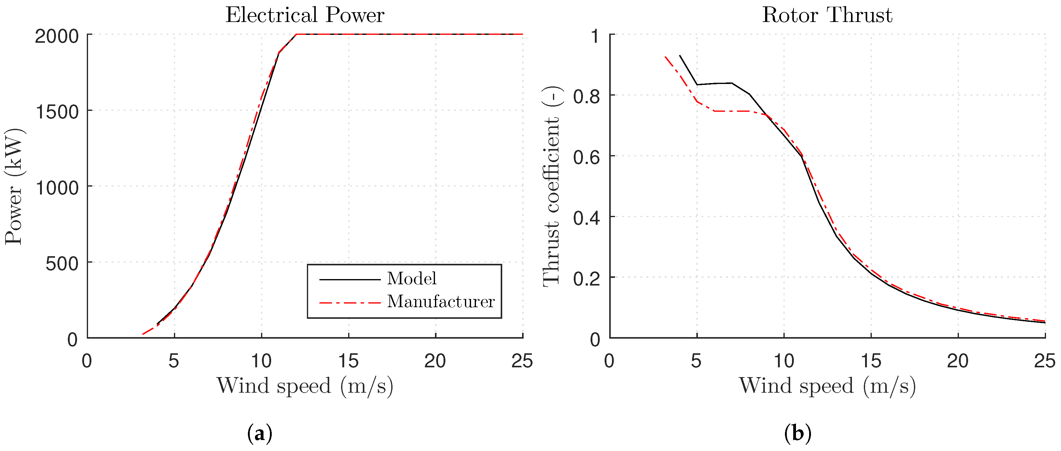
2.1. Wind Turbine Model
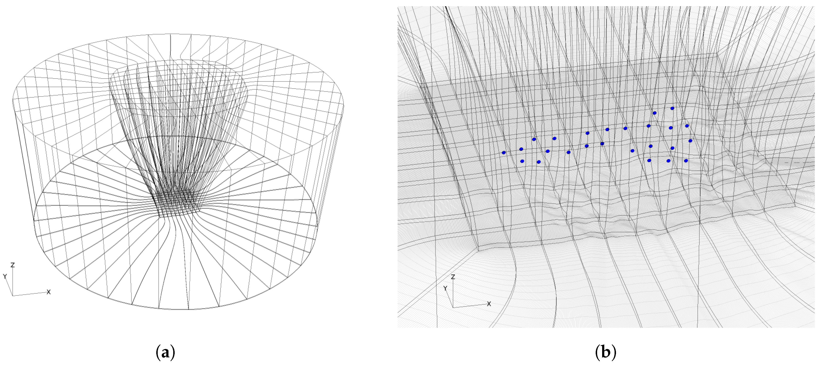
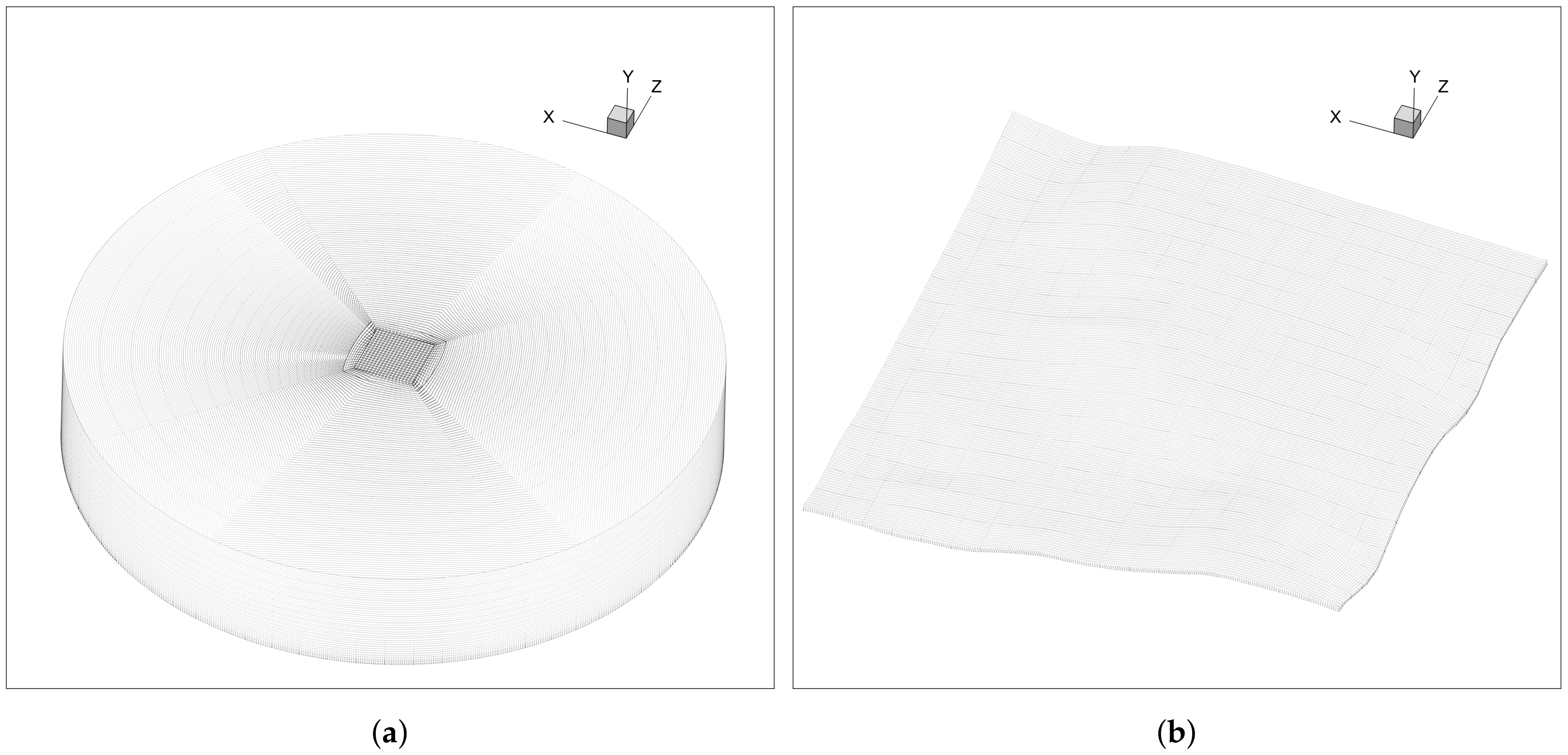
2.2. Actuator Disc Reynolds-Averaged Navier–Stokes Simulation
2.3. Actuator Line Large-Eddy Simulation
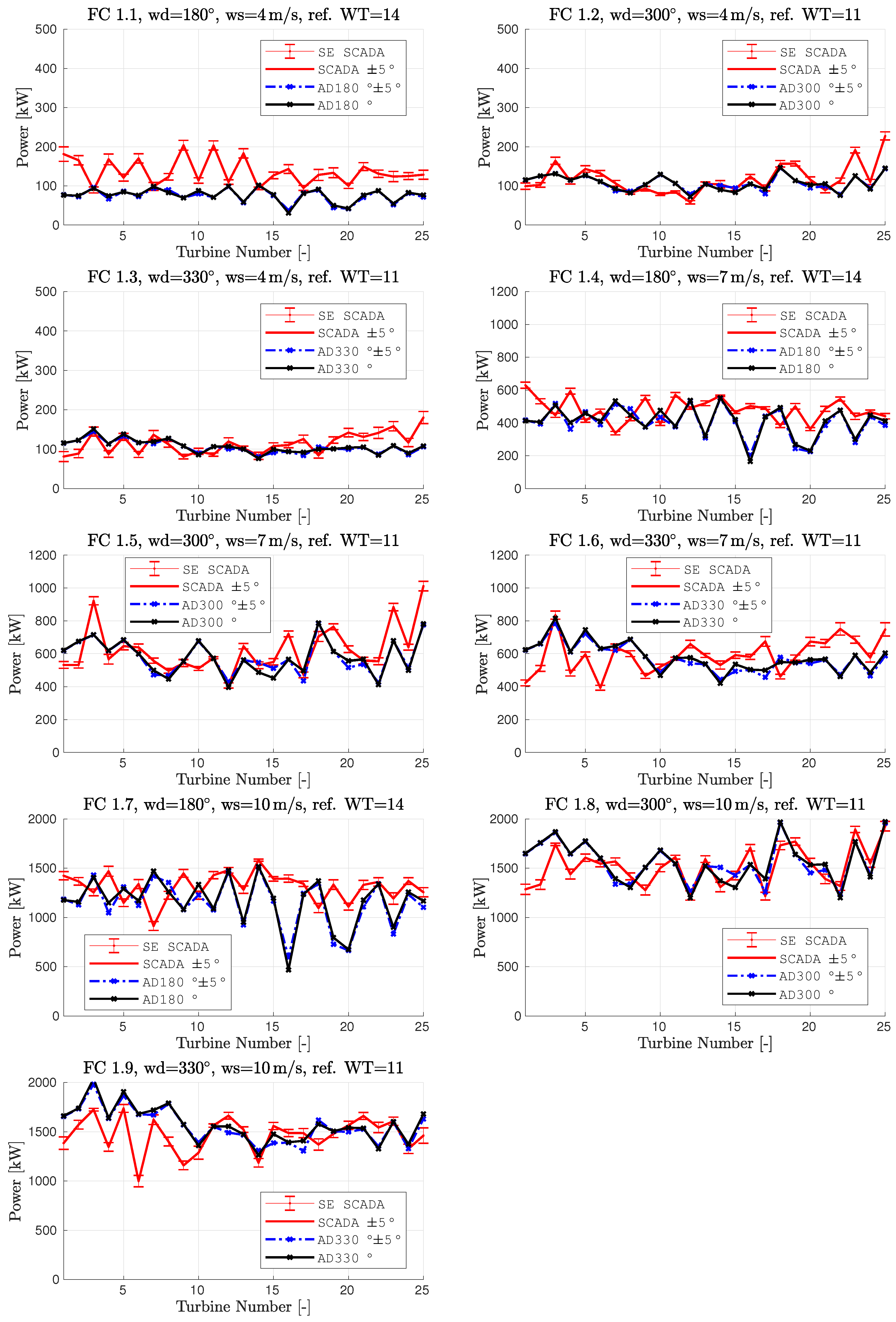
2.4. Flow Cases
3. Results
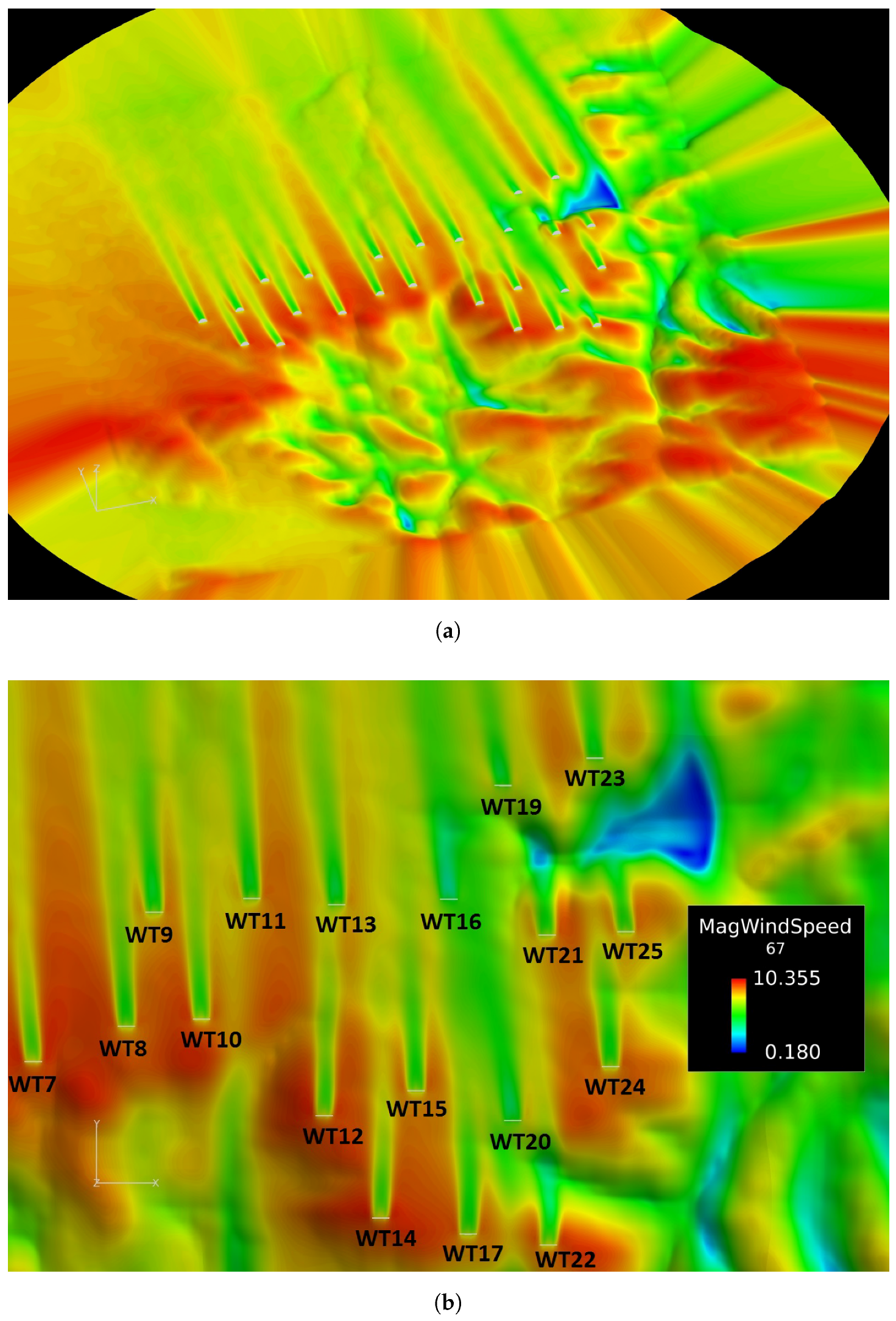
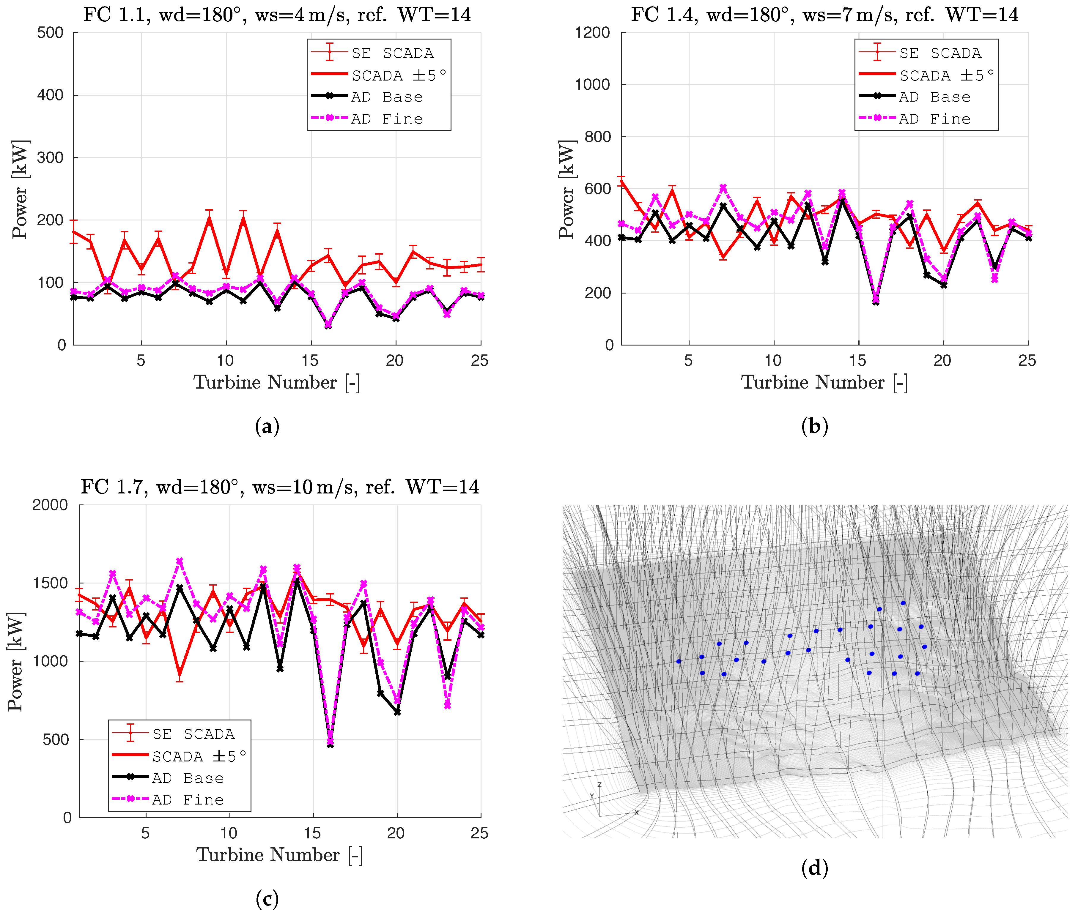
3.1. Actuator Disc Reynolds-Averaged Navier–Stokes Results
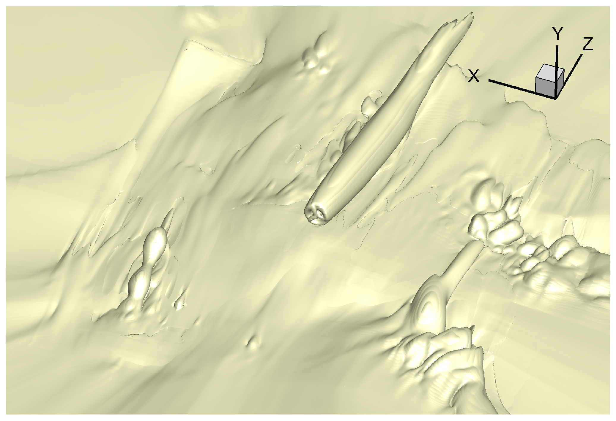
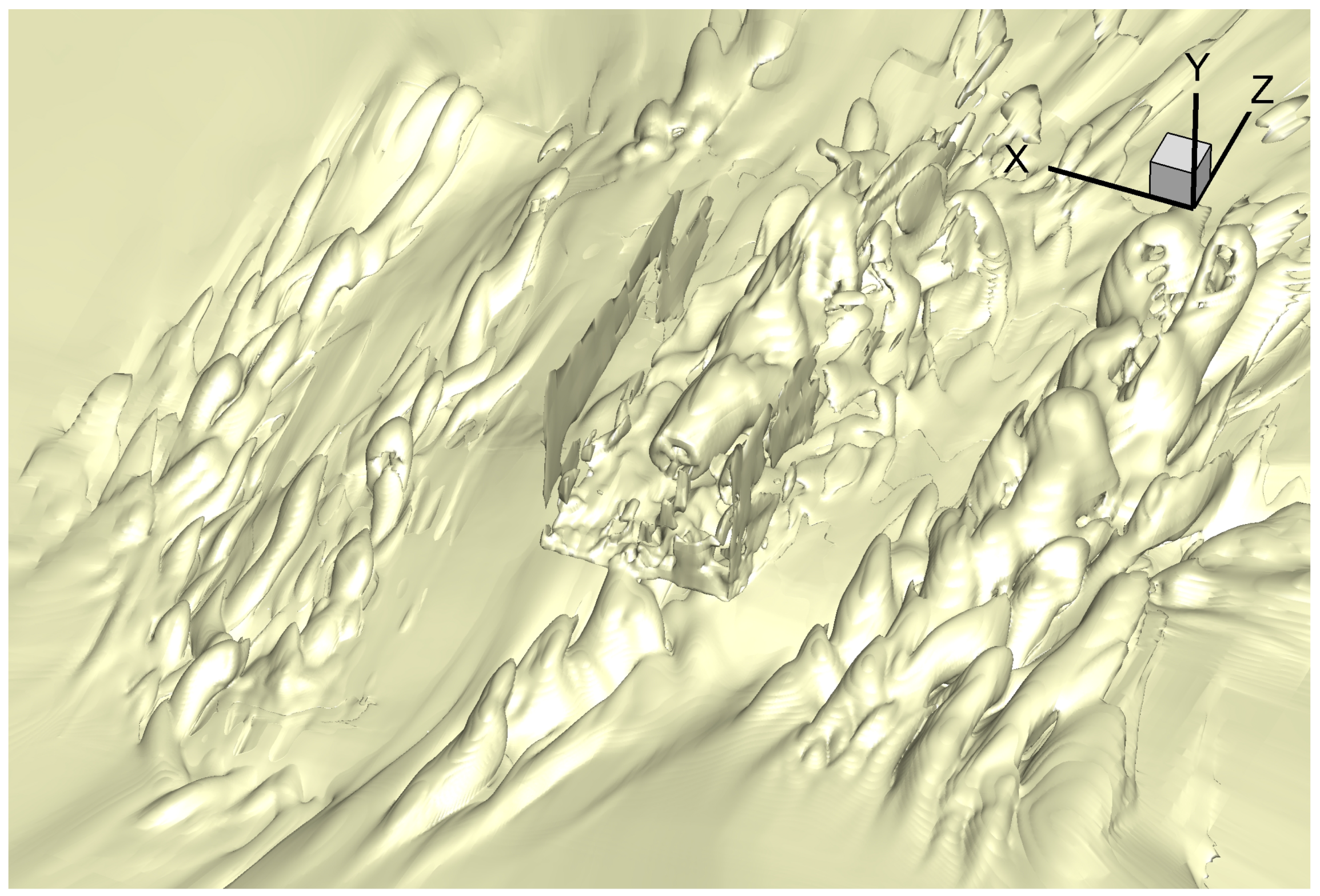
3.2. Actuator Line Large-Eddy Simulation Results
4. Conclusions
Author Contributions
Funding
Acknowledgments
Conflicts of Interest
Abbreviations
| AD | actuator disc |
| AL | actuator line |
| CFD | computational fluid dynamics |
| CSIC | China Shipbuilding Industry Corporation |
| DES | delayed-detached-eddy simulation |
| FC1/FC2 | flow case 1, flow case 2 |
| HZ | Haizhuang |
| LES | large-eddy simulation |
| MW | megawatt |
| RANS | Reynolds-Averaged Navier–Stokes |
| RPM | revolutions per minute |
| SCADA | supervisory control and data acquisition |
| SE | standard error |
| SGS | sub-grid scale |
| STD | standard deviation |
| wd | wind direction |
| ws | wind speed |
| WT(s) | wind turbine(s) |
References
- International Renewable Energy Agency. Renewable Power Generation Costs in 2017; Technical Report; IRENA: Abu Dhabi, UAE, 2018; ISBN 978-92-9260-040-2. [Google Scholar]
- Storey, R.C.; Norris, S.E.; Stol, K.A.; Cater, J.E. Large eddy simulation of dynamically controlled wind turbines in an offshore environment. Wind Energy 2013, 16, 845–864. [Google Scholar] [CrossRef]
- Van der Laan, M.P.; Sørensen, N.N.; Réthoré, P.E.; Mann, J.; Kelly, M.C.; Troldborg, N. The k-ε-fP model applied to double wind turbine wakes using different actuator disk force methods. Wind Energy 2015, 18, 2223–2240. [Google Scholar] [CrossRef]
- Makridis, A.; Chick, J. Validation of a CFD model of wind turbine wakes with terrain effects. J. Wind Eng. Ind. Aerodyn. 2013, 123, 12–29. [Google Scholar] [CrossRef]
- Schulz, C.; Klein, L.; Weihing, P.; Lutz, T.; Krämer, E. CFD Studies on Wind Turbines in Complex Terrain under Atmospheric Inflow Conditions. J. Phys. Conf. Ser. 2014, 524, 012134. [Google Scholar] [CrossRef]
- Schulz, C.; Klein, L.; Weihing, P.; Lutz, T. Investigations into the Interaction of a Wind Turbine with Atmospheric Turbulence in Complex Terrain. J. Phys. Conf. Ser. 2016, 753, 032016. [Google Scholar] [CrossRef]
- Tabib, M.; Rasheed, A.; Kvamsdal, T. LES and RANS simulation of onshore Bessaker wind farm: Analysing terrain and wake effects on wind farm performance. J. Phys. Conf. Ser. 2015, 625, 012032. [Google Scholar] [CrossRef]
- Tabib, M.; Rasheed, A.; Fuchs, F. Analyzing complex wake-terrain interactions and its implications on wind-farm performance. J. Phys. Conf. Ser. 2016, 753, 032063. [Google Scholar] [CrossRef]
- Castellani, F.; Astolfi, D.; Mana, M.; Piccioni, E.; Becchetti, M.; Terzi, L. Investigation of terrain and wake effects on the performance of wind farms in complex terrain using numerical and experimental data. Wind Energy 2017, 20, 1277–1289. [Google Scholar]
- Sørensen, J.N.; Mikkelsen, R.F.; Henningson, D.S.; Ivanell, S.; Sarmast, S.; Andersen, S.J. Simulation of wind turbine wakes using the actuator line technique. Philos. Trans. Ser. A Math. Phys. Eng. Sci. 2015, 373, 20140071. [Google Scholar] [CrossRef] [PubMed]
- Sørensen, N.N. General Purpose Flow Solver Applied to Flow over Hills. Ph.D. Thesis, Technical University of Denmark, Roskilde, Denmark, 1995. [Google Scholar]
- Michelsen, J.A. Basis3D—A Platform for Development of Multiblock PDE Solvers; Technical Report; Technical University of Denmark: Roskilde, Denmark, 1992. [Google Scholar]
- Réthoré, P.E.; van der Laan, P.; Troldborg, N.; Zahle, F.; Sørensen, N.N. Verification and validation of an actuator disc model. Wind Energy 2014, 17, 919–937. [Google Scholar] [CrossRef]
- Sørensen, J.N.; Shen, W.Z. Numerical Modeling of Wind Turbine Wakes. J. Fluids Eng. 2002, 124, 393–399. [Google Scholar] [CrossRef]
- Ramos-García, N.; Sørensen, J.N.; Shen, W.Z. A strong viscous-inviscid interaction model for rotating airfoils. Wind Energy 2014, 17, 1957–1984. [Google Scholar] [CrossRef]
- Han, X.; Liu, D.; Xu, C.; Shen, W.Z. Atmospheric stability and topography effects on wind turbine performance and wake properties in complex terrain. Renew. Energy 2018, 126, 640–651. [Google Scholar] [CrossRef]
- Van der Laan, M.P.; Sørensen, N.N.; Réthoré, P.E.; Mann, J.; Kelly, M.C.; Troldborg, N.; Schepers, J.G.; Machefaux, E. An improved k-ε model applied to a wind turbine wake in atmospheric turbulence. Wind Energy 2015, 18, 889–907. [Google Scholar] [CrossRef]
- Andersen, S.J.; Sørensen, J.N.; Mikkelsen, R. Simulation of the inherent turbulence and wake interaction inside an infinitely long row of wind turbines. J. Turbul. 2013, 14, 1–24. [Google Scholar] [CrossRef]
- Mann, J. The spatial structure of neutral atmospheric surface-layer turbulence. J. Fluid Mech. 1994, 273, 141–168. [Google Scholar] [CrossRef]
- Mann, J. Wind field simulation. Probab. Eng. Mech. 1998, 13, 269–282. [Google Scholar] [CrossRef]


| Name | CSIC HZ93-2.0MW |
|---|---|
| Diameter | 93 m |
| Power rating | 2.0 MW |
| Hub height | 67 m |
| Power control | Variable speed, collective blade pitch control |
| FC1 | Sector | Wind Speed, h = 67 m | Reference Wind Speed | Reference Wind Direction |
|---|---|---|---|---|
| 1.1 | 180 ± 5 | 4 ± 1 m/s | WT14, h = 67 m | M3, h = 70 m |
| 1.2 | 300 ± 5 | 4 ± 1 m/s | WT11, h = 67 m | M1, h = 70 m |
| 1.3 | 330 ± 5 | 4 ± 1 m/s | WT11, h = 67 m | M1, h = 70 m |
| 1.4 | 180 ± 5 | 7 ± 1 m/s | WT14, h = 67 m | M3, h = 70 m |
| 1.5 | 300 ± 5 | 7 ± 1 m/s | WT11, h = 67 m | M1, h = 70 m |
| 1.6 | 330 ± 5 | 7 ± 1 m/s | WT11, h = 67 m | M1, h = 70 m |
| 1.7 | 180 ± 5 | 10 ± 1 m/s | WT14, h = 67 m | M3, h = 70 m |
| 1.8 | 300 ± 5 | 10 ± 1 m/s | WT11, h = 67 m | M1, h = 70 m |
| 1.9 | 330 ± 5 | 10 ± 1 m/s | WT11, h = 67 m | M1, h = 70 m |
| FC2 | Sector | Wind Speed, h = 67 m | Reference Wind Speed | Reference Wind Direction |
|---|---|---|---|---|
| 2.1 | 180 ± 5 | 4 ± 1 m/s | M3, h = 70 m | M3, h = 70 m |
| 2.2 | 180 ± 5 | 7 ± 1 m/s | M3, h = 70 m | M3, h = 70 m |
| 2.3 | 0 ± 5 | 4 ± 1 m/s | M1, h = 70 m | M1, h = 70 m |
| 2.4 | 0 ± 5 | 7 ± 1 m/s | M1, h = 70 m | M1, h = 70 m |
| FC1 | 1.1 | 1.2 | 1.3 | 1.4 | 1.5 | 1.6 | 1.7 | 1.8 | 1.9 |
|---|---|---|---|---|---|---|---|---|---|
| Turning angle (degrees) | 4.28 | 1.29 | 4.28 | 1.29 | 4.28 | 1.28 | |||
| Speed-up (-) | 1.25 | 1.12 | 1.13 | 1.25 | 1.12 | 1.13 | 1.25 | 1.12 | 1.13 |
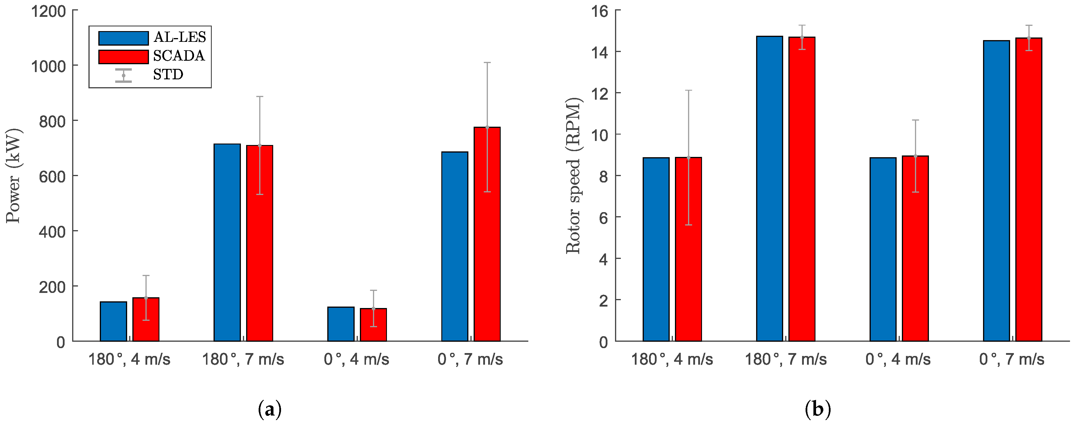
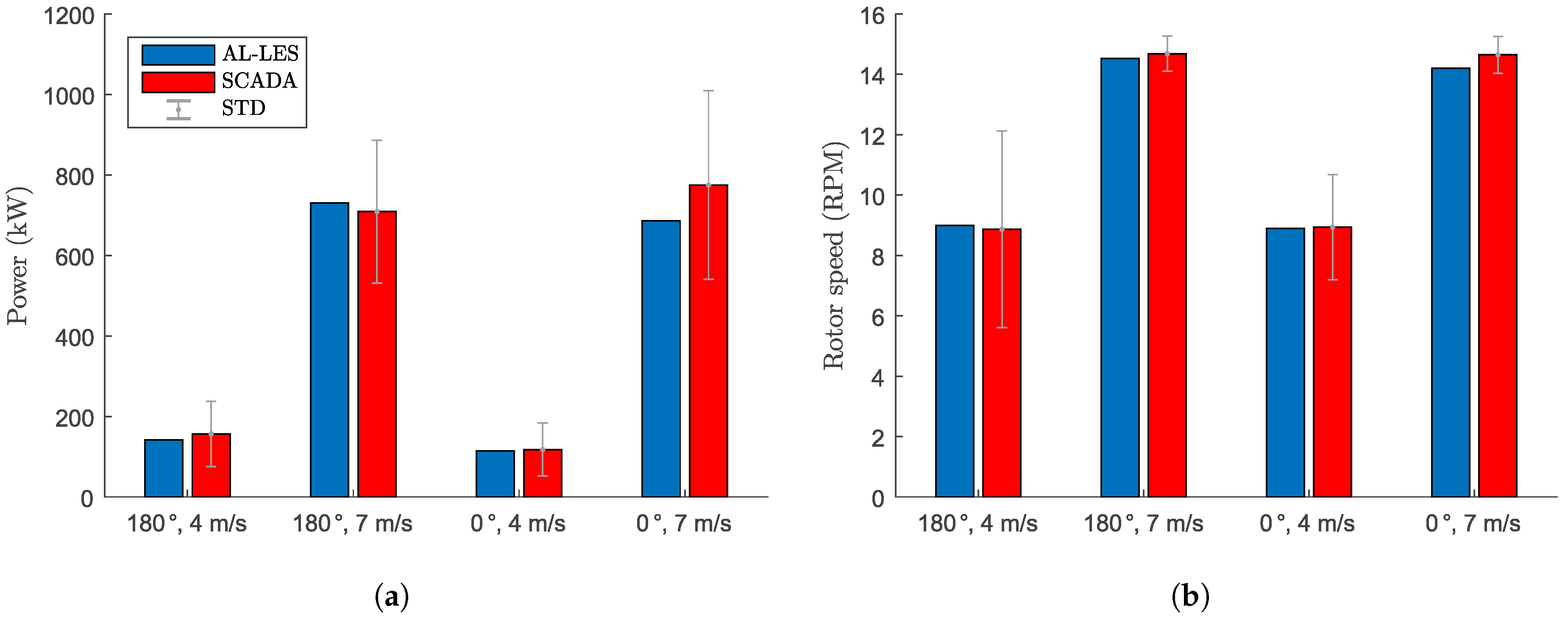
| AL-LES (Black), Measured (Blue), % diff. (Purple) | 180, 4 m/s | STD | 180, 7 m/s | STD | 0, 4 m/s | STD | 0, 7 m/s | STD |
|---|---|---|---|---|---|---|---|---|
| 142.0 | 714.3 | 123.1 | 685.1 | |||||
| Power (kW) | 156.6 | 81.2 | 709.0 | 177.4 | 117.8 | 65.8 | 775.0 | 234.3 |
| −9.32% | 0.75% | 4.50% | −11.60% | |||||
| 8.860 | 14.720 | 8.860 | 14.520 | |||||
| Rotor speed (RPM) | 8.868 | 3.253 | 14.680 | 0.587 | 8.940 | 1.742 | 14.646 | 0.613 |
| −0.08% | 0.27% | −0.89% | −0.86% | |||||
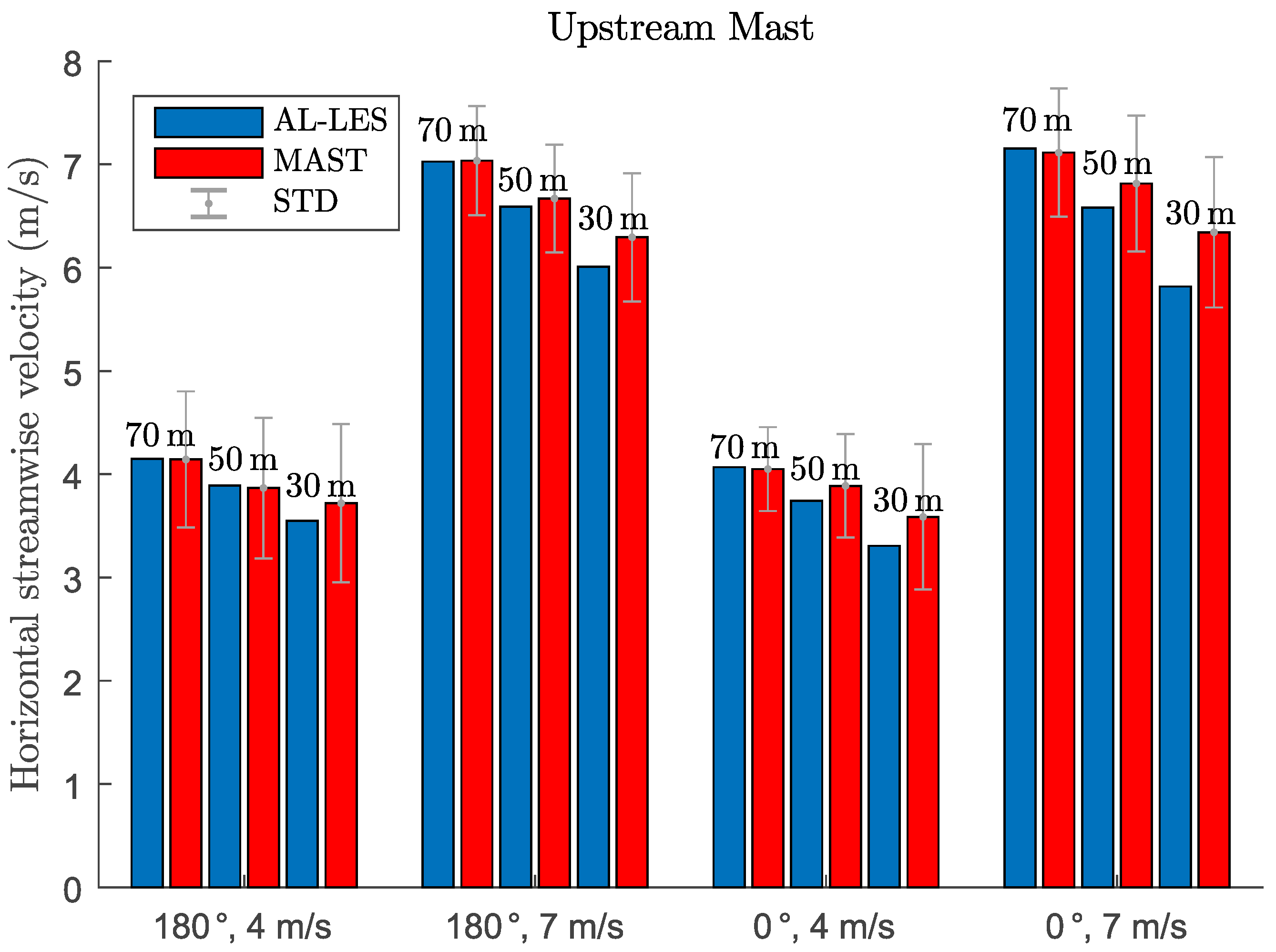
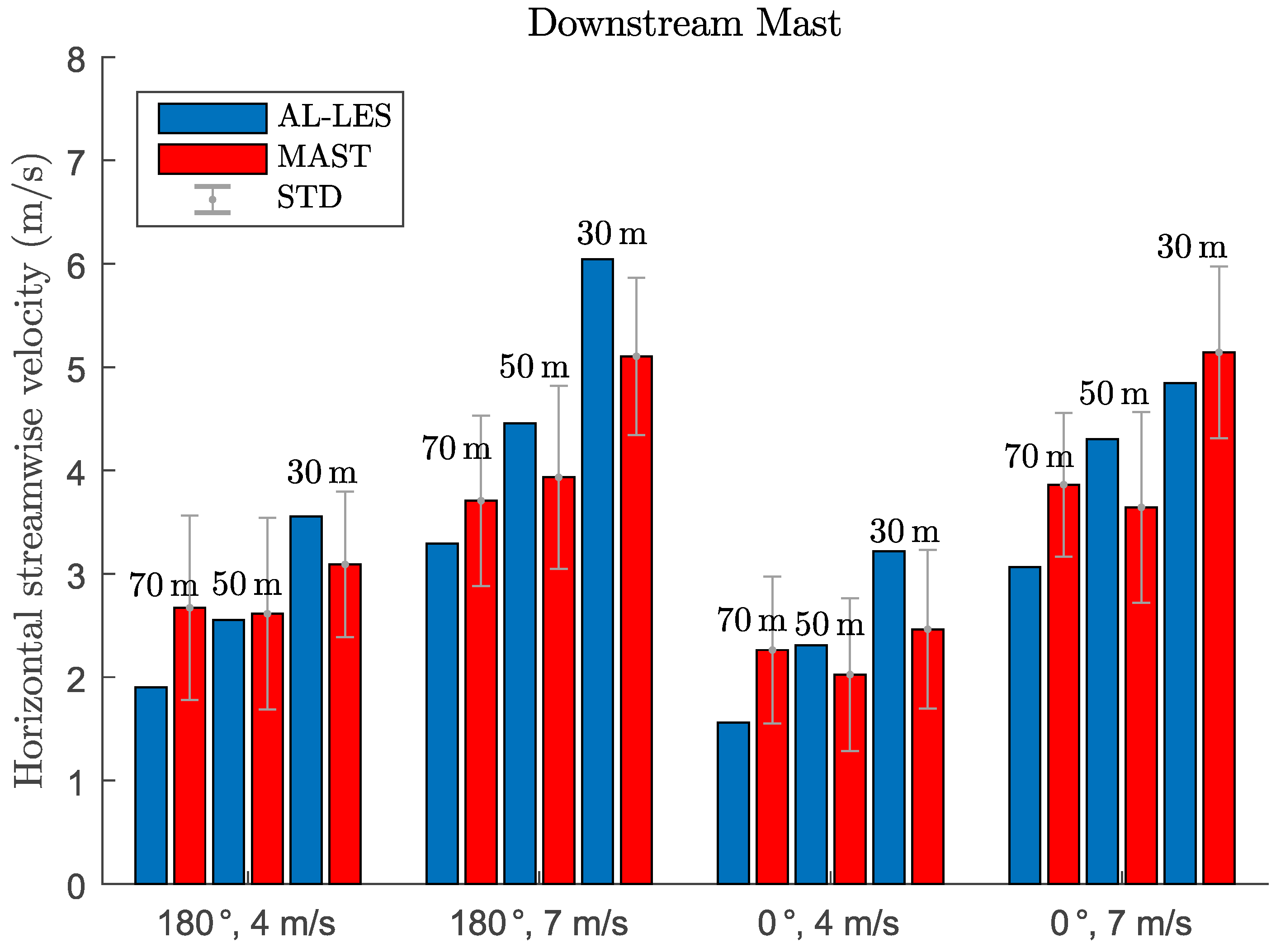
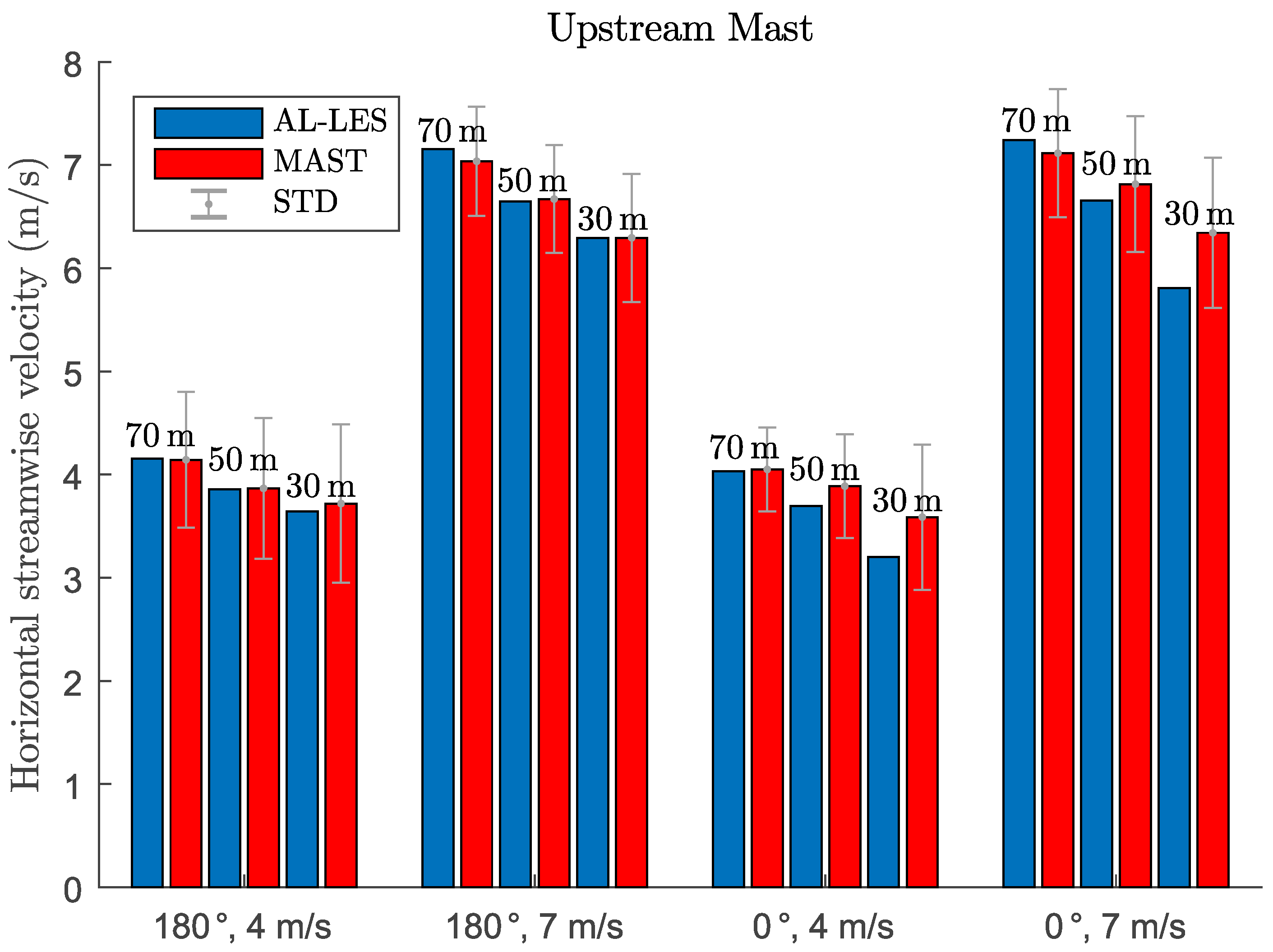
| Streamwise vel. (m/s) | 4.149 | 7.027 | 1.560 | 3.066 | ||||
| @ 70 m | 4.143 | 0.659 | 7.036 | 0.528 | 2.263 | 0.894 | 3.862 | 0.824 |
| M3 | 0.15% | −0.12% | −31.06% | −20.61% | ||||
| Streamwise vel. (m/s) | 3.891 | 6.590 | 2.308 | 4.302 | ||||
| @ 50 m | 3.867 | 0.681 | 6.669 | 0.523 | 2.025 | 0.927 | 3.643 | 0.887 |
| M3 | 0.62% | −1.19% | 13.98% | 18.10% | ||||
| Streamwise vel. (m/s) | 3.547 | 6.009 | 3.217 | 4.845 | ||||
| @ 30 m | 3.719 | 0.766 | 6.294 | 0.621 | 2.463 | 0.705 | 5.143 | 0.761 |
| M3 | −4.62% | −4.54% | 30.57% | −5.80% | ||||
| Streamwise vel. (m/s) | 1.902 | 3.294 | 4.068 | 7.155 | ||||
| @ 70 m | 2.671 | 0.712 | 3.707 | 0.695 | 4.050 | 0.406 | 7.114 | 0.620 |
| M1 | −28.81% | −11.13% | 0.46% | 0.58% | ||||
| Streamwise vel. (m/s) | 2.554 | 4.457 | 3.741 | 6.582 | ||||
| @ 50 m | 2.614 | 0.738 | 3.933 | 0.923 | 3.888 | 0.501 | 6.814 | 0.658 |
| M1 | −2.30% | 13.30% | −3.76% | −3.42% | ||||
| Streamwise vel. (m/s) | 3.554 | 6.042 | 3.306 | 5.818 | ||||
| @ 30 m | 3.090 | 0.767 | 5.104 | 0.830 | 3.588 | 0.704 | 6.343 | 0.728 |
| M1 | 15.01% | 18.38% | −7.85% | −8.28% |
| AL-LES (Black), Measured (Blue), % diff. (Purple) | 180, 4 m/s | STD | 180, 7 m/s | STD | 0, 4 m/s | STD | 0, 7 m/s | STD |
|---|---|---|---|---|---|---|---|---|
| 141.6 | 730.3 | 114.2 | 686.5 | |||||
| Power (kW) | 156.6 | 81.2 | 709.0 | 177.4 | 117.8 | 65.8 | 775.0 | 234.3 |
| −9.59% | 3.01% | −3.05% | −11.42% | |||||
| 8.988 | 14.523 | 8.899 | 14.207 | |||||
| Rotor speed (RPM) | 8.868 | 3.253 | 14.684 | 0.587 | 8.938 | 1.742 | 14.646 | 0.613 |
| 1.36% | −1.10% | −0.44% | −3.00% | |||||
| Streamwise vel. (m/s) | 4.152 | 7.156 | 1.623 | 3.538 | ||||
| @ 70 m | 4.143 | 0.659 | 7.036 | 0.528 | 2.263 | 0.894 | 3.862 | 0.824 |
| M3 | 0.23% | 1.70% | −28.28% | −8.38% | ||||
| Streamwise vel. (m/s) | 3.858 | 6.648 | 1.970 | 4.151 | ||||
| @ 50 m | 3.867 | 0.681 | 6.669 | 0.523 | 2.025 | 0.927 | 3.643 | 0.887 |
| M3 | −0.22% | −0.33% | −2.71% | 13.94% | ||||
| Streamwise vel. (m/s) | 3.644 | 6.291 | 2.914 | 5.484 | ||||
| @ 30 m | 3.719 | 0.766 | 6.294 | 0.621 | 2.463 | 0.705 | 5.143 | 0.761 |
| M3 | −2.01% | −0.06% | 18.34% | 6.63% | ||||
| Streamwise vel. (m/s) | 2.095 | 3.934 | 4.031 | 7.243 | ||||
| @ 70 m | 2.671 | 0.712 | 3.707 | 0.695 | 4.050 | 0.406 | 7.114 | 0.620 |
| M1 | −21.59% | 6.12% | −0.47% | 1.81% | ||||
| Streamwise vel. (m/s) | 2.558 | 4.705 | 3.695 | 6.655 | ||||
| @ 50 m | 2.614 | 0.738 | 3.933 | 0.923 | 3.888 | 0.501 | 6.814 | 0.658 |
| M1 | −2.17% | 19.61% | −4.95% | −2.33% | ||||
| Streamwise vel. (m/s) | 3.459 | 6.033 | 3.202 | 5.805 | ||||
| @ 30 m | 3.090 | 0.767 | 5.104 | 0.830 | 3.588 | 0.704 | 6.343 | 0.728 |
| M1 | 11.94% | 18.20% | −10.75% | −8.48% | ||||
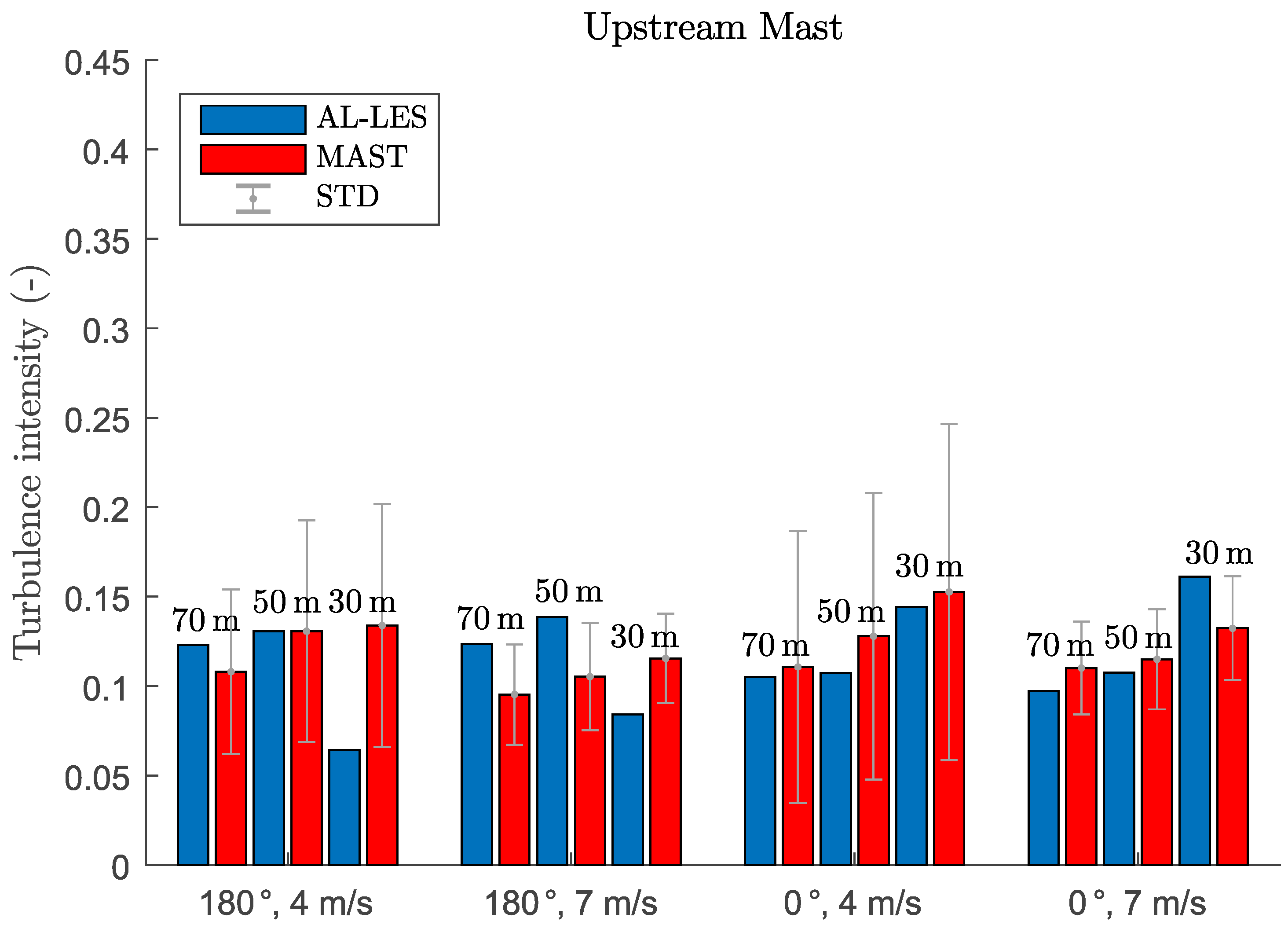
| Turbulence intensity (-) | 0.123 | 0.123 | 0.206 | 0.234 | ||||
| @ 70 m | 0.108 | 0.046 | 0.095 | 0.028 | 0.264 | 0.122 | 0.229 | 0.063 |
| M3 | 13.92% | 29.60% | −22.21% | 2.16% | ||||
| Turbulence intensity (-) | 0.131 | 0.138 | 0.212 | 0.221 | ||||
| @ 50 m | 0.131 | 0.062 | 0.105 | 0.030 | 0.278 | 0.126 | 0.255 | 0.069 |
| M3 | 0.00% | 31.60% | −23.52% | −13.40% | ||||
| Turbulence intensity (-) | 0.064 | 0.084 | 0.185 | 0.185 | ||||
| @ 30 m | 0.134 | 0.068 | 0.115 | 0.025 | 0.271 | 0.096 | 0.242 | 0.041 |
| M3 | −52.06% | −27.08% | −31.72% | −23.53% | ||||
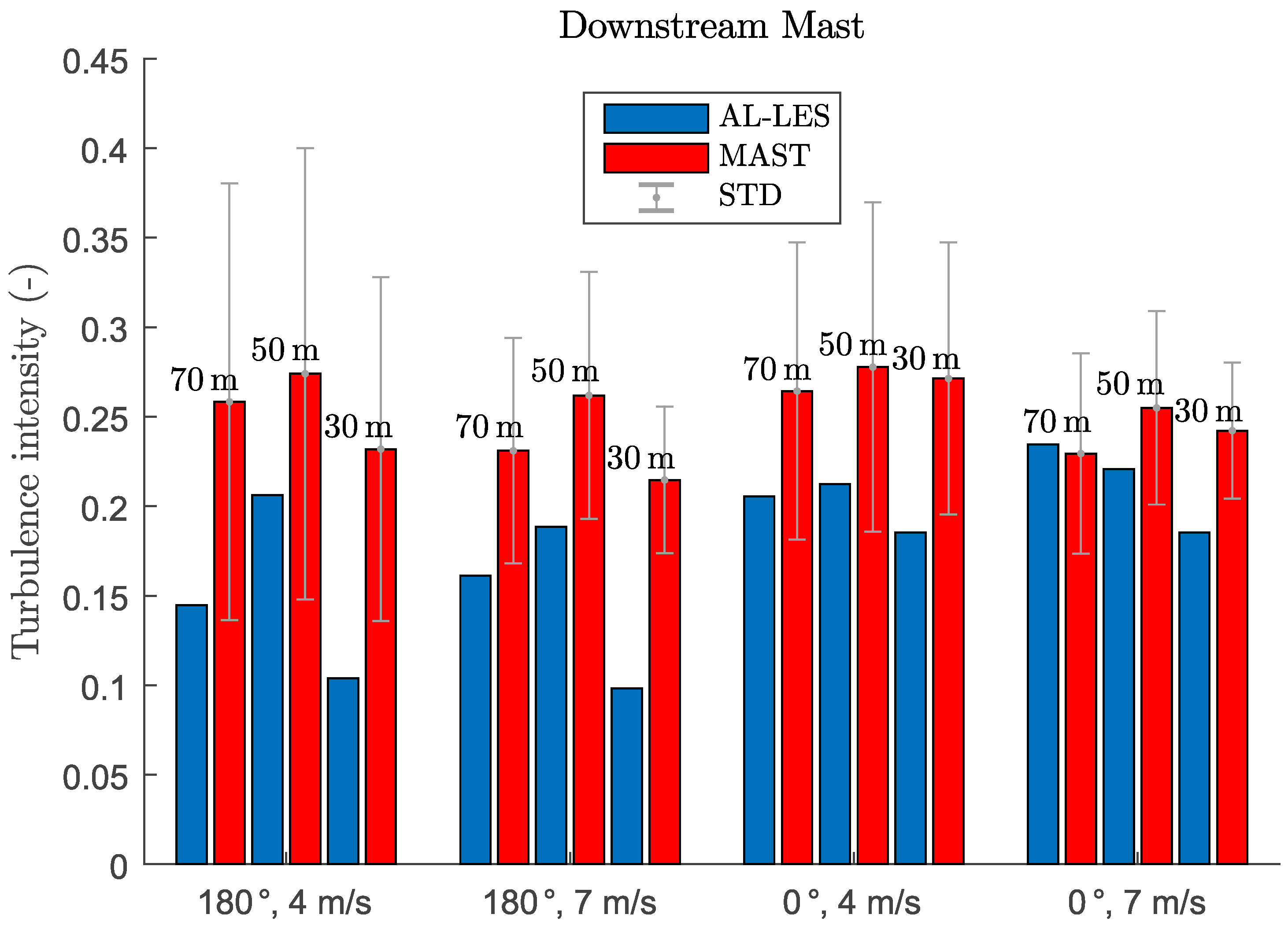
| Turbulence intensity (-) | 0.145 | 0.161 | 0.105 | 0.097 | ||||
| @ 70 m | 0.258 | 0.083 | 0.231 | 0.056 | 0.111 | 0.076 | 0.110 | 0.026 |
| M1 | −43.99% | −30.17% | −5.17% | −11.82% | ||||
| Turbulence intensity (-) | 0.206 | 0.188 | 0.107 | 0.107 | ||||
| @ 50 m | 0.274 | 0.092 | 0.262 | 0.054 | 0.128 | 0.080 | 0.115 | 0.028 |
| M1 | −24.75% | −28.07% | −16.01% | −6.59% | ||||
| Turbulence intensity (-) | 0.104 | 0.098 | 0.144 | 0.161 | ||||
| @ 30 m | 0.232 | 0.076 | 0.215 | 0.038 | 0.153 | 0.094 | 0.132 | 0.029 |
| M1 | −55.23% | −54.23% | −5.51% | 21.74% |
© 2018 by the authors. Licensee MDPI, Basel, Switzerland. This article is an open access article distributed under the terms and conditions of the Creative Commons Attribution (CC BY) license (http://creativecommons.org/licenses/by/4.0/).
Share and Cite
Sessarego, M.; Shen, W.Z.; Van der Laan, M.P.; Hansen, K.S.; Zhu, W.J. CFD Simulations of Flows in a Wind Farm in Complex Terrain and Comparisons to Measurements. Appl. Sci. 2018, 8, 788. https://doi.org/10.3390/app8050788
Sessarego M, Shen WZ, Van der Laan MP, Hansen KS, Zhu WJ. CFD Simulations of Flows in a Wind Farm in Complex Terrain and Comparisons to Measurements. Applied Sciences. 2018; 8(5):788. https://doi.org/10.3390/app8050788
Chicago/Turabian StyleSessarego, Matias, Wen Zhong Shen, Maarten Paul Van der Laan, Kurt Schaldemose Hansen, and Wei Jun Zhu. 2018. "CFD Simulations of Flows in a Wind Farm in Complex Terrain and Comparisons to Measurements" Applied Sciences 8, no. 5: 788. https://doi.org/10.3390/app8050788
APA StyleSessarego, M., Shen, W. Z., Van der Laan, M. P., Hansen, K. S., & Zhu, W. J. (2018). CFD Simulations of Flows in a Wind Farm in Complex Terrain and Comparisons to Measurements. Applied Sciences, 8(5), 788. https://doi.org/10.3390/app8050788