Adaptive Noise Cancellation Based on Time Delay Estimation for Low Frequency Communication

Abstract

Low frequency communication, taking advantage of the features of low frequency electromagnetic signals in near field, is widely used in through-the-earth (TTE) wireless applications. However, the low frequency non-Gaussian noise severely limits the communication performance. In this paper, an adaptive noise cancellation algorithm based on time delay estimation (ANC-TDE) and maximum correntropy criterion (MCC) is proposed. The explicit time delay estimation algorithm based on MCC (MCC-ETDE) is used to estimate the time-varying delay and the noise correlationship between the primary input and reference inputs. With a reference noise selected and time delay compensated, the non-Gaussian noise is canceled by adaptive filter based on MCC. The proposed algorithm is implemented on field programmable gate array (FPGA) and the performance is evaluated by simulation and experiment. As shown in the results, the ANC-TDE algorithm can reduce the complexity of ANC filter and adaptively compensate the varied time delay between the primary input and reference input. With the time delay compensated, the ANC-TDE algorithm has better performance in non-Gaussian noise environment and is more suitable for real-time systems.

1. Introduction

Low frequency (LF) electromagnetic signals are less prone to multipath effect and provide good obstacle penetration in near field [1,2]. Low frequency communication, taking advantage of these features, is an alternative solution for through-the-earth (TTE) wireless applications, such as subsurface wireless data acquisition [3], underground localization [4,5] and magnetic resonance sounding [6]. To achieve two-way communication in long range, there still are many problems to solve. Low frequency signals have great path loss when propagating through the rock, water, and soil [7]. Therefore, huge antennas are used to obtain sufficient radiation gain, probably unsuitable for some applications [8]. In addition, the atmospheric noise mixed to the weak signals limit the signal-to-noise ratio (SNR) at the surface receiver [9]. In this paper, we focus on noise cancellation in low frequency communication.

In the low-frequency radio range, the electromagnetic noise is caused by the natural electrical activity in the atmosphere and man-made electrical disturbances. The atmospheric noise is produced primarily by local and distant thunderstorms. The man-made noise arises from mining machines, transportation vehicles, power generators, transmission lines, etc. [10]. Because of all these factors, the low frequency noise tends to be highly impulsive and cannot be characterized by Gaussian distribution. The low frequency noise which is picked up by narrowband receivers, can be approximated by a symmetric $\alpha$-stable ($S\alpha S$) model [11]. Usually, the receiver consists of multiple antennas, which are used for the direction of arrival (DOA) estimation [12,13]. In some cases, the additive noise can be cancelled from the signal with some reference antennas [6,14,15]. The reference antennas are used to record only noise which is correlated with the noise in the signal [16]. Then the noise can be subtracted from the signal through adaptive noise cancellation, without prior knowledge of signal and communication systems. A popular adaptation technique is the least mean squares (LMS) adaptive algorithm which exploits the second order moments of the error between the desired signal and the filter output [17]. However, in the presence of impulsive of noise, the poor performance of LMS based methods cannot satisfy the requirements of TTE communication systems. To improve the performance, the least mean fourth (LMF) criterion [18] and least mean p-power (LMP) criterion [19] were proposed, using the fourth-order moment or p-order absolute moment of the error as the adaptation cost function. These algorithms are robust in impulsive noise, but the convergence speed and steady-state performance are not good enough [20].

In order to obtain faster convergence and smaller steady-state error, the information theoretic quantities can be used as cost functions to train adaptive systems [21]. There are two families of algorithms: minimum error entropy (MEE) based algorithms and maximum correntropy criterion (MCC) based algorithms. Using entropy of the error signal as a cost function, MEE based algorithms have good robustness and steady-state performance in non-Gaussian and impulsive noise. However, they are quite unsuitable for practical implementation because of their high computational complexity. As a compromise, MCC based algorithms have the robustness comparable to the MEE based algorithms, with similar computational complexity to LMS [22]. As a localized similarity measure, the correntropy places exponentially decreasing weights on impulsive samples.

As shown in Figure 1, to obtain excellent performance with finite-length filters in practical circumstances, a delay $\Delta$ should be inserted into the primary input [23]. Typically, the value of delay $\Delta$ is chosen equal to about half time delay of the adaptive filter. In the practical TTE communication systems, the primary antenna and reference antennas are usually placed in different locations. The noises from different sources have different and time-varying delays between the primary channel and reference channels, resulting in poor noise cancellation performance. To solve this problem, we can estimate the time-varying delays and compensate them by nonlinear processing [24,25]. But the time delay estimation algorithms based on correlation have poor performance in the impulsive noise environment. To suppress the influence of impulsive noise, the explicit time delay estimation (ETDE) algorithm based on MCC (MCC-ETDE) is proposed in [26], and has better performance in indoor near-field electromagnetic ranging system. In the near-field electromagnetic ranging system, the ETDE algorithm is used to estimate the time delay between the electric filed and magnetic field of transmitted signal. The electric and magnetic fields of the signal are correlated. Therefore, the ETDE algorithm can converge to true time delay, which is used to measure the distance between receiver and transmitter. In the TTE communication systems, some reference inputs are not correlated with the noise in the primary input, which leads to non-convergence of the ETDE algorithm. Therefore, the convergence performance of the ETDE algorithm can be used to measure the correlationship between the reference inputs and the primary input. The reference input will be selected as the reference noise only when the time delay estimation value of this input has the smallest variance. Then the time delay is compensated to improve the noise cancellation performance.

In this paper, an adaptive noise cancellation algorithm based on time delay estimation (ANC-TDE) is proposed and implemented on field programmable gate array (FPGA). The ETDE algorithm not only estimates the time-varying delay but also evaluates the noise correlationship between the primary channel and reference channels. The reference input will be selected as the reference noise only when the time delay value of this input has the smallest variance. Then the time delay is compensated to make sure that the delay between primary input and inference input is almost half the time delay of the adaptive filter. At last, the noise is removed from primary input by adaptive noise canceller based on MCC. The performance of the proposed adaptive noise cancellation algorithm is evaluated by simulation and experiment. As shown in the results, the MCC-ETDE algorithm can converge to the true time delay with small variance in the impulsive noise when the reference noise is correlated to the noise in the primary input. With the time delay compensated, the proposed ANC-TDE algorithm can reduce the impulsive noise, and provide better performance. With the filter length shortened, the proposed ANC-TDE algorithm can reduce the complexity of the ANC filter and is suitable for real-time systems.

In summary, our main contributions are as follows:

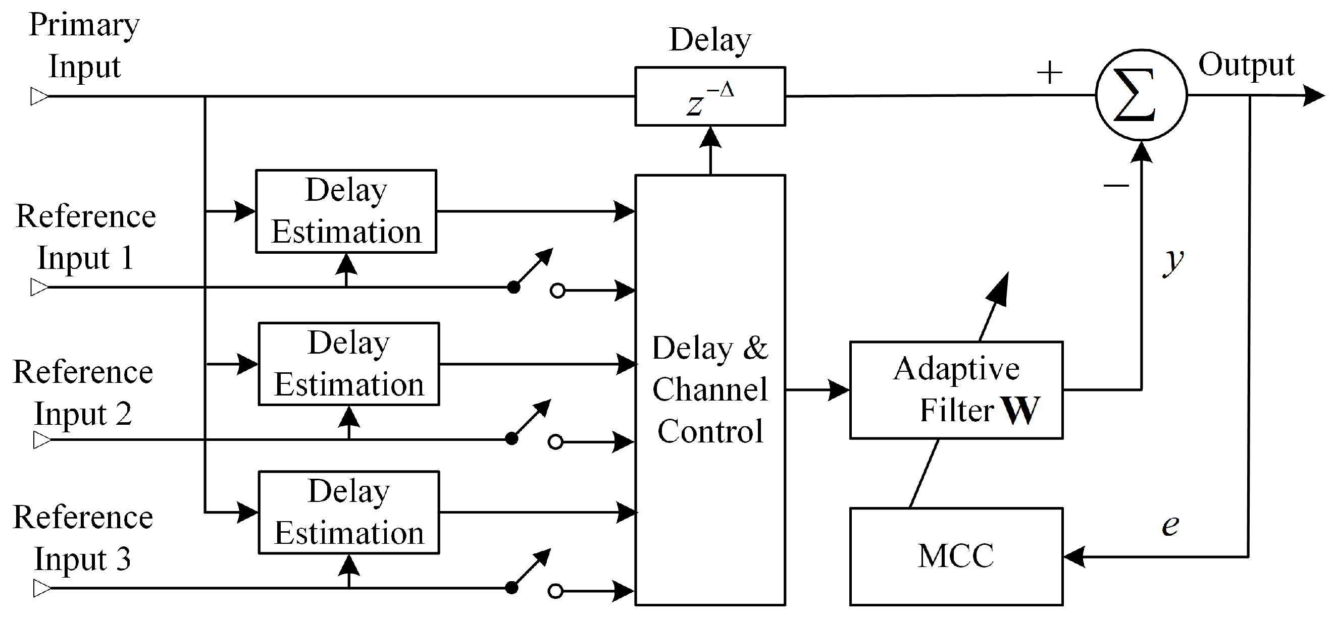
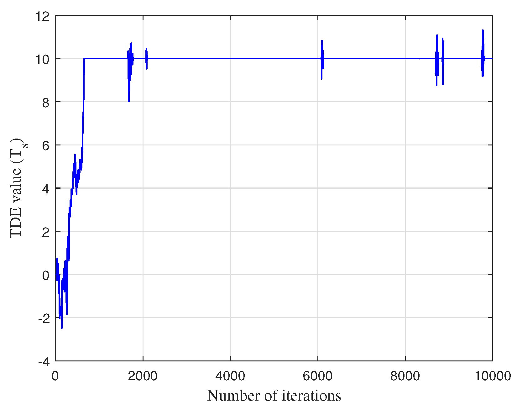
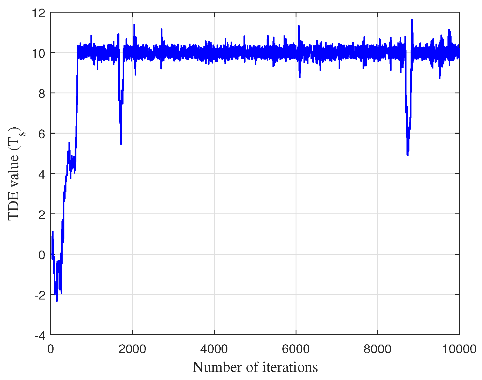
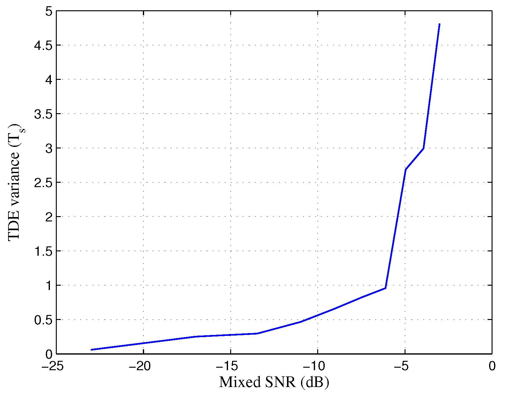
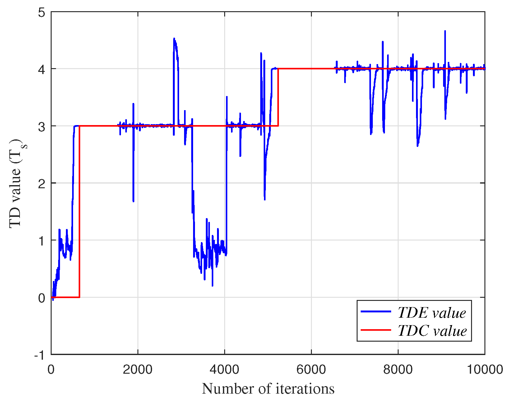
• An adaptive noise cancellation algorithm is proposed based on time delay estimation. The convergence performance of the ETDE algorithm is used to measure the correlationship between the reference inputs and the primary input. The reference input will be selected as the reference noise only when the time delay estimation value of this input has the smallest variance.
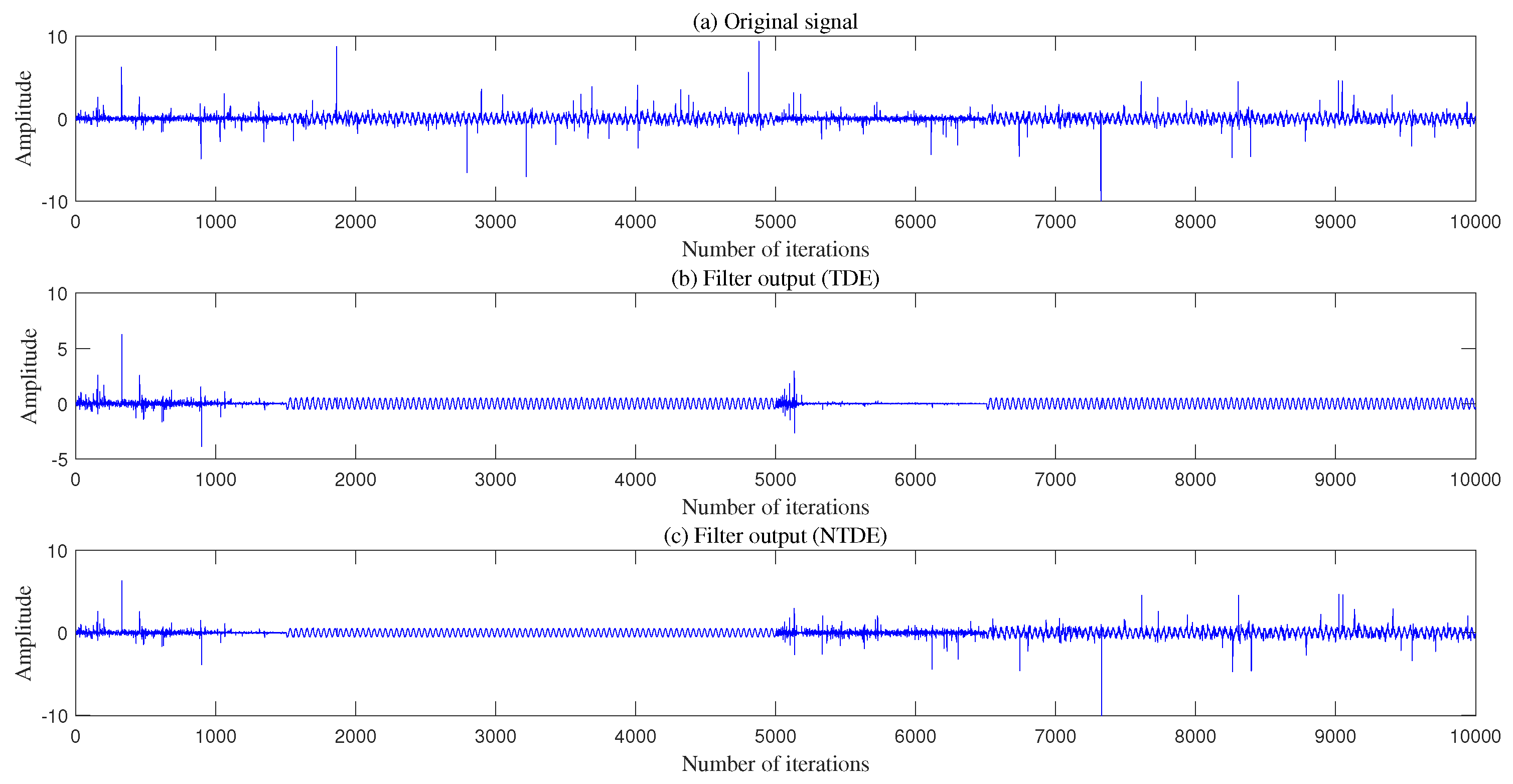
• When the reference noise is determined, the time delay between primary input and inference noise is compensated according to the time delay estimation results. After compensation, the value of delay $\Delta$ is equal to about half time delay of the adaptive filter and the adaptive filter can obtain best noise cancellation performance.
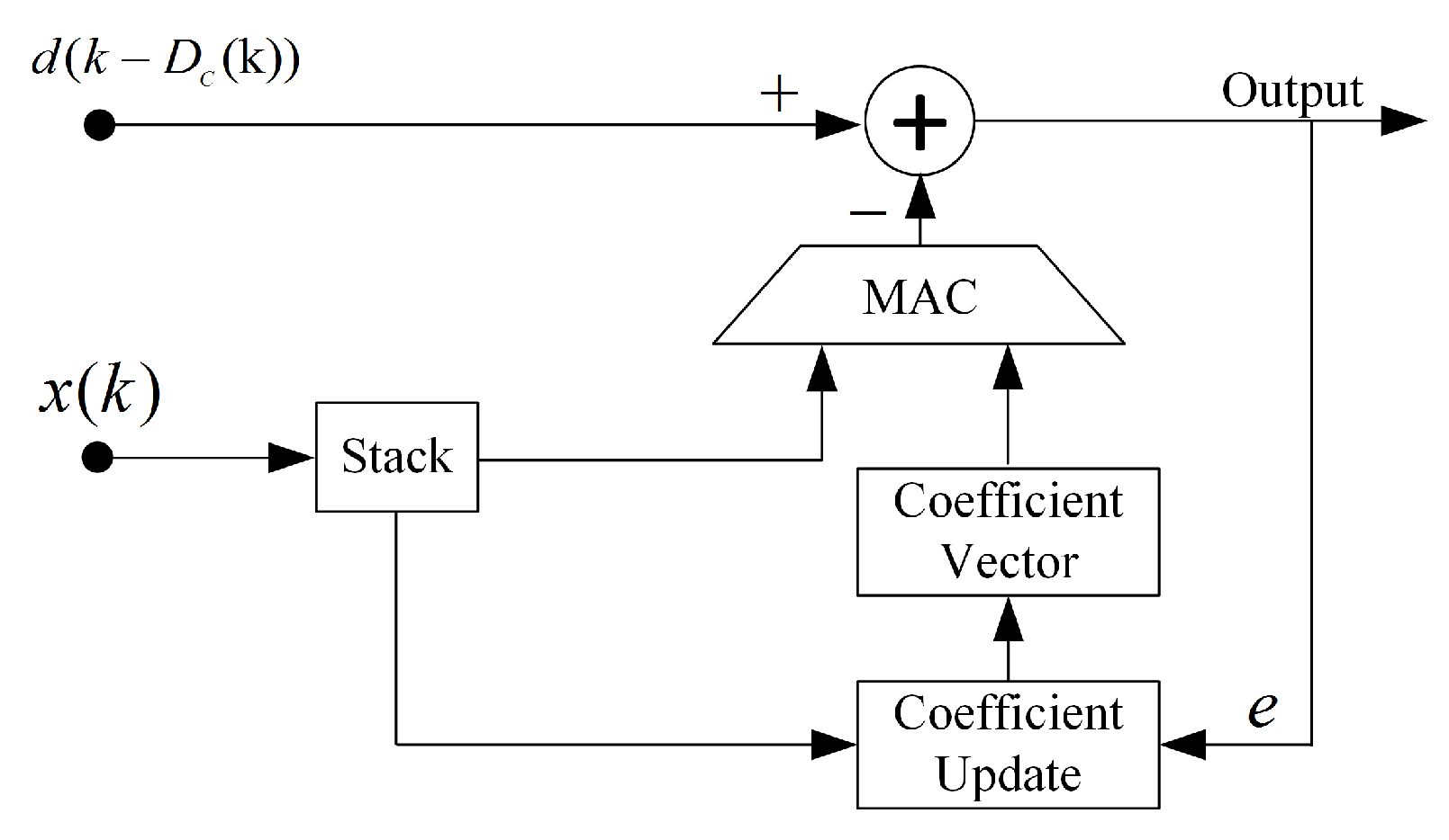
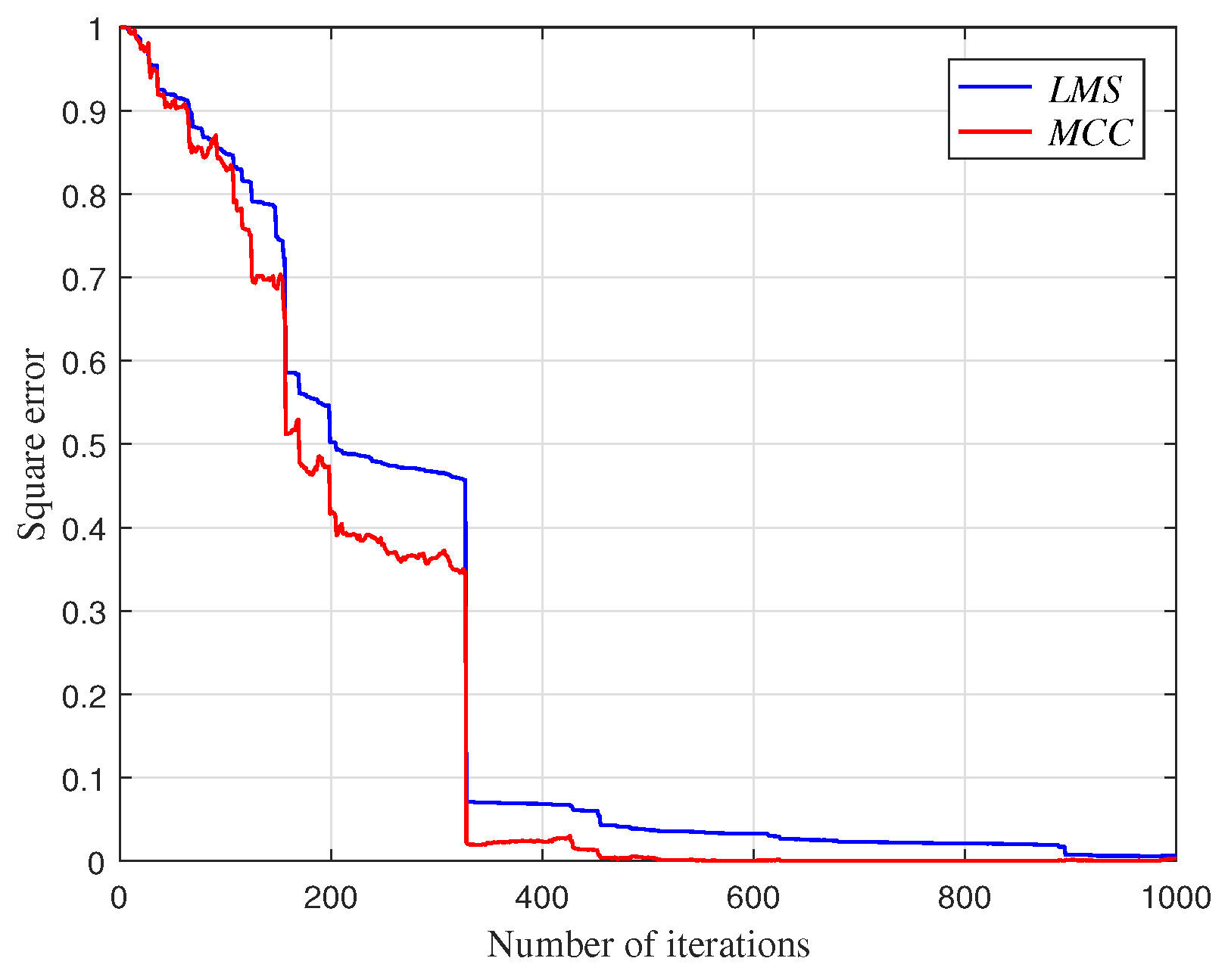
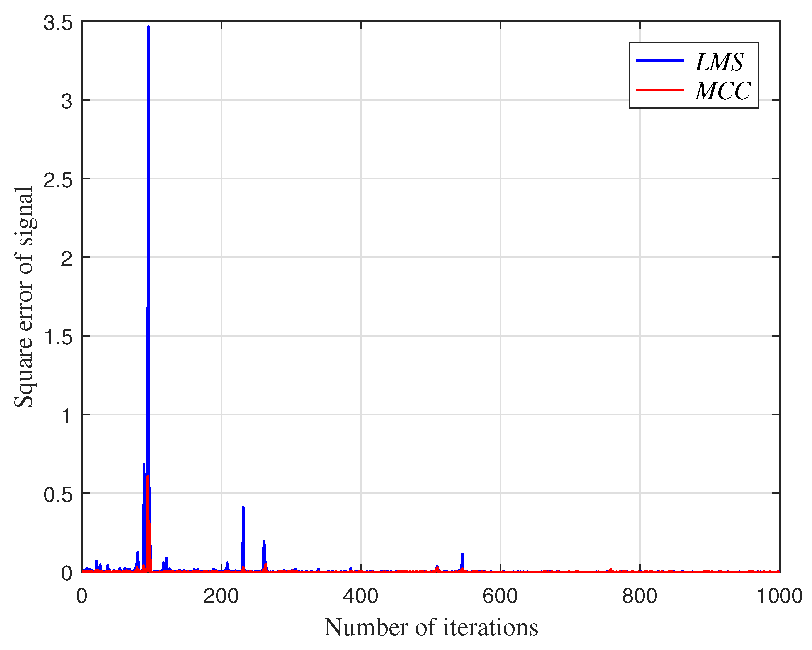
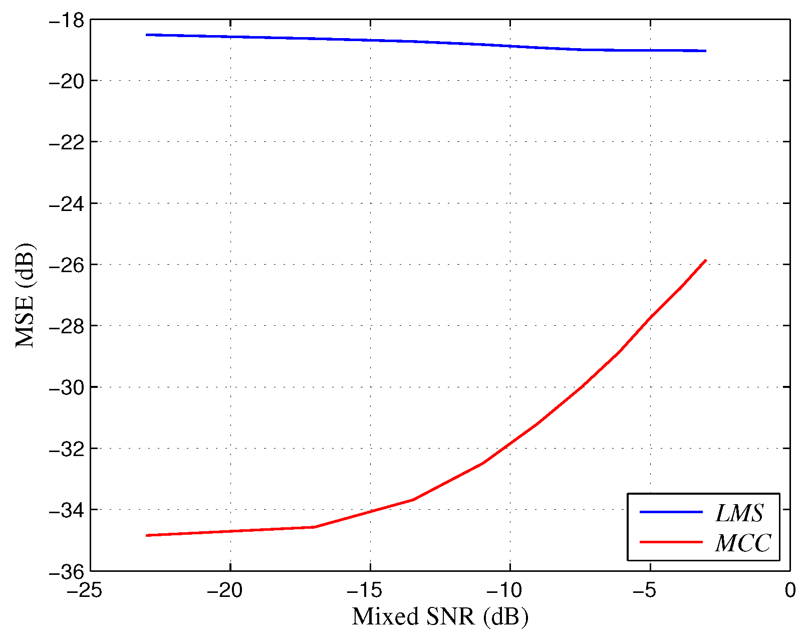
• The adaptive filter is designed based on MCC, which can improve the noise cancellation performance in the impulsive noise environment.
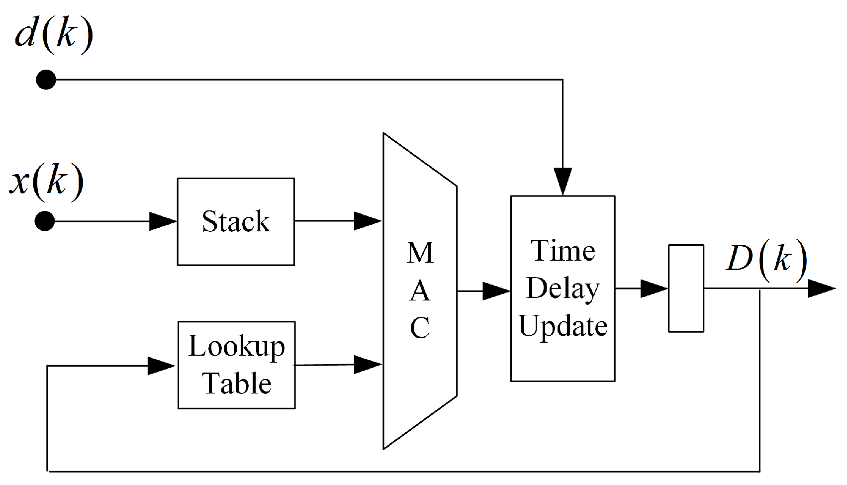
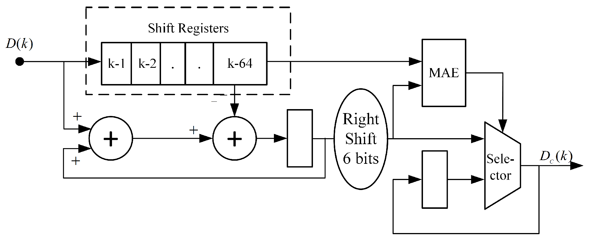
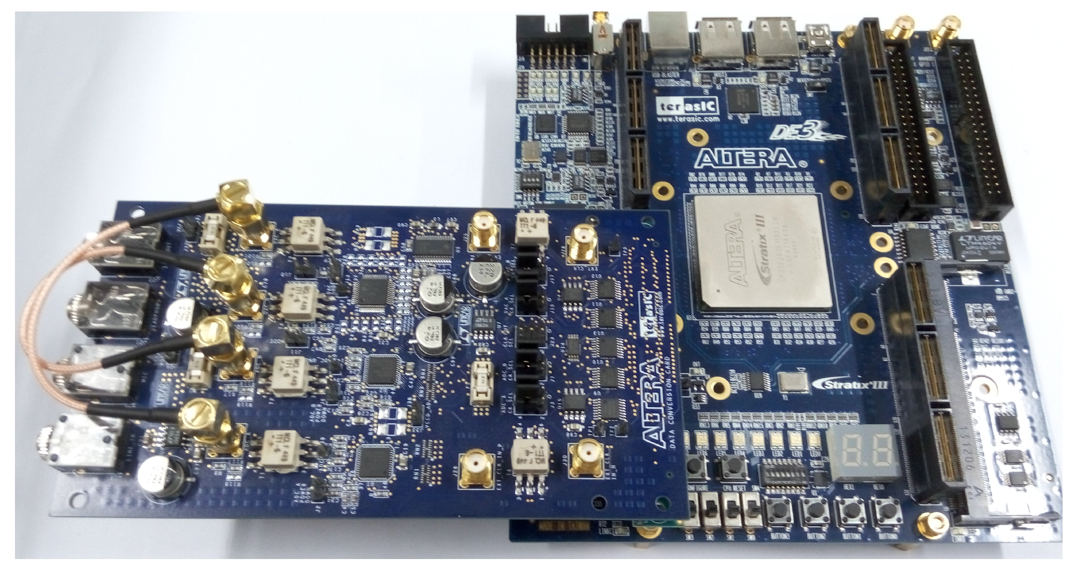
• In order to filter out the correlated noise in real time, the proposed algorithm is implemented on FPGA, which includes three modules: time delay estimation module, delay and channel control module, and noise cancellation module.

The remainder of this paper is organized as follows. Section 2 describes the proposed adaptive noise cancellation algorithm based on MCC. Section 3 details the FPGA implementation of the proposed algorithm. Section 4 evaluates the performance of the proposed system using simulation and experiments. We present conclusions in Section 5.

Notation: Lower-case (resp. Upper-case) bold letters denote column vectors, with $\mathbf{W}\left(k\right)$ being the kth results obtained in the iteration process; $E\left[·\right]$, ${\left(·\right)}^T$, $exp\left(·\right)$, $k_{\sigma }\left(·\right)$ and $G_{\sigma }\left(·\right)$ denote expectation, transpose, natural exponential function, shift-invariant Mercer kernel function with kernel size $\sigma$ and Gaussian kernel function with kernel size $\sigma$, respectively; j denotes the imaginary unit; $\nabla J\left(k\right)$ denotes the gradient of $J\left(k\right)$, while $J\left(k\right)$ denotes the cost function at k moment.

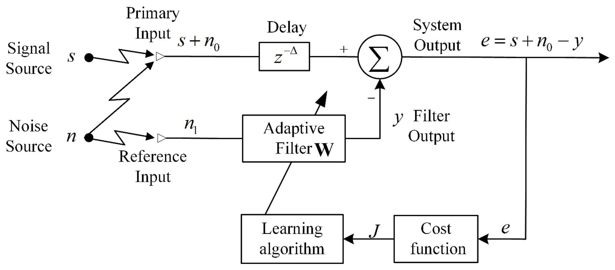
2. Adaptive Noise Cancellation Based on Time Delay Estimation

In most applications, low frequency magnetic signals are used as the communication signals, received by a primary loop antenna. Then the reference noise can be electric field component of noise received by electric antennas at the same position or magnetic field component of noise received by loop antennas at different locations. As shown in Figure 1, suppose that $\mathbf{d}$ is the desired signal at primary input and $\mathbf{x}$ is the noise signal at the reference input. So we get:

$$\mathbf{d}=\mathbf{s}+{\mathbf{n}}_0$$

(1)

$$\mathbf{x}={\mathbf{n}}_1$$

(2)

where, $\mathbf{s}$ is the interesting signal, ${\mathbf{n}}_0$ and ${\mathbf{n}}_1$ are the low frequency correlated noises. The adaptive filter output is obtained by:

$$\mathbf{y}={\mathbf{W}}^T\mathbf{x}$$

(3)

where, $\mathbf{W}$ is the adaptive filter coefficient vector. With appropriate cost function, the additive noise can be subtracted from the primary signal by adaptive noise canceller.

Widely used to model the non-Gaussian signals in brain images [27], power-line communication [28], pattern recognition [29], and so on, the $\alpha$-stable distributions can well represent the impulsive noise in low frequency communication. Lack of a closed-form expression for the probability density function (PDF), the $\alpha$-stable distributions are usually described by the characteristic function [30], as:

$$\mathsf{\Phi }\left(t\right)=exp\left\{j\delta t-\gamma {\left|t\right|}^{\alpha }\left[1+j\beta sign\left(t\right)\omega \left(t,\alpha \right)\right]\right\}$$

(4)

where,

$$\omega \left(t,\alpha \right)=\left\{\begin{array}{c}tan\frac{\alpha \pi }{2}\alpha \ne 1\hfill \\ \frac{2}{\pi }log\left|t\right|\alpha =1\hfill \end{array}\right.$$

(5)

$$sign\left(t\right)=\left\{\begin{array}{c}1t>0\hfill \\ 0t=0\hfill \\ -1t<0\hfill \end{array}\right.$$

(6)

Thus, the $\alpha$-stable distributions are completely characterized by four parameters and can be denoted by $S_{\alpha }\left(\beta ,\gamma ,\delta \right)$. $\alpha \in \left(0,2\right]$ is the characteristic exponent and determines the shape of the distribution. As $\alpha$ is closer to 0, the variables have higher levels of impulsiveness and the PDF has heavier tail. $\beta \in \left[-1,+1\right]$ is the skewness parameter. When $\beta <0$, the distribution is left-skewed, while $\beta >0$ means the distribution is right-skewed. When $\beta =0$, the distribution is symmetric. $\gamma >0$ is the scale parameter and $-\infty <\delta <+\infty$ is the location parameter, analogous to the scale and location in Gaussian distribution respectively. Note that when $\alpha =2$, the value of $\beta$ is irrelevant and the distribution is Gaussian distribution. When $\alpha =1$ and $\beta =0$, the distribution reduces to a Cauchy distribution.

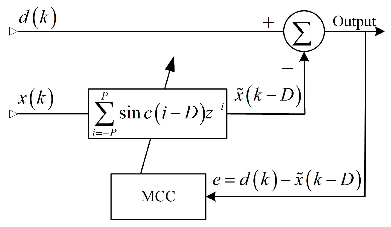
2.1. Maximum Correntropy Criterion

The correntropy, measuring the similarity between two arbitrary scalar random variables X and Y, is defined by:

$$V_{\sigma }\left(X,Y\right)=E\left[k_{\sigma }\left(X-Y\right)\right]$$

(7)

where $k_{\sigma }$ is a shift-invariant Mercer kernel with kernel size $\sigma$, and $E\left[·\right]$ is the mathematic expectation. Using the most popular Gaussian kernel $G_{\sigma }$ and substituting $E\left[·\right]$ by the most recent L samples estimator, the correntropy estimator becomes:

$$\begin{array}{ccc}\hfill {\widehat{V}}_{\sigma }\left(X-Y\right)& =& \frac{1}{L}\sum _{i=k-L+1}^k{G}_{\sigma }(x\left(i\right)-y\left(i\right))\hfill \\ & =& \frac{1}{L}\sum _{i=k-L+1}^k\frac{1}{\sqrt{2\pi }\sigma }exp\left(-\frac{{\left(x\left(i\right)-y\left(i\right)\right)}^2}{2{\sigma }^2}\right)\hfill \end{array}$$

(8)

In the adaptive filter, the correntropy estimator between the desired signal $d_i$ and the filter output $y_i$ is used as the cost function, then we get the cost function at k moment:

$$J\left(k\right)=\frac{1}{\sqrt{2\pi }\sigma L}\sum _{i=k-L+1}^{k}exp\left(-\frac{{\left(d\left(i\right)-y\left(i\right)\right)}^2}{2{\sigma }^2}\right)$$

(9)

The cost function $J\left(k\right)$ is maximized using the stochastic gradient and the filter coefficient vector $\mathbf{W}$ is updated online:

$$\mathbf{W}(k+1)=\mathbf{W}\left(k\right)+\mu \nabla J\left(k\right)$$

(10)

$J\left(k\right)$ is substituted in (9), then we obtain:

$$\mathbf{W}(k+1)=\mathbf{W}\left(k\right)+\frac{\mu }{\sqrt{2\pi }{\sigma }^{3}L}\sum _{i=k-L+1}^k\left[exp\left(\frac{-e{\left(i\right)}^2}{2{\sigma }^2}\right)e\left(i\right)\mathbf{x}\left(i\right)\right]$$

(11)

where $e\left(i\right)=d\left(i\right)-\mathbf{W}{\left(k\right)}^T\mathbf{x}\left(i\right)$ and $\mu$ is a positive scalar. As shown in (11), when the errors increase, the weighting term decreases exponentially, and shows robust in impulsive noise environments.

When MEE criterion is used to train the adaptive filter, the filter coefficient vector ${\mathbf{W}}_{\mathbf{MEE}}$ is updated online [21]:

$${\mathbf{W}}_{MEE}(k+1)={\mathbf{W}}_{MEE}\left(k\right)+\frac{\mu }{\sqrt{2\pi }{\sigma }^3{L}^2}\sum _{n=k-L+1}^k\sum _{i=k-L+1}^k\left[exp\left(\frac{-{\left(e\left(n\right)-e\left(i\right)\right)}^2}{2{\sigma }^2}\right)\left(e\left(n\right)-e\left(i\right)\right)\left(\mathbf{x}\left(n\right)-\mathbf{x}\left(i\right)\right)\right]$$

(12)

For the most recent L samples, the computational complexity of MCC algorithm is $O\left(L\right)$. The computation of entropy for L samples involves a double sum over all the samples and the computational complexity of MEE algorithm is $O\left(L^2\right)$ [22]. Therefore, the computational complexity of MEE algorithm is much higher than that of MCC algorithm and MEE algorithm is unsuitable for real-time implementation.

2.2. Explicit Time Delay Estimation

Suppose that the relationship between $d\left(k\right)$ and $x\left(k\right)$ is:

$$d\left(k\right)=Ax\left(k-D\right)$$

(13)

where A is the attenuation factor and D is the time delay between the primary channel and reference channel. As shown in Figure 2, the finite impulse response (FIR) filter coefficients are replaced by a truncated sinc function in ETDE algorithm, then $x\left(k-D\right)$ can be expressed as:

$$\tilde{x}\left(k-D\right)=\sum _{i=-P}^{P}x\left(k-i\right)sinc\left(i-D\right)$$

(14)

where, P should be set large enough to reduce the time delay modeling error and

$$sinc\left(u\right)=\frac{sin\left(\pi u\right)}{\pi u}$$

(15)

When maximum correntropy criterion is used in ETDE algorithm, the cost function becomes:

$$J_{ETDE}\left(D\right)=\frac{1}{L}\sum _{i=k-L+1}^k{G}_{\sigma }(d\left(i\right)-\tilde{x}\left(i-D\right))$$

(16)

Then, the time delay estimation value $D\left(k+1\right)$ at $(k+1)$th iteration can be obtained through:

$$D(k+1)=D\left(k\right)-\frac{\mu }{{\sigma }^2}{G}_{\sigma }\left(e\left(k\right)\right)e\left(k\right)\sum _{\mathrm{j}=-P}^{P}x\left(k-j\right)f\left(j-D\left(k\right)\right)$$

(17)

where $f\left(v\right)=\left(cos\right(\pi v)-sinc(v\left)\right)/v$.

2.3. Time Delay Compensation

When the reference inputs are used to reduce the noise, we need to know, not only the time-varying delays between primary input and reference inputs, but also which channel to be selected to collect the correlated noise. Because, if the reference noise is not correlated to the noise in the primary input, adaptive filter will not work and the SNR of output will decrease. Through time delay estimation, we can know the time-varying delay and relationship between primary input and reference inputs. For example, if the primary input and reference input 1 are correlated, the time delay estimation will converge to the steady state with a certain value and the noise in reference input 1 is chosen as reference noise. The proposed method works as shown in Figure 3.

• Time Delay Estimation

As shown in Figure 3, each reference input has an individual delay estimation module which estimates the time delay between primary input and reference input. The more correlated the noises are, the more accurate the estimated time delay is. If the SNR in the primary input is not very low, the communication signals cause a big error in time delay estimation. Therefore, the time delay estimation module may fail to converge in the communication process. In practical applications, the time delay should be corrected in the communication gap, based on the assumption that the noise source is the same during a communication process.

• Delay and Channel Control

The delay and channel control module is used to set the time delay in primary input and chose the reference input. The time delay values obtained from the delay estimation modules of reference inputs are compared in this module. The reference input selected as the reference noise is the input with more accurate time delay value, having a smaller variance. Then the time delay is compensated to make sure that the delay between primary input and reference input is almost half the time delay of the adaptive filter.

• Noise Cancellation

With time delay compensation, the adaptive filter can cover most significant part of the noise path’s impulse response with a limited number of coefficients [25]. In addition, the ANC algorithm can be only applied to the active regions where the communication signals appear [24]. As a result, the complexity of ANC algorithm is reduced and the performance is greatly improved.

3. FPGA Implementation

As shown in Figure 3, the proposed algorithm includes three modules: time delay estimation module, delay and channel control module, and noise cancellation module. As shown in Equation (17), there are (2P + 1) multiply-accumulate operations and one exponential operation for each sample to get the time delay estimation value. In order to obtain high time delay estimation accuracy, all the operations should be executed in one sampling period and the sampling period should be reduced [31]. Therefore, acceleration of computing is needed. FPGA is more suitable for multiple-instruction, single-data (MISD) applications when power and space considerations outweigh price [32]. In order to execute the proposed algorithm in real time, the proposed algorithm is implemented on FPGA. In this paper, the sampling frequency is 1 MHz and the ADC is 14 bit. Next, this system is described in detail.

Figure 4 shows the time delay estimation block diagram. For each channel, the noise signal $x\left(k\right)$ is stored in register stack and P is set to be 32. Through the multiply-accumulate (MAC) operation, the noise signal $x\left(k\right)$ is multiplied by sinc and $f\left(v\right)$ functions. To reduce the computational complexity, the sinc and $f\left(v\right)$ functions are stored in two lookup tables. The values of sinc and $f\left(v\right)$ functions are obtained from the lookup tables, based on the time delay estimation value $D\left(k\right)$ from previous iteration. Then the time delay estimation value is updated based on Equation (17).

After getting the time delay values of all channels, the values are processed by the delay control module, which is shown in Figure 5. In order to reduce the computational complexity, we use mean absolute error (MAE) of $D\left(k\right)$ rather than the variance to evaluate the correlation between the primary input and the reference inputs. Then the reference input with least MAE will be selected as the reference noise. We will also obtain the time delay value $D_{\mathrm{c}}\left(k\right)$ inserted in the primary input:

$$D_c\left(k\right)=E\left[D\left(k\right)\right]+\frac{L_W}{2}$$

(18)

where, $L_W$ is the length of coefficient vector $\mathbf{W}$.

Figure 6 shows the adaptive noise cancellation block diagram. The desired signal with the delay $D_C\left(k\right)$ is subtracted by the filter output, which is obtained through MAC operation. As we have known the time delay between the primary input and the reference input, we can shorten the filter length. In this paper, the length of filter coefficient is 4 and the filter coefficient vector is updated based on Equation (11).

The proposed algorithm is implemented with the Altera Stratix III EP3SE260F1152C2N FPGA.

Table 1. Hardware Resource Consumption.

Module	ALUTs	Block Memory (Kbits)	DSP Block
MCC-ETDE	16,478	2048	309
Control Module	867	0	0
ANC	1620	0	32
Total Utilization	18,969	2048	341
Utilization Rate	9%	14%	44%

ALUT (Adaptive Look-Up Table); DSP (Digital Signal Processing); ANC ( adaptive Noise Cancellation).

lists the hardware resource consumption. For this design, the resources of the Stratix III EP3SE260F1152C2N are quite sufficient. The highest resource utilization module is the MCC-ETDE module, which requires 9 times more resource than the ANC module. In this paper, the length of filter coefficient is 4. Therefore, the resource utilization of ANC module is equal to that of the MCC-ETDE module when the length of filter coefficient is 40. In the actual situation, the proposed algorithm can reduce the hardware resource consumption when the time delay is more than 40 samples.

4. Results and Discussion

4.1. Evaluation Methods

In this section, the performance of the proposed ANC-TDE algorithm is evaluated by simulation and experiment. Suppose that the communication signal is single-frequency sinusoidal signal and frequency is 10 kHz. The sampling frequency is 1 MHz and the sample data is 14 bit.

4.1.1. Simulation Method

To evaluate the performance of the proposed adaptive noise cancellation algorithm by simulation, the proposed algorithm is implemented on the experimental board. As shown in Figure 7, the experimental board includes one main board and one DA/AD data conversion card. The 14-bit D/A data conversion card is used to generate two signals. One signal is the communication signal which is mixed with S$\alpha$S noise. Another signal is the S$\alpha$S noise with variable time delay. Then, the two signals are processed by the proposed algorithm after 14-bit A/D conversion.

To evaluate the performance of the proposed algorithm against impulsive noise, the noise is presented as the $S\alpha S$ process when $\alpha$ = 1.5, $\beta$ = 0, where the location parameter $\delta$ is 0 and the dispersion $\gamma$ is 1. In the non-Gaussian noise environment, the mixed SNR is defined in [33]

$$SN{R}_m=10{log}_{10}\left(\frac{{\sigma }_s^2}{\gamma }\right)$$

(19)

where ${\sigma }_s^2$ is the variance of the signal and $\gamma$ is the dispersion of the impulsive noise. Firstly, the time delay estimation performance and noise cancellation performance are evaluated in different mixed SNR environments respectively. Secondly, the noise cancellation performance of proposed algorithm is evaluated when the time delay between the primary input and reference input is changing.

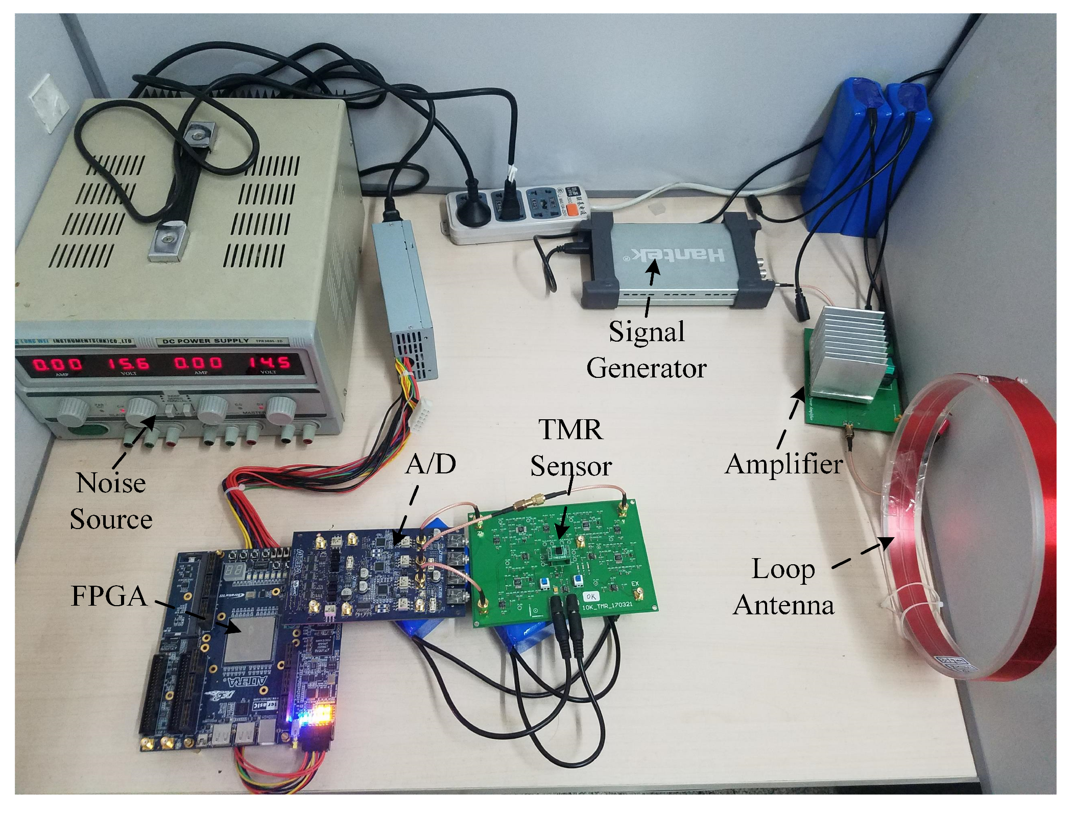
4.1.2. Experimental Method

In order to verify the practicability of the proposed algorithm, the adaptive noise cancellation system based is built on FPGA, which is shown in Figure 8. The sinusoidal signal with 10 kHz frequency is generated by the signal generator and is amplified by the amplifier. Then The signal is transmitted by the loop antenna, whose diameter is 20 cm. The transmitted magnetic signal is received by a three-channel tunneling magnetoresistance (TMR) sensor (TMR2305). The Y channel of TMR sensor is parallel to the axis of the loop antenna. The Y channel and X channel of TMR sensor are parallel to the horizontal plane. The Z channel of TMR sensor is vertical to the horizontal plane. The three channels are perpendicular to each other. After amplifiers, filters and 14-bit A/D converters, the received signals are processed by the FPGA. To generate the impulsive noise, a switched-mode power supply is used as the noise source. The comparison between original signal and filter output is made to show the noise cancellation performance of proposed algorithm.

4.2. Simulation Results

4.2.1. Time Delay Estimation Performance

Figure 9 shows the time delay estimation performance of MCC-ETDE algorithm when the primary input has no communication signal. Therefore, all the input signals are the correlated impulsive noises. The time delay between the primary input and reference input is 10 $T_s$. The Gaussian kernel size $\sigma$ is 0.5 and the positive scalar $\mu$ is 0.4. The MCC-ETDE algorithm can converge to the true time delay whin 1000 times of iterations (1 ms) and is suitable for real-time communication. When the pulses occur, the MCC-ETDE algorithm has bigger errors but will come back to the steady state very soon.

Figure 10 shows the time delay estimation performance of MCC-ETDE algorithm when the mixed SNR in the primary input is −23 dB. When MCC-ETDE algorithm estimates the time delay between the noise of the primary input and that of the reference input, the communication signal becomes an interference signal. As shown in Figure 10, the communication signal has no major impact on the convergence speed but causes big steady-state error, which affects the noise cancellation performance.

Figure 11 shows the time delay estimation variance of MCC-ETDE algorithm at different mixed SNR levels. The time delay estimation variance of MCC-ETDE algorithm increases when the mixed SNR increases. Therefore, in the communication process, the MCC-ETDE algorithm may not converge to the steady state because of the communication signal. We should obtain the time delay and relationship between the primary input and reference input among communication gap.

4.2.2. Noise Cancellation Performance

In this paper, the noises in the primary input and the reference input are in the same amplitude and the time delay is set to be 2 $T_s$. The length of filter coefficient vector is set to be 4. In the MCC algorithm, the Gaussian kernel size $\sigma$ is 2 and the positive scalar $\mu$ is 0.5. In the LMS algorithm, the positive scalar $\mu$ is 0.0002. Figure 12 shows the square error of the filter coefficient vector of LMS algorithm and MCC algorithm when mixed SNR in the primary input is −23 dB. The MCC algorithm has faster convergence speed and smaller square error than the LMS algorithm in the impulsive noise. Figure 13 shows the square error of signal of LMS algorithm and MCC algorithm when mixed SNR in the primary input is −23 dB. In the steady state, the LMS algorithm has much bigger square error than the MCC algorithm when the pulses occur.

To compare the noise cancellation performance between LMS algorithm and MCC algorithm at different mixed SNR levels, the noise is kept at the same magnitude and the magnitude of communication signal is changed. During this process, the parameters of LMS algorithm and MCC algorithm are not changed. Figure 14 shows the MSE (Mean Squared Error) of filter output at different mixed SNR levels. The mixed SNR has different effects on LMS algorithm and MCC algorithm. As the mixed SNR increases, the MSE of LMS algorithm slightly decreases. However, the MSE of MCC algorithm increases when the mixed SNR increases, because the increased amplitude of communication signal has a greater impact on the Gaussian kernel function. To obtain smaller MSE, the Gaussian kernel size should be changed. Nevertheless, the MSE of MCC algorithm is much smaller than that of the LMS algorithm.

4.2.3. Time Delay Compensation Result

The traditional noise cancellation algorithm can only be applied in some certain circumstances where the primary input lags behind the reference inputs. In this paper, the simulation is carried out in the circumstance where the reference input lags behind the primary input. Figure 15 shows the time delay control performance of proposed algorithm when mixed SNR in the primary input is −23 dB. In the interval $\left[0,1500\right)$ and $\left[5000,6500\right)$, there is only noise in the primary input. In the interval $\left[1500,5000\right)$ and $\left[6500,10000\right)$, the communication signal is added to the primary input. In the interval $\left[1500,5000\right)$, the time delay is set to be 3 $T_s$. Then, the time delay is set to be 4 $T_s$. When there is only the noise in the primary input, the MCC-ETDE algorithm can estimate the time delay without error. When the communication signal is added to the primary input, the time delay estimation values will have bigger variance. When the MAE of time delay estimate values is bigger than the threshold, the time delay control module will select the previous value as the time delay. The threshold is set based on the actual situation. As shown in Figure 15, the time delay control (TDC) values can converge to the true time delay values.

Figure 16 shows the adaptive noise cancellation performance of proposed algorithm when mixed SNR in the primary input is −23 dB. As shown in Figure 16b, before the time delay estimation module obtains the time delay, the adaptive noise cancellation module cannot improve the SNR in the primary input. After obtaining the true time delay, the adaptive noise cancellation module achieves very good noise cancellation performance with the time delay compensated in the primary input. In addition, the proposed algorithm can track the changes of time delay with a fast convergence speed. When the time delay changes, the proposed algorithm still obtains good noise cancellation performance with a period of time to compensate the varied time delay. In Figure 16c, the noise cancellation performance without time delay compensation after 5000 samples is shown. Without time delay compensation, the adaptive noise cancellation module cannot remove the noise from the signal.

4.3. Experimental Results

Figure 17 shows the signals that are received by the TMR sensor. All the three channels receive the noise that is generated by the power supply. The Y channel has the maximum-amplitude transmitted signal, and Z channel has the minimum-amplitude transmitted signal. Therefore, the Y channel is selected as the primary input, and the Z channel is selected as the noise reference. Figure 18 shows the adaptive noise cancellation performance of the proposed algorithm. After processed by the FPGA, the impulsive noise in the received signal is cancelled and the proposed algorithm can increase the SNR about 6 dB in this experiment.

5. Conclusions

In order to improve the SNR for low frequency electromagnetic TTE communication, the ANC-TDE algorithm based on MCC is proposed and implemented on FPGA in this paper. As shown in the simulation and experiment results, the proposed algorithm can adaptively compensate the varied time delay between the primary input and the reference input. With the time delay compensated, the proposed algorithm can reduce the complexity of the ANC filter and improve the noise cancellation performance in the impulsive noise environment.

In the future work, we plan to conduct noise cancellation experiments in the real TTE environments and optimize parameters of proposed algorithm according to noise characteristics in different applications.

References

1. Ma, J.; Zhang, X.; Huang, Q. Near-field magnetic induction communication device for underground wireless communication networks. Sci. China Inf. Sci. 2014, 57, 1–11. [Google Scholar] [CrossRef]
2. Ma, J.; Zhang, X.; Huang, Q.; Cheng, L.; Lu, M. Experimental Study on the Impact of Soil Conductivity on Underground Magneto-Inductive Channel. IEEE Antennas Wirel. Propag. Lett. 2015, 14, 1782–1785. [Google Scholar] [CrossRef]
3. Goswami, J.C.; Hoefel, A.E.; Schwetlick, H. On subsurface wireless data acquisition system. IEEE Trans. Geosci. Remote Sens. 2005, 43, 2332–2339. [Google Scholar] [CrossRef]
4. Sheinker, A.; Ginzburg, B.; Salomonski, N.; Frumkis, L.; Kaplan, B.Z. Localization in 3-D using beacons of low frequency magnetic field. IEEE Trans. Instrum. Meas. 2013, 62, 3194–3201. [Google Scholar] [CrossRef]
5. Devaney, A.J. Time reversal imaging of obscured targets from multistatic data. IEEE Trans. Antennas Propag. 2005, 53, 1600–1610. [Google Scholar] [CrossRef]
6. Dalgaard, E.; Auken, E.; Larsen, J.J. Adaptive noise cancelling of multichannel magnetic resonance sounding signals. Geophys. J. Int. 2012, 191, 88–100. [Google Scholar] [CrossRef]
7. Forooshani, A.E.; Bashir, S.; Michelson, D.G.; Noghanian, S. A survey of wireless communications and propagation modeling in underground mines. IEEE Commun. Surv. Tutor. 2013, 15, 1524–1545. [Google Scholar] [CrossRef]
8. Compston, A.J.; Fluhler, J.D.; Schantz, H.G. A fundamental limit on antenna gain for electrically small antennas. In Proceedings of the IEEE Sarnoff Symposium, Princeton, NJ, USA, 28–30 April 2008; pp. 1–5. [Google Scholar]
9. Schlegel, C.; Mallay, M.; Touesnard, C. Atmospheric Magnetic Noise Measurements in Urban Areas. IEEE Magn. Lett. 2014, 5, 1–4. [Google Scholar] [CrossRef]
10. Yan, L.; Waynert, J.; Sunderman, C.; Damiano, N. Statistical analysis and modeling of VLF/ELF noise in coal mines for through-the-earth wireless communications. In Proceedings of the 2014 IEEE Industry Applications Society Annual Meeting, Vancouver, BC, Canada, 5–9 October 2014; pp. 1–5. [Google Scholar]
11. Middleton, D. Non-Gaussian noise models in signal processing for telecommunications: New methods an results for class A and class B noise models. IEEE Trans. Inf. Theory 1999, 45, 1129–1149. [Google Scholar] [CrossRef]
12. Ciuonzo, D.; Romano, G.; Solimene, R. Performance analysis of time-reversal MUSIC. IEEE Trans. Signal Process. 2015, 63, 2650–2662. [Google Scholar] [CrossRef]
13. Ciuonzo, D.; Salvoi-Rossi, P. Noncolocated time-reversal MUSIC: High-SNR distribution of null spectrum. IEEE Signal Process. Lett. 2017, 24, 397–401. [Google Scholar] [CrossRef]
14. Raab, F.H.; Joughin, I.R. Signal processing for through-the-earth radio communication. IEEE Trans. Commun. 1995, 43, 2995–3003. [Google Scholar] [CrossRef]
15. Quinquis, A.; Rossignol, S. Noise reduction, with a noise reference, of underwater magnetic signals. Digit. Signal Process. 1996, 6, 240–248. [Google Scholar] [CrossRef]
16. Mitchell, D.; Robertson, J. Reference antenna techniques for canceling radio frequency interference due to moving sources. Radio Sci. 2005, 40, 1–9. [Google Scholar] [CrossRef]
17. Haykin, S.S. Adaptive Filter Theory; Pearson Education India: Noida, India, 2008. [Google Scholar]
18. Walach, E.; Widrow, B. The least mean fourth (LMF) adaptive algorithm and its family. IEEE Trans. Inf. Theory 1984, 30, 275–283. [Google Scholar] [CrossRef]
19. Pei, S.C.; Tseng, C.C. Least mean p-power error criterion for adaptive FIR filter. IEEE J. Sel. Areas Commun. 1994, 12, 1540–1547. [Google Scholar]
20. Wang, R.; Chen, B.; Zheng, N.; Principe, J.C. A variable step-size adaptive algorithm under maximum correntropy criterion. In Proceedings of the 2015 International Joint Conference on Neural Networks (IJCNN), Killarney, Ireland, 12–17 July 2015; pp. 1–5. [Google Scholar]
21. Principe, J.C. Information Theoretic Learning: Renyi’s Entropy and Kernel Perspectives; Springer Science & Business Media: Berlin/Heidelberg, Germany, 2010. [Google Scholar]
22. Singh, A.; Principe, J.C. Using correntropy as a cost function in linear adaptive filters. In Proceedings of the International Joint Conference on Neural Networks, Atlanta, GA, USA, 14–19 June 2009; pp. 2950–2955. [Google Scholar]
23. Widrow, B.; Stearns, S.D. Adaptive Signal Processing; Prentice-Hall, Inc.: Englewood Cliffs, NJ, USA, 1985; 491p. [Google Scholar]
24. Lu, Y.; Fowler, R.; Tian, W.; Thompson, L. Enhancing echo cancellation via estimation of delay. IEEE Trans. Signal Process. 2005, 53, 4159–4168. [Google Scholar]
25. Sugiyama, A.; Miyahara, R.; Kato, M. An adaptive noise canceller with adaptive delay compensation for a distant noise source. In Proceedings of the 2011 IEEE International Conference on Acoustics, Speech and Signal Processing (ICASSP), Prague, Czech Republic, 22–27 May 2011; pp. 265–268. [Google Scholar]
26. Wang, P.; Zhang, X.; Sun, G.; Xu, L.; Xu, J. Adaptive time delay estimation algorithm for indoor near-field electromagnetic ranging. Int. J. Commun. Syst. 2016. [Google Scholar] [CrossRef]
27. Padilla, P.; Górriz, J.M.; Ramírez, J.; Salas-Gonzalez, D.; Illán, I. Intensity normalization in the analysis of functional DaTSCAN SPECT images: The α-stable distribution-based normalization method vs other approaches. Neurocomputing 2015, 150, 4–15. [Google Scholar] [CrossRef]
28. Laguna-Sanchez, G.; Lopez-Guerrero, M. On the use of alpha-stable distributions in noise modeling for PLC. IEEE Trans. Power Deliv. 2015, 30, 1863–1870. [Google Scholar] [CrossRef]
29. Fiche, A.; Cexus, J.C.; Martin, A.; Khenchaf, A. Features modeling with an α-stable distribution: Application to pattern recognition based on continuous belief functions. Inf. Fusion 2013, 14, 504–520. [Google Scholar] [CrossRef] [Green Version]
30. Yue, B.; Peng, Z. A validation study of α-stable distribution characteristic for seismic data. Signal Process. 2015, 106, 1–9. [Google Scholar] [CrossRef]
31. Dooley, S.R.; Nandi, A.K. Adaptive subsample time delay estimation using Lagrange interpolators. IEEE Signal Process. Lett. 1999, 6, 65–67. [Google Scholar] [CrossRef]
32. Sriram, V.; Tsoi, K.; Luk, W.; Cox, D. Design-space exploration of biologically-inspired visual object recognition algorithms using CPUs, GPUs, and FPGAs. Many-Core Reconfig. Supercomput. 2010. Available online: https://pdfs.semanticscholar.org/2610/9131cdb40d6928b806afef6a1b3b44088ca1.pdf (accessed on 20 April 2016).
33. Ma, X.; Nikias, C.L. Joint estimation of time delay and frequency delay in impulsive noise using fractional lower order statistics. IEEE Trans. Signal Process. 1996, 44, 2669–2687. [Google Scholar]
Figure 1. Adaptive noise cancellation with correlated noise at the primary and reference input.
Applsci 08 00734 g001
Figure 2. Explicit time delay estimation based on MCC (Maximum Correntropy Criterion).
Applsci 08 00734 g002
Figure 3. Adaptive noise cancellation based on time delay estimation.
Applsci 08 00734 g003
Figure 4. Time delay estimation block diagram.
Applsci 08 00734 g004
Figure 5. Delay control block diagram.
Applsci 08 00734 g005
Figure 6. Adaptive noise cancellation block diagram.
Applsci 08 00734 g006
Figure 7. Experimental board.
Applsci 08 00734 g007
Figure 8. Adaptive noise cancellation system.
Applsci 08 00734 g008
Figure 9. Time delay estimation performance without communication signal.
Applsci 08 00734 g009
Figure 10. Time delay estimation performance when mixed SNR (Signal-to-Noise Ratio) in the primary input is −23 dB.
Applsci 08 00734 g010
Figure 11. Time delay estimation variance at different mixed SNR levels.
Applsci 08 00734 g011
Figure 12. Square error of filter coefficient vector when mixed SNR in the primary input is −23 dB.
Applsci 08 00734 g012
Figure 13. Square error of signal when mixed SNR in the primary input is −23 dB.
Applsci 08 00734 g013
Figure 14. MSE of filter output at different mixed SNR levels.
Applsci 08 00734 g014
Figure 15. Time delay control performance when mixed SNR in the primary input is −23 dB.
Applsci 08 00734 g015
Figure 16. Adaptive noise cancellation performance when mixed SNR in the primary input is −23 dB: (a) original signal; (b) filter output with time delay estimation; (c) filter output without time delay estimation.
Applsci 08 00734 g016
Figure 17. The signals received by TMR (Tunneling MagnetoResistance) sensor.
Applsci 08 00734 g017
Figure 18. Adaptive noise cancellation performance.
Applsci 08 00734 g018